

Laminar Boundary Layer over a Serrated Backward-Facing Step

 , , , and
Abstract
1. Introduction
2. Methodology
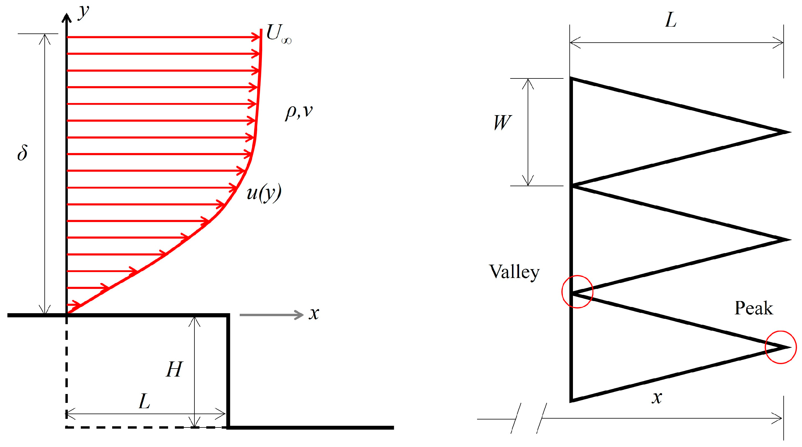
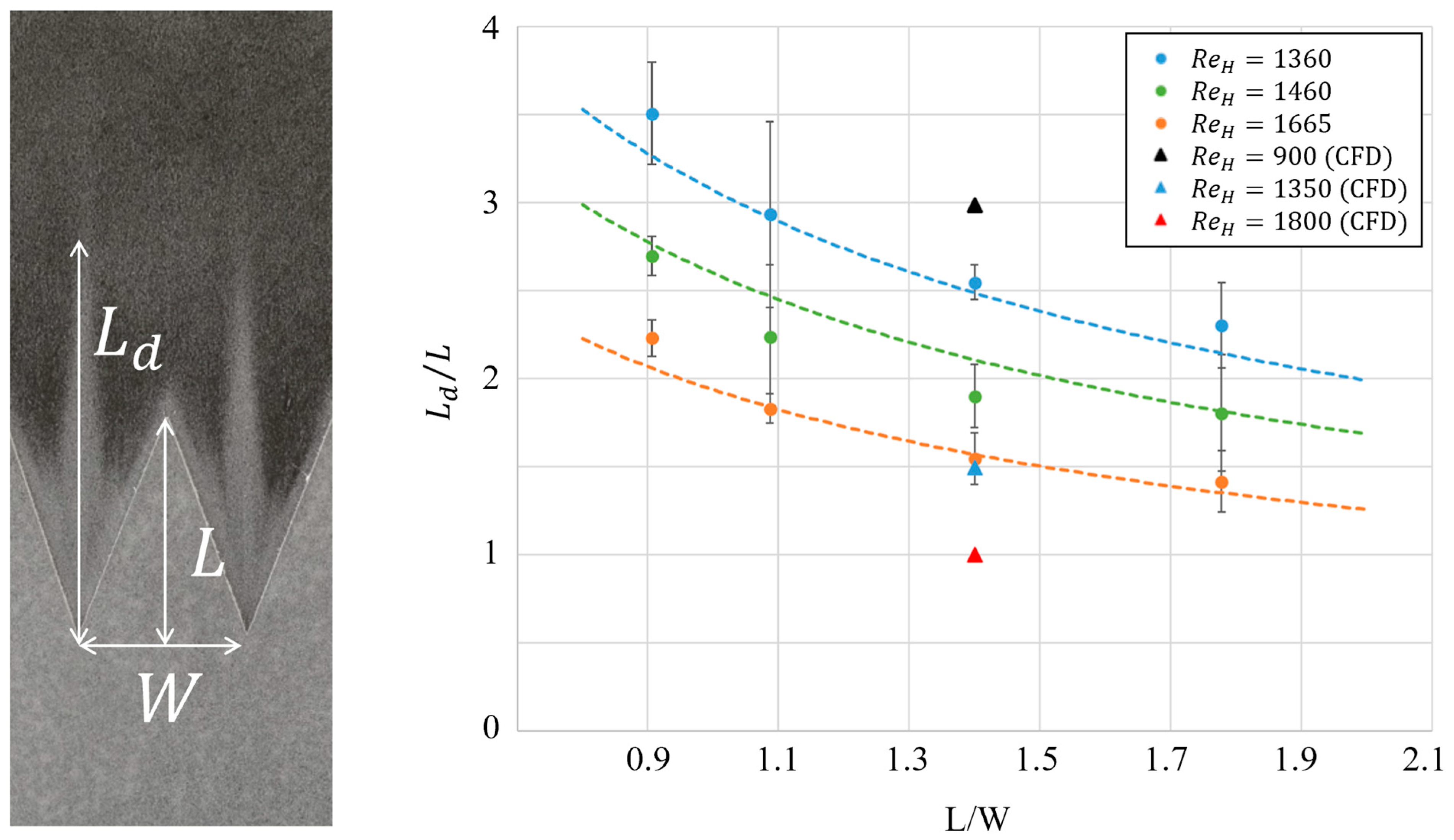
2.1. Scaling Law
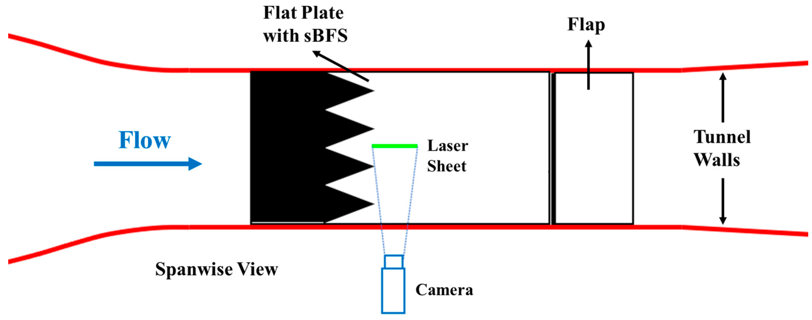
2.2. Experimental Methods
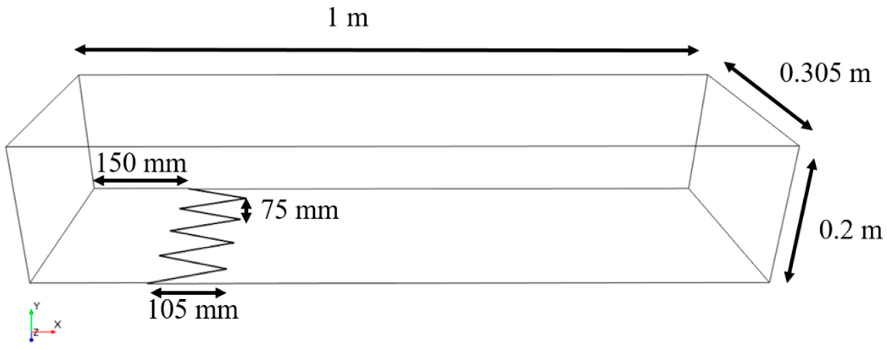
2.3. Computational Methods
3. Results
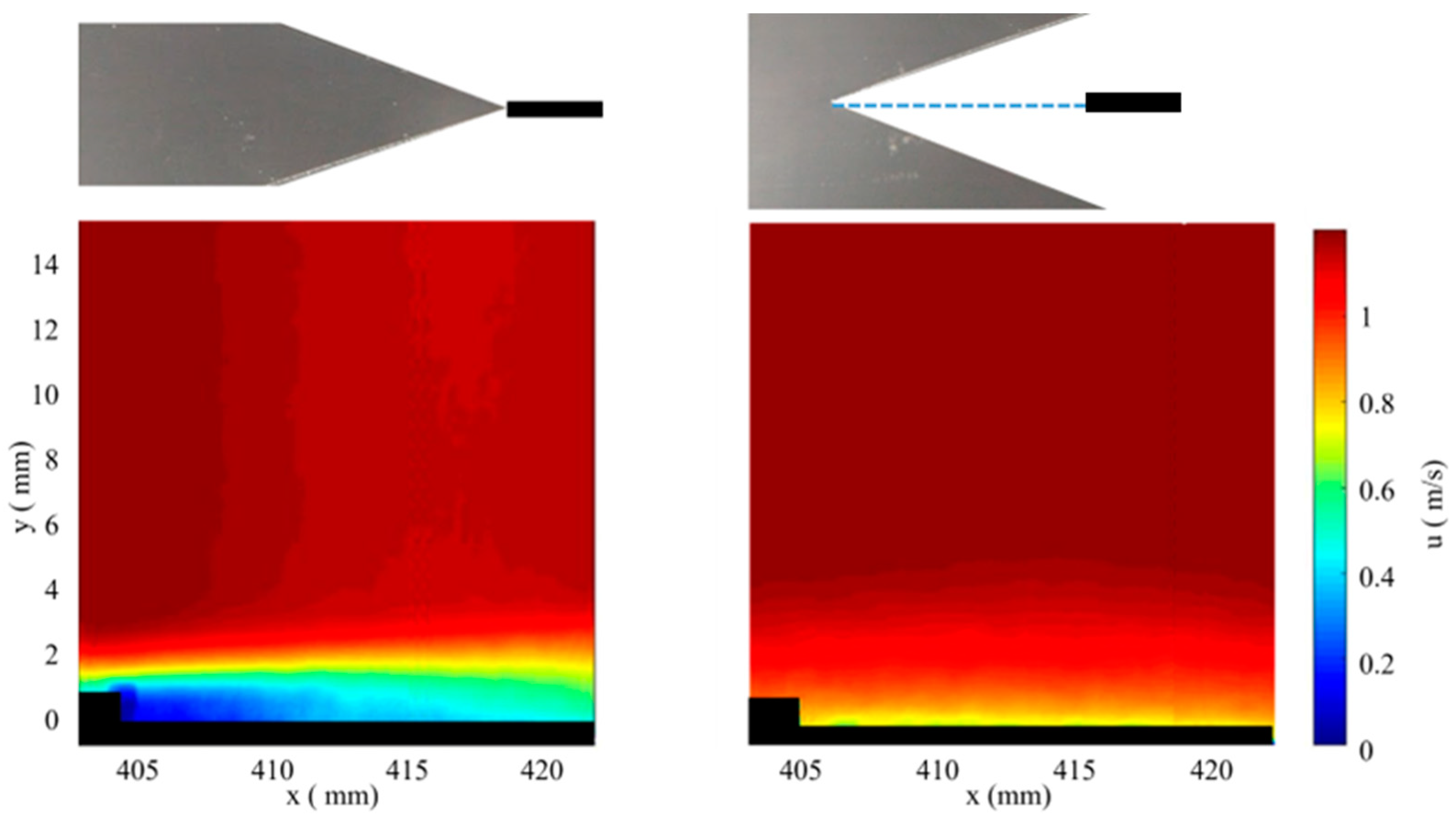
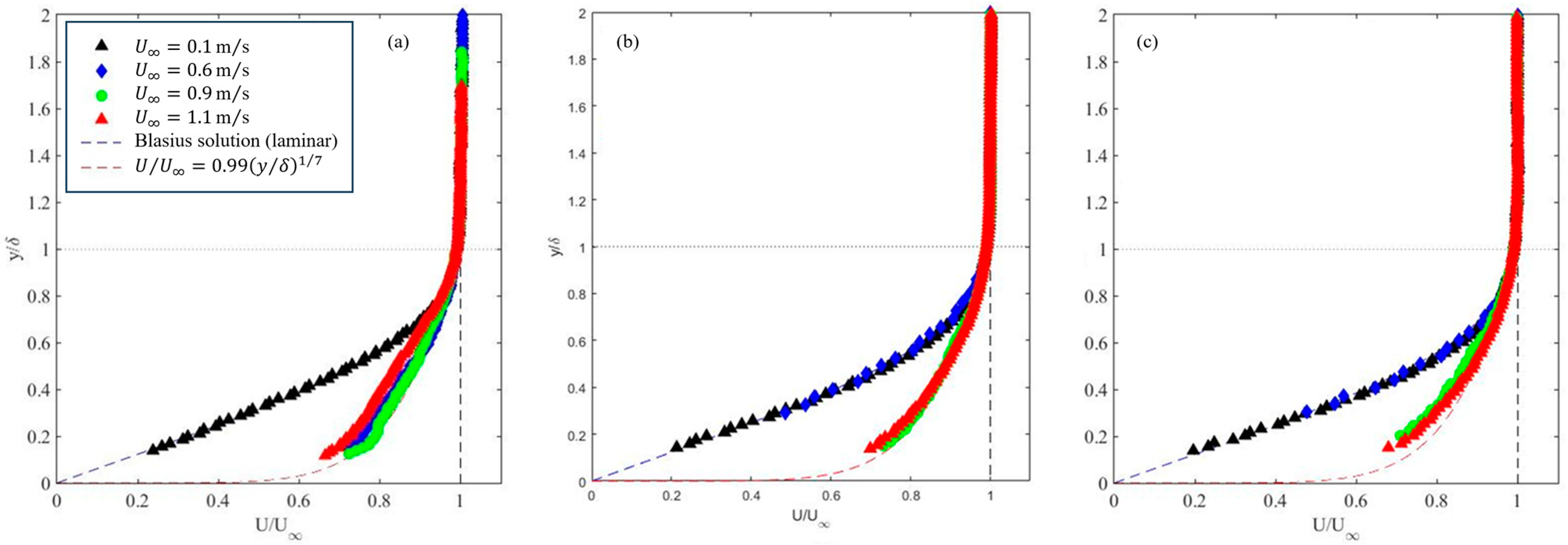
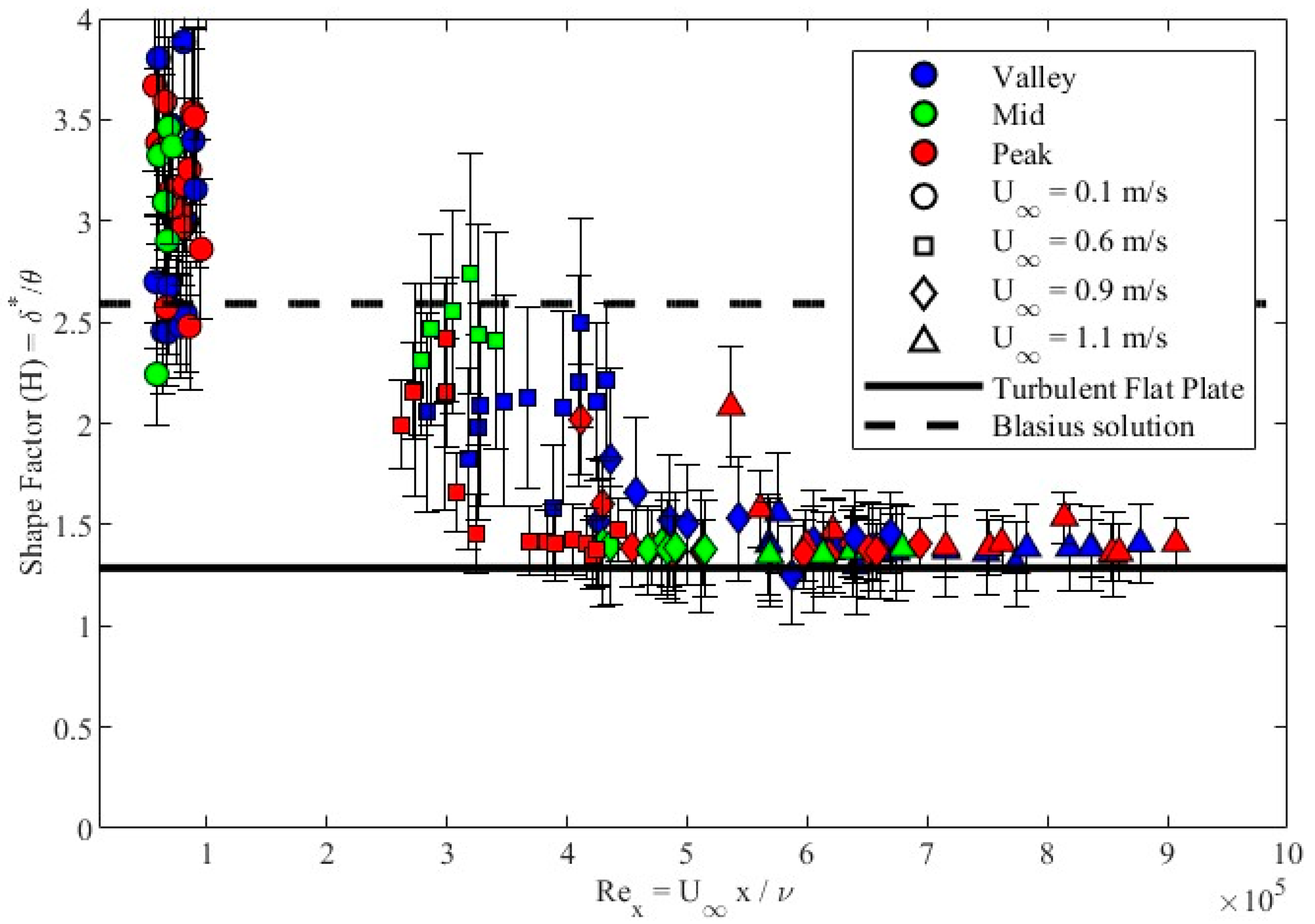
3.1. Experimental Results
3.1.1. Flat Plate
3.1.2. sBFS Model
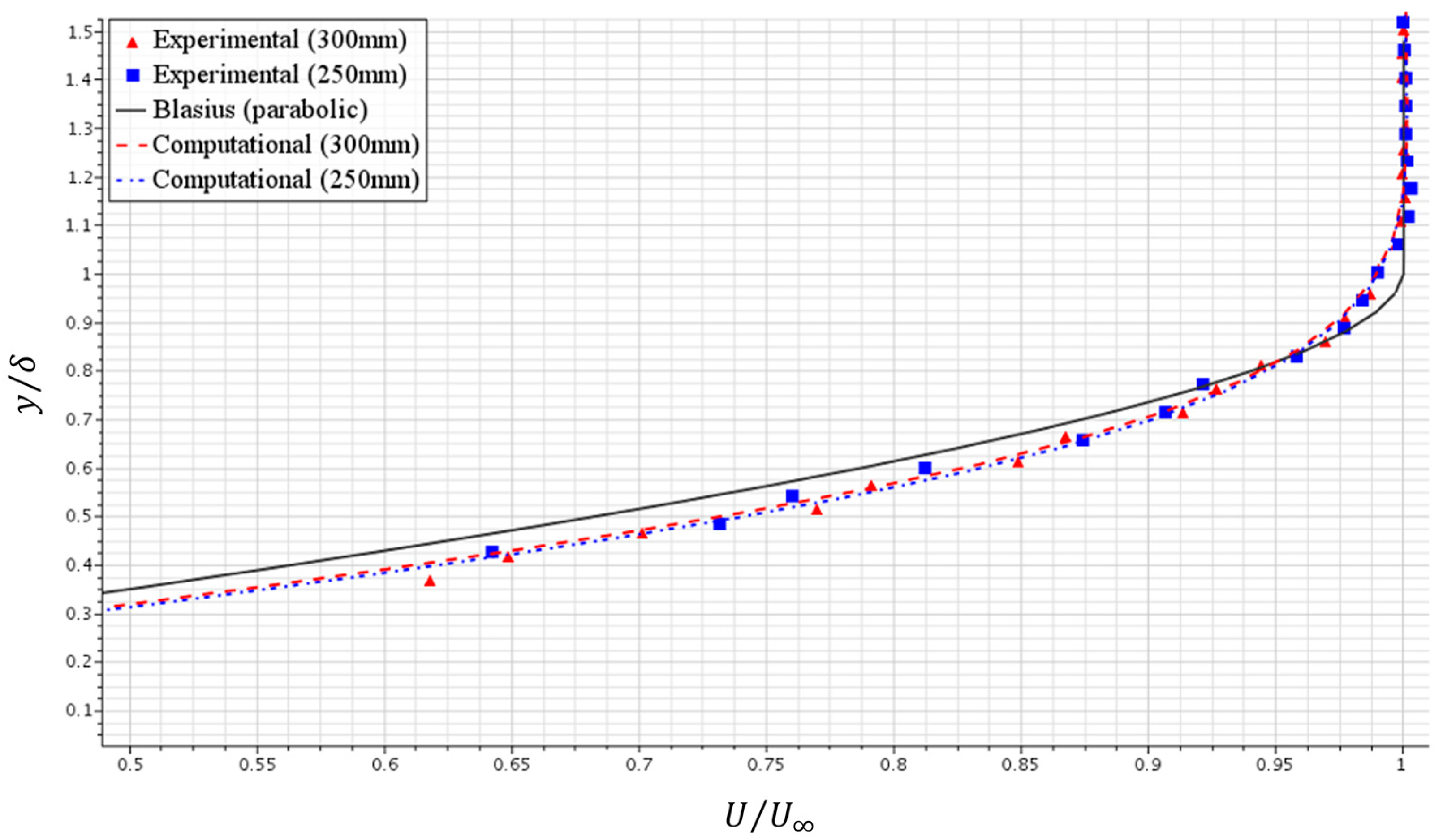
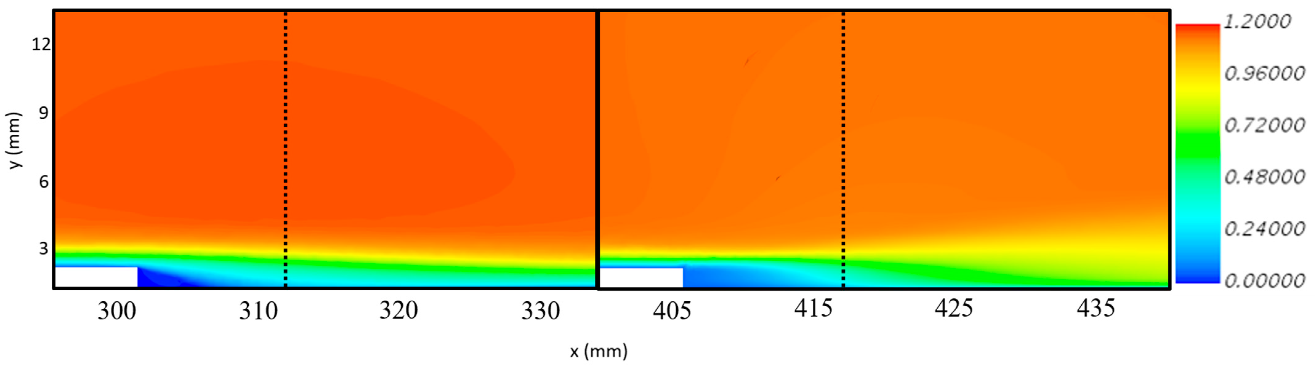
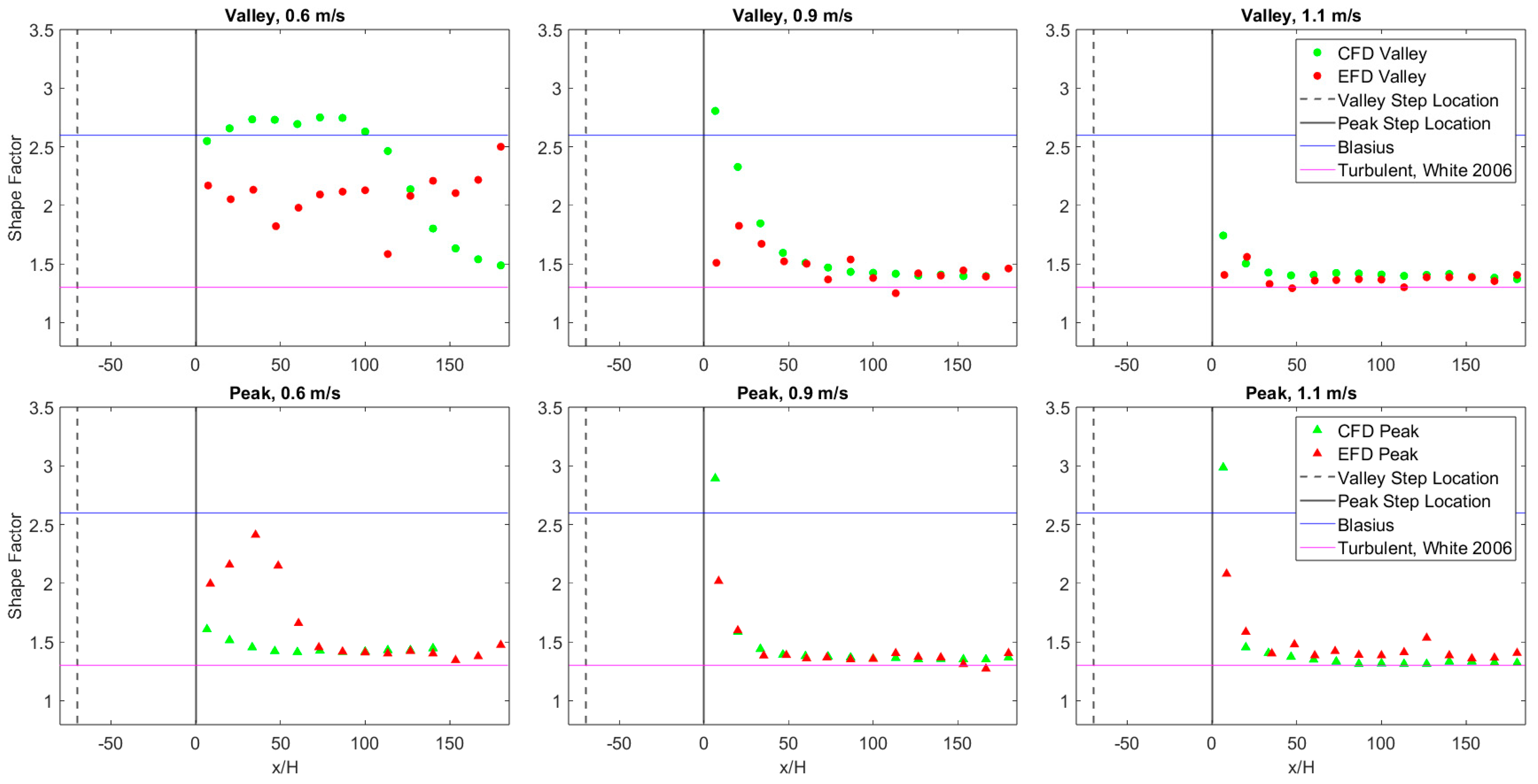
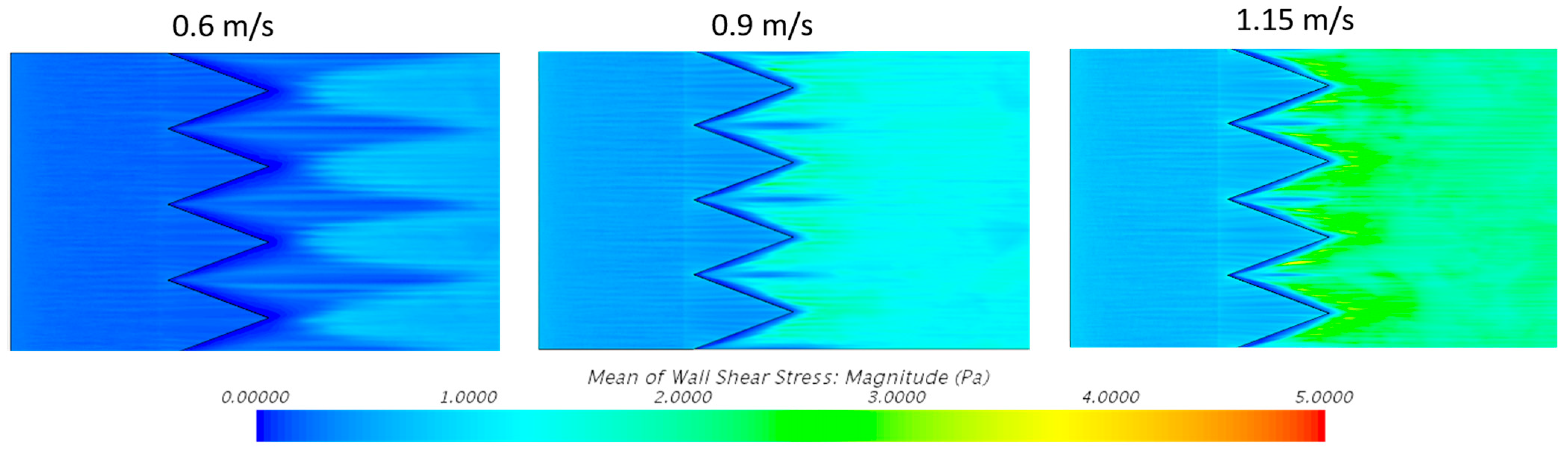
3.2. Computational Results
3.2.1. Flat Plate
3.2.2. Flat Plate with sBFS
4. Discussion
4.1. Extended sBFS CFD Analysis
4.2. Flight Test Comparison
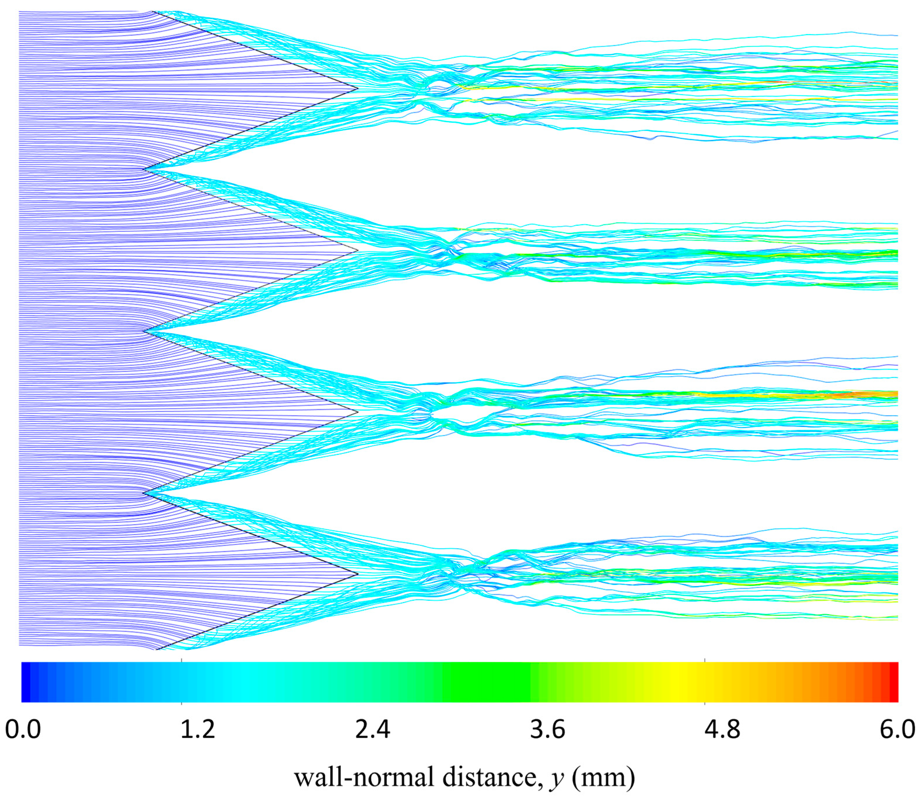
4.3. Near-Wall Flow Pattern
5. Conclusions
Author Contributions
Funding
Data Availability Statement
Acknowledgments
Conflicts of Interest
References
- Eaton, J.K.; Johnston, J.P. A review of research on subsonic turbulent flow reattachment. AIAA J. 1981, 19, 1093–1100. [Google Scholar] [CrossRef]
- Goldstein, R.J.; Eriksen, V.L.; Olson, R.M.; Eckert, E.R.G. Laminar separation, reattachment, and transition of the flow over a downstream-facing step. J. Fluids Eng. 1970, 92, 732–739. [Google Scholar] [CrossRef]
- Chang, P.K. Separation of Flow; Pergamon Press: Oxford, UK, 1970. [Google Scholar]
- Chen, L.; Asai, K.; Nonomura, T.; Xi, G.; Liu, T. A review of Backward-Facing Step (BFS) flow mechanisms, heat transfer and control. Therm. Sci. Eng. Prog. 2018, 6, 194–216. [Google Scholar] [CrossRef]
- Bolgar, I.; Scharnowski, S.; Kahler, C.J. Passive Flow Control for Reduced Load Dynamics Aft of a Backward-Facing Step. AIAA J. 2019, 57, 120–131. [Google Scholar] [CrossRef]
- Armaly, B.F.; Durst, F.; Pereira, J.C.F.; Schönung, B. Experimental and theoretical investigation of backward-facing step flow. J. Fluid. Mech. 1983, 127, 473–496. [Google Scholar] [CrossRef]
- Steinthorsson, E.; Liou, M.-S.; Povinelli, L.A.; Arnone, A. Numerical simulation of three-dimensional laminar flow over a backward facing step; Flow near side walls. In Proceedings of the ASME Fluids Engineering Division Summer Meeting, ICOMP-93-21, Washington, DC, USA, 20–24 June 1993. [Google Scholar]
- Major, D.; Palacios, J.; Maughmer, M.; Schmitz, S. A numerical model for the analysis of leading-edge protection tapes for wind turbine blades. J. Phys. Conf. Ser. 2020, 1452, 012058. [Google Scholar] [CrossRef]
- Major, D.; Palacios, J.; Maughmer, M.; Schmitz, S. Aerodynamics of leading-edge protection tapes for wind turbine blades. Wind. Eng. 2021, 45, 1296–1316. [Google Scholar] [CrossRef]
- Agrim, S.; Sapre, C.A.; Selig, M.S. Effects of leading-edge protection tape on wind turbine blade performance. Wind. Eng. 2012, 36, 525–534. [Google Scholar]
- Gerla, M.; Kleinrock, L. Flow control: A comparative survey. IEEE Trans. Commun. 1980, 28, 553–574. [Google Scholar] [CrossRef]
- Kostas, J.; Soria, J.; Chong, M. Particle image velocimetry measurements of a backward-facing step flow. Exp. Fluids 2002, 33, 838–853. [Google Scholar] [CrossRef]
- Storms, B.L.; Jang, C.S. Lift enhancement of an airfoil using a Gurney flap and vortex generators. J. Aircr. 1994, 31, 542–547. [Google Scholar] [CrossRef]
- Yao, C.; Lin, J.; Allen, B. Flowfield measurement of device-induced embedded streamwise vortex on a flat plate. In Proceedings of the 1st Flow Con-trol Conference, St. Louis, MO, USA, 24–26 June 2002. [Google Scholar]
- Fransson, J.H.; Talamelli, A.; Brandt, L.; Cossu, C. Delaying transition to turbulence by a passive mechanism. Phys. Rev. Lett. 2006, 96, 064501. [Google Scholar] [CrossRef] [PubMed]
- Shahinfar, S.; Sattarzadeh, S.S.; Fransson, J.H.; Talamelli, A. Revival of classical vortex generators now for transition delay. Phys. Rev. Lett. 2012, 109, 074501. [Google Scholar] [CrossRef] [PubMed]
- Siconolfi, L.; Camarri, S.; Fransson, J.H. Boundary layer stabilization using free-stream vortices. J. Fluid. Mech. 2015, 764, R2. [Google Scholar] [CrossRef]
- Babinsky, H.; Li, Y.; Ford, C.W.P. Microramp control of supersonic oblique shock-wave/boundary-layer interactions. AIAA J. 2009, 47, 668–675. [Google Scholar] [CrossRef]
- Chu, H.B.; Zhang, B.Q.; Chen, Y.C. Controlling flow separation of high lift transport aircraft with micro vortex generators. J. Northwestern Polytech. Univ. 2011, 29, 799–805. [Google Scholar]
- Paruchuri, C.; Joseph, P.; Ayton, L.J. On the superior performance of leading edge slits over serrations for the reduction of aerofoil interaction noise. In Proceedings of the 2018 AIAA/CEAS Aeroacoustics Conference, Atlanta, GA, USA, 25–29 June 2018; p. 3121. [Google Scholar]
- Yagiz, B.; Kandil, O.; Pehlivanoglu, Y.V. Drag minimization using active and passive flow control techniques. Aerosp. Sci. Technol. 2012, 17, 21–31. [Google Scholar] [CrossRef]
- Kibble, G.A. Experimental and Computational Investigation of the Conformal Vortex Generator. Master’s Thesis, Oklahoma State University, Stillwater, OK, USA, 2017. [Google Scholar]
- Mishnaevsky, L., Jr.; Hasager, C.B.; Bak, C.; Tilg, A.M.; Bech, J.I.; Rad, S.D.; Fæster, S. Leading edge erosion of wind turbine blades: Understanding, prevention and protection. Renew. Energy 2021, 169, 953–969. [Google Scholar] [CrossRef]
- Scholbrock, A. Power Performance Results UsingWind Turbine Blade Enhancing Devices Developed by Edge Aerodynamix; Technical Report; National Renewable Energy Laboratory: Golden, CO, USA, 2017. [Google Scholar]
- KC, R.J.; Wilson, T.C.; Alexander, A.S.; Jacob, J.D.; Lucido, N.A.; Elbing, B.R. Evaluation of a Serrated Edge to Mitigate the Adverse Effects of a Backward-Facing Step on an Airfoil. Inventions 2023, 8, 160. [Google Scholar] [CrossRef]
- Lucido, N.A.; KC, R.; Wilson, T.C.; Jacob, J.D.; Alexander, A.S.; Elbing, B.R.; Ireland, P.; Black, J.A. Laminar Boundary Layer Scaling Over a Conformal Vortex Generator. In Proceedings of the AIAA Scitech 2019 Forum, San Diego, CA, USA, 7–11 January 2019. [Google Scholar] [CrossRef]
- Wilson, T.C.; KC, R.; Lucido, N.A.; Elbing, B.R.; Alexander, A.S.; Jacob, J.D.; Ireland, P.; Black, J.A. Computational Investigation of the Conformal Vortex Generator. In Proceedings of the AIAA Scitech 2019 Forum, San Diego, CA, USA, 7–11 January 2019. [Google Scholar] [CrossRef]
- Drela, M. XFOIL Subsonic Airfoil Development System. 2018. Available online: http://web.mit.edu/drela/Public/web/xfoil/ (accessed on 31 May 2024).
- Patel, V. Calibration of the Preston tube and limitations on its use in pressure gradients. J. Fluid. Mech. 1965, 23, 185–208. [Google Scholar] [CrossRef]
- Schlichting, H.; Gersten, K. Boundary-Layer Theory, 9th ed.; Springer: Berlin, Germany, 2018. [Google Scholar]
- Wieneke, B. PIV uncertainty quantification from correlation statistics. Meas. Sci. Technol. 2015, 26, 074002. [Google Scholar] [CrossRef]
- Shams, A.; Roelofs, F.; Komen, E.M.J.; Baglietto, E. Quasi-direct numerical simulation of a pebble bed configuration, Part I: Flow (velocity) field analysis. Nucl. Eng. Des. 2013, 263, 473–489. [Google Scholar] [CrossRef]
- Shams, A.; Roelofs, F.; Komen, E.M.J.; Baglietto, E. Quasi-direct numerical simulation of a pebble bed configuration, Part-II: Temperature field analysis. Nucl. Eng. Des. 2013, 263, 490–499. [Google Scholar] [CrossRef]
- Kundu, P.K.; Cohen, I.M.; Dowling, D.R. Fluid Mechanics, 6th ed.; Academic Press: Cambridge, MA, USA, 2016. [Google Scholar]
- White, F.M.; Corfield, I. Viscous Fluid Flow; McGraw-Hill: New York, NY, USA, 2006; Volume 3. [Google Scholar]


| Parameter | Flight Scale Value |
|---|---|
| Parameter | Water Tunnel Scale | Units |
|---|---|---|
| mm | ||
| mm | ||
| mm | ||
| mm | ||
| Volume | m | |
| 2–2.5 | mm | |
| Δy | <y+ | |
| Δx | 30 y+ | |
| Δz | 30 y+ | |
| s | ||
| Cell count | 65 | million cells |
| Mesh | (m) | (mm) | ||
|---|---|---|---|---|
Disclaimer/Publisher’s Note: The statements, opinions and data contained in all publications are solely those of the individual author(s) and contributor(s) and not of MDPI and/or the editor(s). MDPI and/or the editor(s) disclaim responsibility for any injury to people or property resulting from any ideas, methods, instructions or products referred to in the content. |
© 2024 by the authors. Licensee MDPI, Basel, Switzerland. This article is an open access article distributed under the terms and conditions of the Creative Commons Attribution (CC BY) license (https://creativecommons.org/licenses/by/4.0/).
Share and Cite
KC, R.J.; Wilson, T.C.; Lucido, N.A.; Alexander, A.S.; Jacob, J.D.; Elbing, B.R. Laminar Boundary Layer over a Serrated Backward-Facing Step. Fluids 2024, 9, 135. https://doi.org/10.3390/fluids9060135
KC RJ, Wilson TC, Lucido NA, Alexander AS, Jacob JD, Elbing BR. Laminar Boundary Layer over a Serrated Backward-Facing Step. Fluids. 2024; 9(6):135. https://doi.org/10.3390/fluids9060135
Chicago/Turabian StyleKC, Real J., Trevor C. Wilson, Nicholas A. Lucido, Aaron S. Alexander, Jamey D. Jacob, and Brian R. Elbing. 2024. "Laminar Boundary Layer over a Serrated Backward-Facing Step" Fluids 9, no. 6: 135. https://doi.org/10.3390/fluids9060135
APA StyleKC, R. J., Wilson, T. C., Lucido, N. A., Alexander, A. S., Jacob, J. D., & Elbing, B. R. (2024). Laminar Boundary Layer over a Serrated Backward-Facing Step. Fluids, 9(6), 135. https://doi.org/10.3390/fluids9060135