Abstract
This study focuses on deriving and presenting an infinite series as the analytical solution for transient electroosmotic and pressure-driven flows in microtubes. Such a mathematical presentation of fluid dynamics under simultaneous electric field and pressure gradients leverages governing equations derived from the generalized continuity and momentum equations simplified for laminar and axisymmetric flow. Velocity profile developments, apparent slip-induced flow rates, and shear stress distributions were analyzed by varying values of the ratio of microtube radius to Debye length and the electroosmotic slip velocity. Additionally, the “retarded time” in terms of hydraulic diameter, kinematic viscosity, and slip-induced flow rate was derived. A simpler polynomial series approximation for steady electroosmotic flow is also proposed for engineering convenience. The analytical solutions obtained in this study not only enhance the fundamental understanding of the electroosmotic flow characteristics within microtubes, emphasizing the interplay between electroosmotic and pressure-driven mechanisms, but also serve as a benchmark for validating computational fluid dynamics models for electroosmotic flow simulations in more complex flow domains. Moreover, the analytical approach aids in the parametric analysis, providing deeper insights into the impact of physical parameters on electroosmotic and pressure-driven flow behavior, which is critical for optimizing device performance in practical applications. These findings also offer insightful implications for diagnostic and therapeutic strategies in healthcare, particularly enhancing the capabilities of lab-on-a-chip technologies and paving the way for future research in the development and optimization of microfluidic systems.
1. Introduction
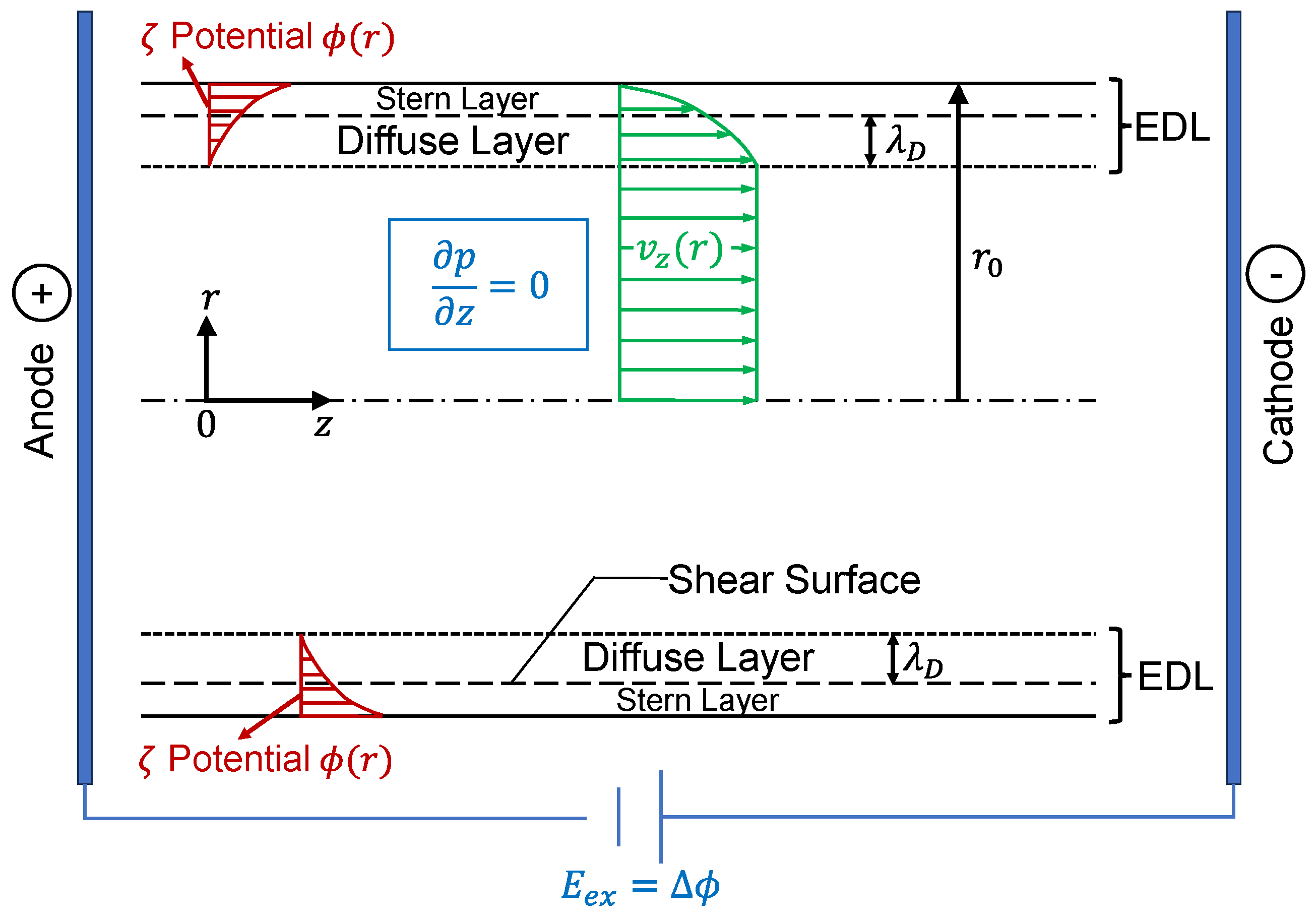
Electroosmotic flow (EOF) is the motion of nanosized boundary layers of an ionized liquid relative to stationary charged surfaces powered by an applied electric field [1]. The liquid nanolayers moving along the walls carry via frictional effects the bulk fluid in the conduit (see Figure 1). In microfluidics, when using micro-flow devices (MFDs) [2,3,4] or biological-micro-electro-mechanical systems (bio-MEMSs) [5,6,7], EOF and other surface-modulated flow applications are most appropriate for small-volume transport (). When higher Reynolds numbers are desired, e.g., for micro-heat sinks, a pressure gradient also needs to be applied. EOF has recently been applied in various industries, including microfluidics, chromatography, drug delivery, biomedical sensors, and electrokinetic pumping [8]. Understanding electroosmotic and pressure-driven flows is also crucial in unveiling the underlying transport phenomena and mechanisms of fluid and drug particles in digestive, respiratory, or urinary tracts, as well as blood vessels [8,9], and other tubular structures in the human body. Therefore, enhancing the fundamental understanding of the principles derived from electroosmotic and pressure-driven flows in microtubes has wide-ranging applications in human health, from the microscopic level of cells and tissues [10] to the macroscopic level of organ systems, offering invaluable insights into the diagnosis, treatment, and understanding of various medical conditions.
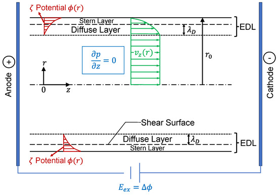
Figure 1.
Sketch of the electroosmotic flow system.
Additionally, the principles of electroosmotic and pressure-driven microtube flow dynamics directly apply to developing lab-on-a-chip (LOC) devices [11,12]. These devices integrate various laboratory functions on a single chip, allowing for the quick and efficient analysis of small volumes of biological fluids, such as blood or saliva [11]. For example, it can be applied to the design of point-of-care (POC) devices for timely diagnosis and treatment for patients [13,14]. It can also be potentially helpful especially in developing LOC devices to mimic human vascular networks, and blood–air barriers in the human respiratory system to investigate lung disease progression, diagnosis, and treatment [8,12,14,15,16,17].
While steady-state electroosmotic and/or pressure-driven flow has been thoroughly investigated analytically [18,19,20,21,22,23], only a few researchers derive analytical solutions for transient EOF in channels or tubes [24,25,26,27,28]. Specifically, previous studies of time-dependent EOFs focused on different microchannel geometrics, typically using semi-analytical approaches or numerical methods [17,24,29,30,31,32,33]. Therefore, what has not been derived is the analytical solution for transient electroosmotic and pressure-driven flows in a microtube.
Thus, this study derived and presented an infinite series as the analytical solution of transient electroosmotic and pressure-driven flows in a microtube. The results are useful for parametric analyses to gain physical insight, to study time-dependent flow effects, and to validate complex computer simulation models. The analytical solutions in electroosmotic and pressure-driven flows offer a precise mathematical representation of fluid behavior under the influence of electrical and pressure gradients. This deepens the understanding of the fluid dynamics in microchannels, which is often more complex due to the interplay of electrical forces, fluid viscosity, and channel geometry. They allow for a systematic analysis of how various parameters (e.g., electric field strength, fluid viscosity, and tube diameter) affect flow characteristics. This is vital in optimizing microfluidic designs for specific applications. By providing a theoretical baseline, the analytical solutions will also be beneficial for guiding the design of experiments and the interpretation of experimental data in electroosmotic and pressure-driven flow studies. They can also serve as benchmarks for validating and refining numerical models that simulate electroosmotic and pressure-driven flows, especially in complex geometries or non-linear regimes where analytical solutions might be difficult to obtain.
2. Materials and Methods
2.1. Governing Equations, Initial Conditions, and Boundary Conditions
The general continuity and momentum equations for the electroosmotic and pressure-driven flow in a cylindrical microtube (see Figure 1) can be given as:
where is the fluid flow velocity, is the pressure, is the fluid density, is the electric charge density, is the fluid kinematic viscosity, and is the external electric field. Assuming constant fluid properties, laminar, and axisymmetric flow, as well as using the Poisson–Boltzmann equation for thin electric double layers (EDLs) and the Debye–Hückel linear approximation [34], Equations (1) and (2) can be simplified as:
where is the external electric field intensity. In Equation (4a), the new body force expression can be further expressed as [34]:
where is the dielectric constant, is the EDL potential, and is the Debye length (see Figure 1). The constant pressure gradient can be expressed as a function of the microtube inlet Reynolds number via the extended Bernoulli equation for laminar flow, i.e.,
where is the area-averaged velocity and is the Reynolds number based on the averaged Poiseuille flow velocity without electroosmotic flow, which is assumed at . = 2 is the tube diameter.
The EDL potential is the solution of the Poisson–Boltzmann (P–B) equation [18,19], which can be given as:
Equation (6) can be reduced for the present one-dimensional (1D) scenario to (see Figure 1):
The initial and boundary conditions for Equation (4a) are:
where is the microtube radius. For Equation (7), the initial and boundary conditions are:
It is worth noting that since the Stern layer of molecular thickness was ignored (see Figure 1), the EDL potential at the wall is approximately equal to the Zeta potential [18,19].
The following dimensionless parameters are introduced to rewrite the governing equations, initial conditions, and boundary conditions, i.e.,
where is the length of the microtube. Substituting Equations (11) and (12) into Equation (4a) yields:
Accordingly, the associated boundary and initial conditions (see Equations (8) and (9)) can be rewritten as:
Similarly, the P–B equation (see Equation (7)) can be nondimensionalized as:
The boundary conditions (see Equation (10)) for the P–B equation can be rewritten as:
Additionally, using Equation (5), the nondimensional term in Equation (13) can be expressed as:
2.2. Analytical Solution
2.2.1. Poisson–Boltzmann (P–B) Equation
The P–B equation was solved first to obtain which was then substituted into the momentum equation for . Noticing that the P–B equation is a modified Bessel equation [35], it was solved with
where is the modified Bessel function of the first kind of order , which is defined as:
When , Equation (18b) yields:
2.2.2. Velocity Profile
Based on the linear momentum equation as well as its boundary conditions and initial condition, the velocity is composed of a steady-state (SS) and a transient part, i.e.,
- Steady-state (SS) Solution
Eliminating the transient term of Equation (13) and substituting Equation (17) into it yields:
where the boundary conditions have been invoked. Introducing the relationship:
where is the dielectric constant, the SS part of the solution for Equation (13) can be given as:
Specifically, when , which means the flow is purely driven by electroosmosis, the SS part of the solution (see Equation (22)) can be simplified as:
- Transient Solution
The transient part of the solution is governed by:
Equation (24a) is subject to the given boundary conditions and initial condition, which can be unified as follows:
By separating variables, the transient part of the solution can be solved and given in the form of
where is the root of and coefficient can be given as:
Therefore, the exact solution for the nondimensionalized axial velocity can be expressed as:
3. Results and Discussion
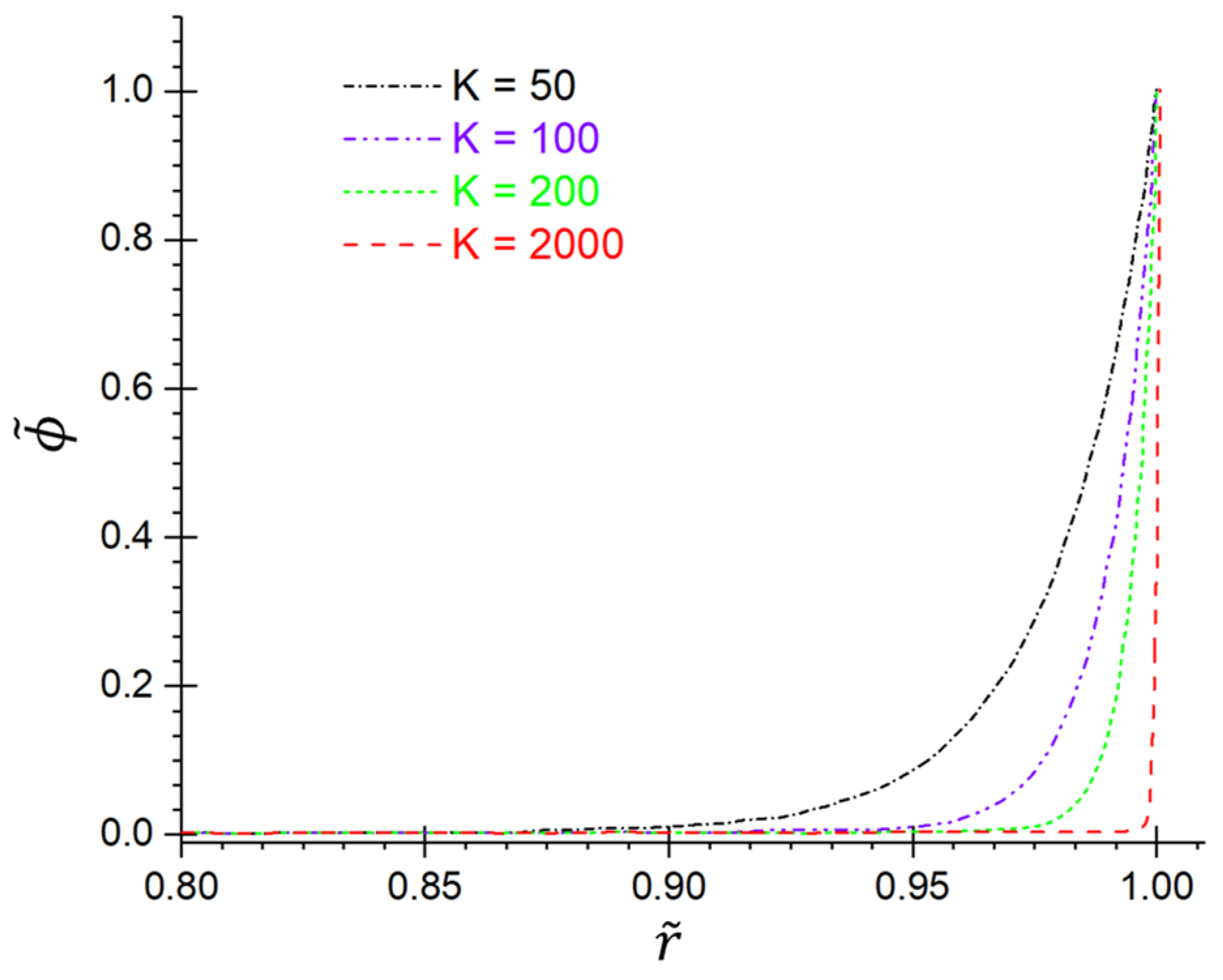
3.1. EDL Potential Profiles
Based on Equation (18a–c), the nondimensionalized EDL potential in the near wall region (i.e., approximately EDL) is shown in Figure 2 with different ratios between the microtube radius and the Debye length, i.e., . For practical applications, understanding the behavior of as a function of can help predict and control the flow characteristics in microfluidic devices. This is crucial for applications involving the precise manipulation of fluids at the microscale, such as in LOCs where electroosmotic flows are used for fluid transport. It can be found that as increases (i.e., the EDL thickness decreases), and the impact region of EDL potential gradually reduces a nano-size surface layer. The Debye length characterizes the scale over which charge carriers screen electrostatic potentials in electrolytes. With higher values, the EDL becomes thinner in comparison to the tube radius . This is visually evident from the potential profiles shown in Figure 2, becoming steeper near the wall and collapsing more quickly to zero as increases. A thinner EDL indicates that the region influenced by surface charges becomes more confined to the wall. It is worth noting that this study assumes that the microtube’s hydraulic diameter is sufficiently large to avoid EDL overlap.
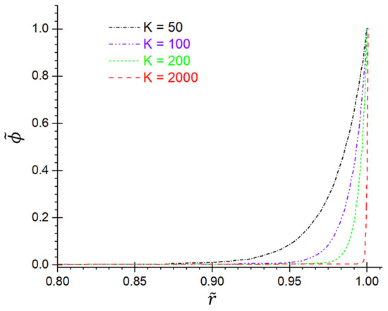
Figure 2.
Near-wall EDL potential distribution along with the radial direction under different values.
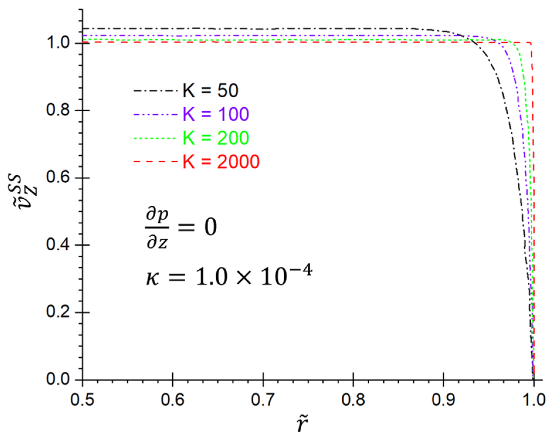
3.2. Pure Electroosmotic Flow
For electroosmotic flow, which is not pressure-driven, the steady-state and fully developed EOF velocity profiles (see Equation (23)) are depicted in Figure 3 as a function of . As indicated in Figure 2, the EDL-affected region changes measurably with and hence the velocity profiles. With large , i.e., and , the velocity distribution along the radial direction is nearly uniform, i.e., , outside of the very thin EDL. With the decrease in which indicates the thickening in EDL, the region of non-uniform near-wall velocity profiles becomes larger. due to the mass conservation, increases with the decrease in . based on the observation in Figure 3, it can be concluded that in pure electroosmotic flow, the steady-state velocity profile across the tube is primarily determined by the distribution of the electric potential within the edl, i.e., the length–scale ratio . typically, in tubes with larger K (thinner edls), the flow becomes more plug-like, with a uniform velocity profile across most of the tube diameter, except very close to the walls where the velocity rapidly adjusts to match the boundary conditions (i.e., zero velocity at the wall due to no-slip condition).
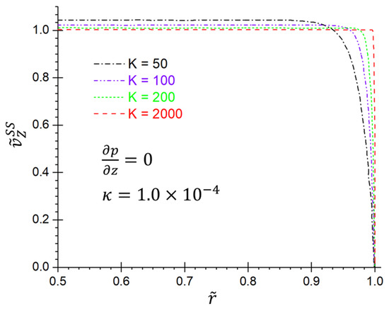
Figure 3.
Velocity profiles with different values for pure electroosmotic flows.
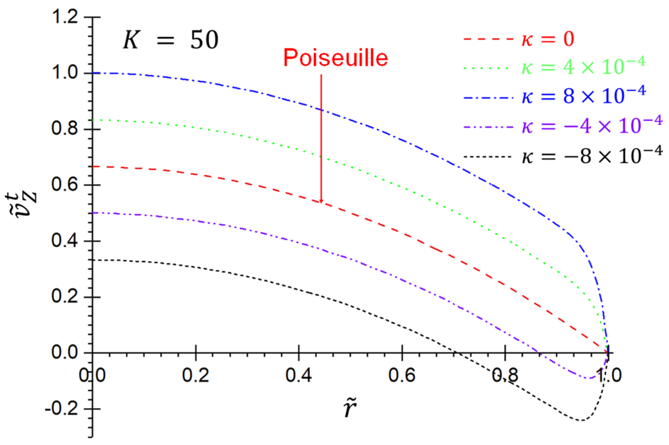
3.3. Electroosmotic and Pressure-Driven Flow
In addition to the length–scale ratio , the electroosmotic slip velocity is also important to characterize microtube flow behaviors for electroosmotic and pressure-driven flow. indicates the ratio of electroosmotic vs. viscous effects, or better as an apparent slip velocity when . Higher values of suggest a dominant electroosmotic effect over viscous effects, influencing the flow characteristics significantly. Specifically, Figure 4 provides a graphical display of Equation (25) with multiple values. It can be observed that the value of determines the nature of the flow, i.e., (1) when , it represents pure pressure-driven flow, where traditional Poiseuille flow is observed, characterized by a parabolic velocity profile with no influence from electroosmotic effects; (2) when , the electroosmotic effect enhances the Poiseuille flow due to the electroosmotic force aiding the pressure-driven flow, resulting in a modified velocity profile that combines both effects; and (3) when , the electroosmosis leads to a backflow near the microtube wall, indicating that the electroosmotic forces oppose the pressure-driven flow, potentially leading to complex flow dynamics. Additionally, the increased electroosmotic effect, signified by a rise in κ, significantly influences the flow velocity distribution within the microtube. This suggests that precise adjustments of electroosmosis can be strategically utilized to manipulate microtube flows, achieving specific objectives in various microfluidic applications. The interpretation of becomes apparent for large -values, such as , as shown in Figure 5. Clearly, for and , the steady-state velocity profile varies from Poiseuille flow with slip at the microtube wall, i.e., m/s. This implies that at high values, even small electroosmotic slip velocities can significantly alter the flow profile.
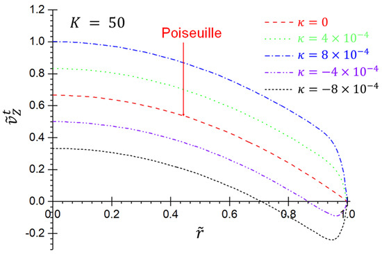
Figure 4.
Steady-state velocity profiles with different values for general case flows with .
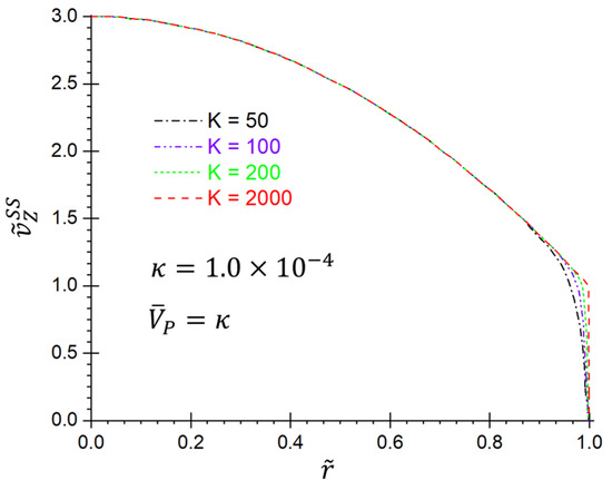
Figure 5.
Steady-state velocity profiles with values for general case flows ().
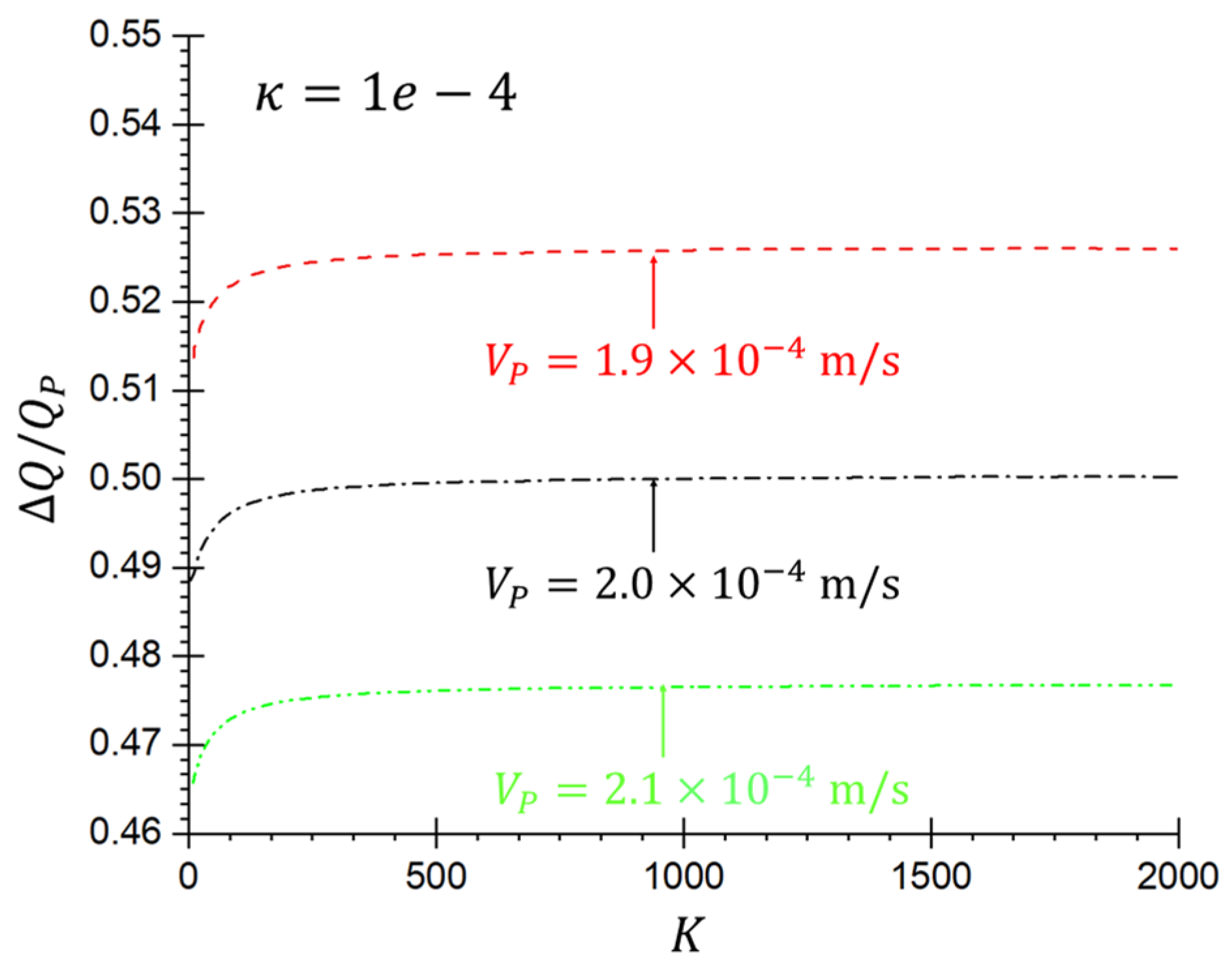
3.4. EOF Flow Rate Gain
As indicated in Figure 4, a positive external electric field increases the electroosmotic flow effect, thereby increasing the flow rate in microtubes. At the same time, a negative one decreases the flow rate. The percentage of flow rate variation due to EOF (i.e., EOF flow rate gain) can be quantified as:
which can be further expressed as:
Assuming , which is the case for NaCl in water, the dependence of on is shown in Figure 6 with multiple values. Clearly, for values larger than , approximately reaches constants. Specifically, when , . Accordingly,
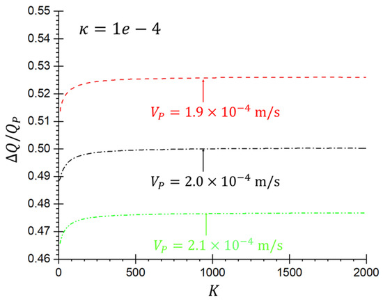
Figure 6.
Percentage of increased flow rate caused by electroosmotic effect when .
Based on Equation (28) and neglecting the non-uniform velocity profile inside EDL, the flow rate gain is just the ratio of apparent slip velocity over the average velocity for Poiseuille flow. Also, as expected, is proportional to the intensity of the external electric field.
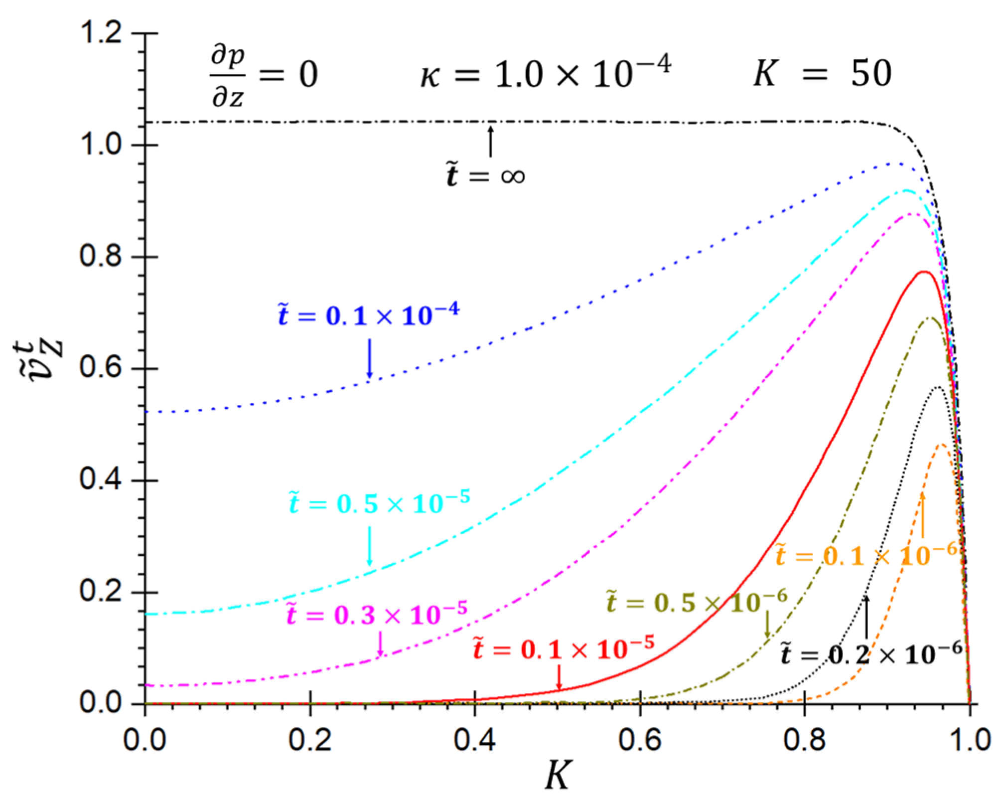
3.5. Transient Velocity Profiles
Recalling that the general case of combined electroosmotic and pressure-driven flows results from a superposition of both driving forces (i.e., external electric field and pressure), the focus here is on transient velocity profile developments due to electroosmosis only. As depicted in Figure 7, at t = 0 s, a constant external electric field is applied, and only the liquid layer in the EDL is set into motion. As the liquid-layer velocity increases with time, radial momentum transfer affects the bulk fluid in the microtube until a steady state is reached, i.e., (see Figure 6). The nondimensionalized time for the velocity profile to reach a steady state is defined as “retarded time”. When , can be expressed as:
or
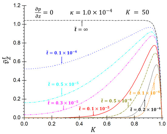
Figure 7.
Velocity profile development with time of pure electroosmotic flow when and .
It can be observed from Equation (29b) that is only related to the hydraulic diameter of the tube and kinematic viscosity , which indicates that the momentum transfer is dominated by viscous forces. As expected, when the fluid viscosity is high, the velocity profile development takes less time to reach a steady state, independent of the average velocity .
3.6. Apparent Slip Velocity
Combined electroosmotic and pressure-driven flows result in velocity profiles very similar to Poiseuille flow with slip boundary conditions if the velocity distribution inside the EDL is neglected (see Figure 5). Therefore, an apparent slip velocity at the wall can be introduced, which is equal to the velocity at , where . Specifically, the apparent slip velocity can be expressed as:
which is only a function of the external electric field intensity and fluid properties (see Equation (2)). Hence, the governing equation of electroosmotic flow can be rewritten as:
but with the key boundary condition:
as well as
3.7. Polynomial Series Approximation of the Steady-State Electroosmotic Flow Solution
Considering Equation (29b), if is of the order of , the characteristic time , which is negligible. Hence, the focus is on the analytical solution of steady electroosmotic flow, i.e.,
utilizing a finite-term polynomial series solution to approximate the analytical solution. Such a polynomial series approximation is more convenient for engineering use than the complex Bessel function solution.
Expressing the Bessel I function in a polynomial series, i.e.,
Equation (34) can be rewritten as:
Allowing an error between and to be less than 5% yields the condition:
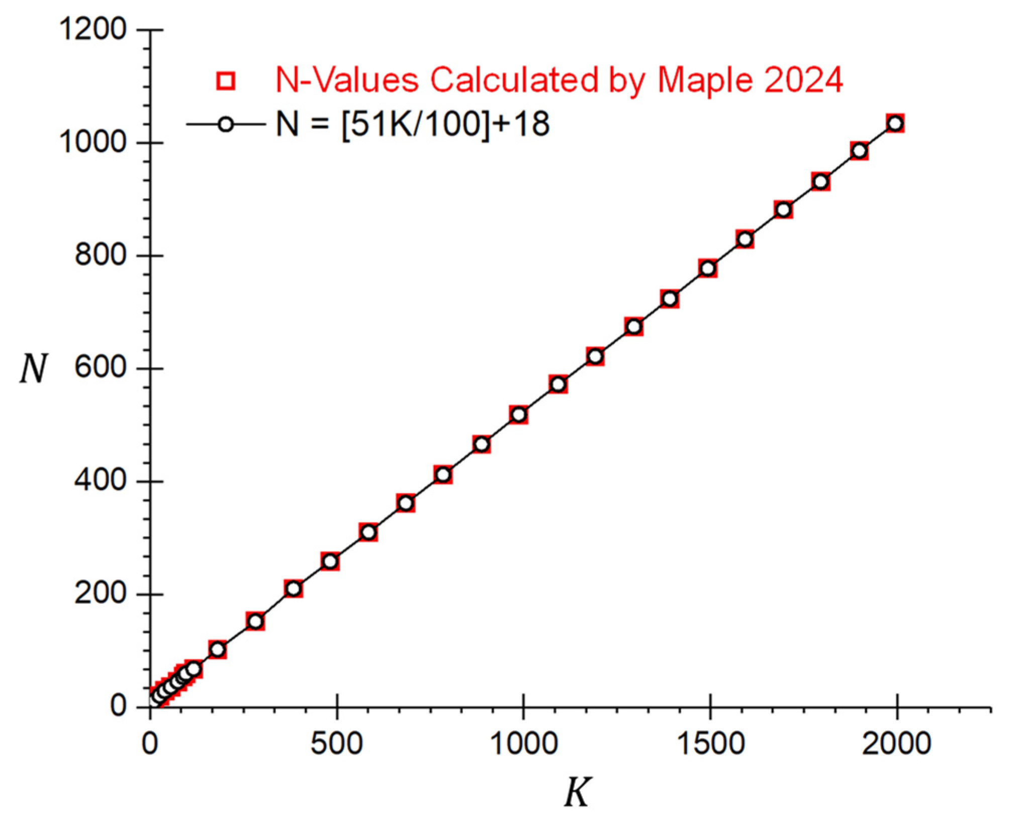
Apparently, is a function of and . To guarantee is large enough to satisfy Equation (37), the following -value estimation is proposed:
where indicates the ceiling function, which is defined as the largest integer not greater than . Equation (38) is plotted in Figure 8, where it fits the calculation data points (calculated by MAPLE 2024, Maplesoft, Waterloo Maple Inc., Waterloo, ON, Canada) perfectly when . At , the estimation value of is larger than the calculation data of which can safely make the error even smaller.

Figure 8.
The relationship between and for a polynomial series approximation solution error less than 5%.
3.8. Shear Stress Distributions for Steady-State Flow
Shear stress can be written as:
Employing Equation (22), can be given as:
Equation (40a) is the general expression of shear stress for electroosmotic and pressure-driven flow, dependent on the parameters and . Introducing characteristic shear stress , the nondimensionalized shear stress can be expressed as:
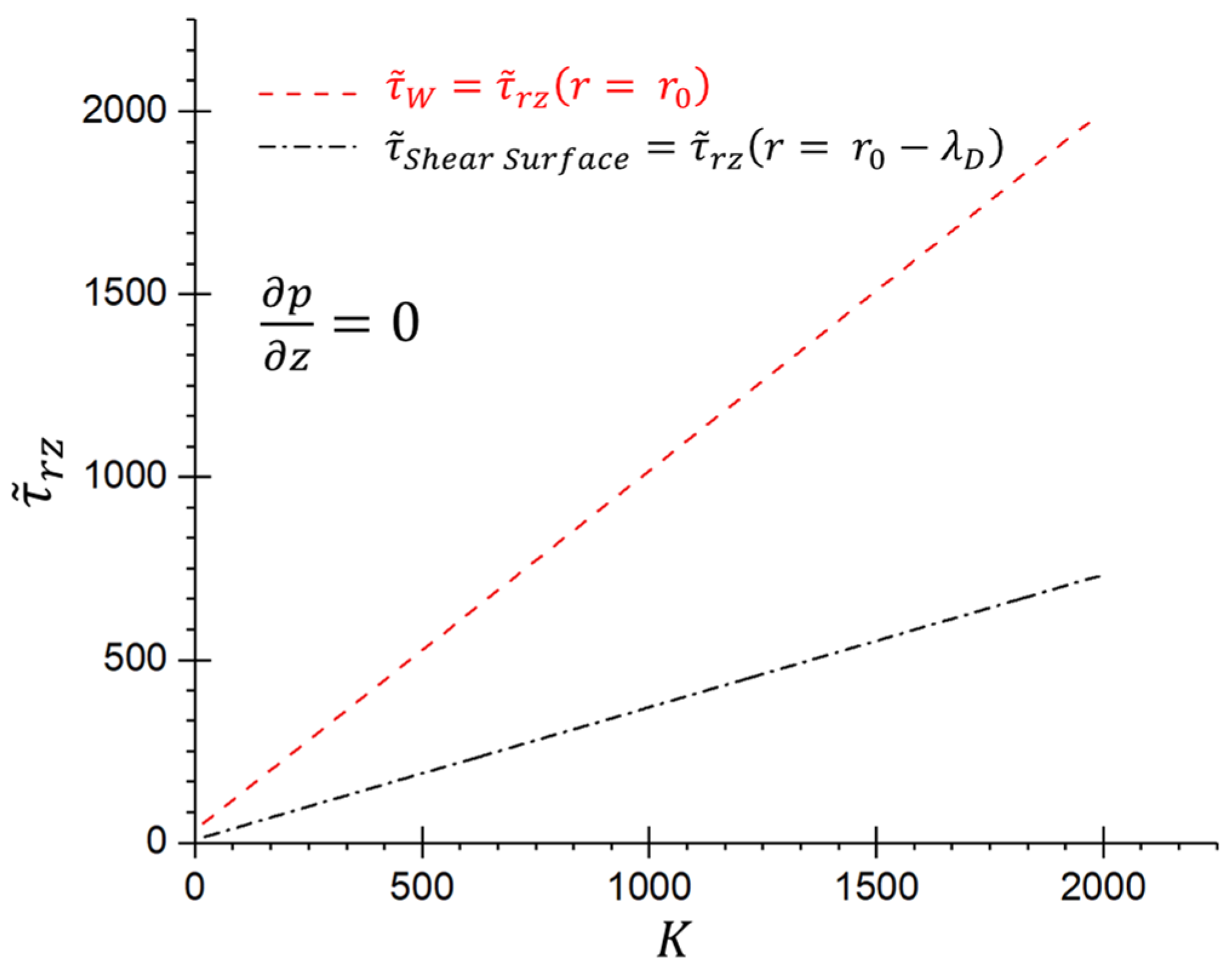
Of interest are the shear stresses at the shear surface (i.e., or ) and at the wall (i.e., or ) (see Figure 1), which can be calculated using Equation (40b) as:
For pure electroosmotic flow, which implies , the graphs of and are shown in Figure 9. With larger values, and increase because the reduced EDL thickness causes steeper velocity gradients at both and . Additionally, for all -values, which aids in the velocity profile development (see Figure 3). It can be observed from Figure 9 that the region in which the shear stress drastically changes (i.e., the shear layer) shrinks when the -value increases.

Figure 9.
Shear stress values at and with different values.
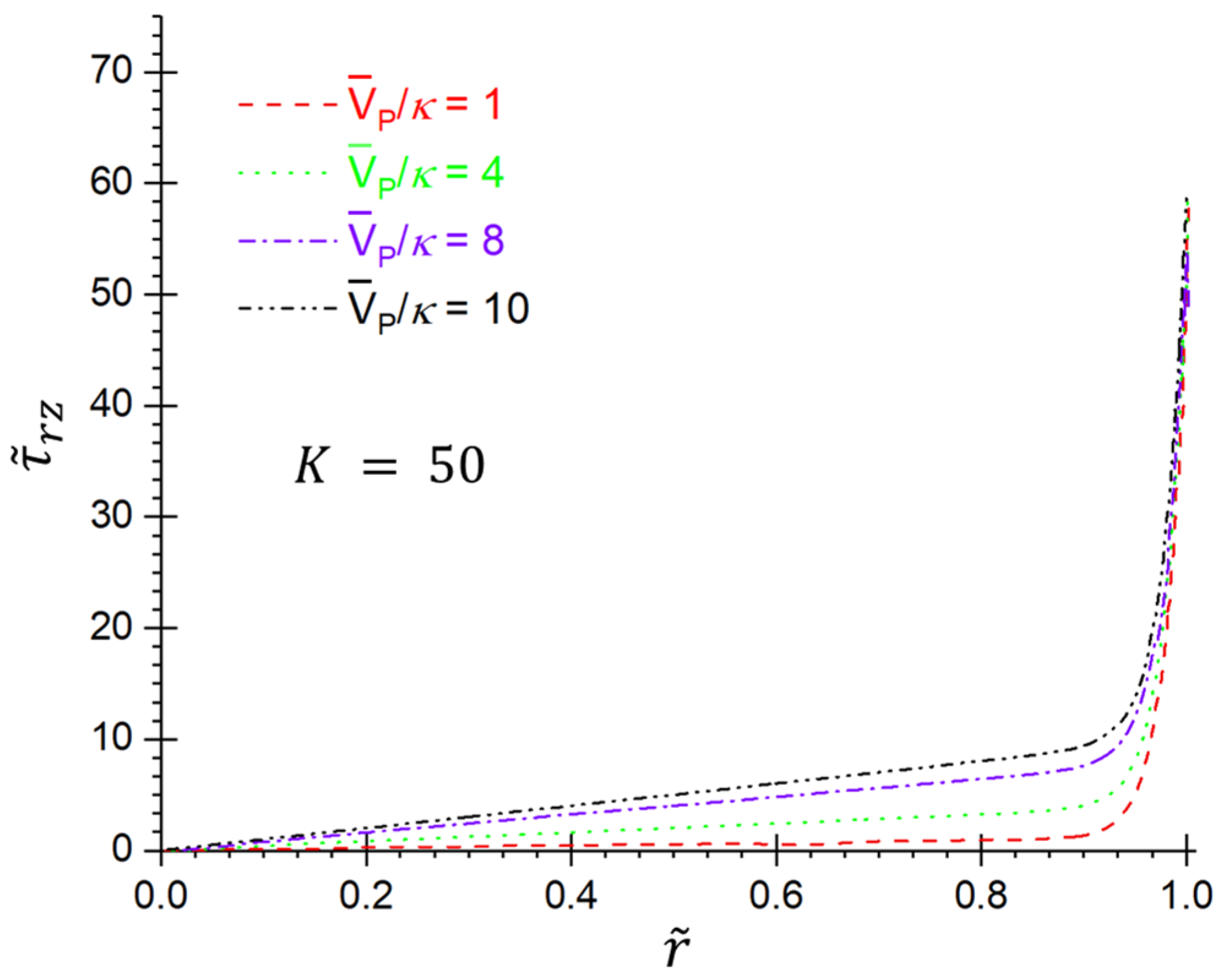
In the more generalized scenario of combined electroosmotic and pressure-driven flows, assuming , the radial shear stress profiles for various ratios are depicted in Figure 10. Inside the EDL, the shear stress remains relatively unchanged with variations in . However, as increases, indicating a steeper shear stress gradient due to the Poiseuille component, a slight increase in shear stress is observed. Outside the EDL, shear stress also rises with increasing values. Notably, at the center line of the microtube (), the shear stress consistently equals zero.

Figure 10.
Shear stress profiles for different -values when .
4. Conclusions
This study derived an analytical solution that can enhance the understanding of electroosmotic and pressure-driven flows in microtubes, with far-reaching implications in the field of microfluidics. The analytical solutions derived illuminate the intricate dynamics of microscale flows, particularly underlining the roles of apparent slip and shear stress distribution. The “retarded time” concept, as introduced and quantified in this work, offers another dimension to the understanding of transient flow behaviors in microscale environments. The practical utility of these findings is further enhanced by the proposed polynomial series approximation for steady-state electroosmotic flows, which simplifies complex calculations for engineering applications. By providing a more profound understanding of flow dynamics at the microscale, this research paves the way for the advanced design and optimization of microfluidic systems. It underscores the interplay between electroosmotic and pressure-driven mechanisms, marking a significant contribution to the theoretical and practical knowledge in microfluidics. This work not only adds to the existing scientific literature but also serves as a valuable guide for future research and development in this dynamic and evolving field.
Author Contributions
Conceptualization, Y.F.; methodology, Y.F.; validation, Y.F., H.Y. and R.L.; formal analysis, Y.F., H.Y. and R.L.; data curation, Y.F., H.Y. and R.L.; writing—original draft preparation, Y.F.; writing—review and editing, Y.F., H.Y. and R.L.; visualization, Y.F. and H.Y.; supervision, Y.F.; project administration, Y.F.; funding acquisition, Y.F. All authors have read and agreed to the published version of the manuscript.
Funding
This research was funded by the U.S. National Science Foundation under grant No. CBET 2120688, and the Oklahoma State University CEAT Engineering Research and Seed Funding Program.
Data Availability Statement
The datasets generated and/or analyzed during the current study are available from the corresponding author upon reasonable request.
Conflicts of Interest
The authors declare no conflicts of interest or financial conflicts, including commercial interests or other competing interests.
References
- Slater, G.W.; Tessier, F.; Kopecka, K. The electroosmotic flow (EOF). In Microengineering in Biotechnology; Humana Press: Totowa, NJ, USA, 2010; pp. 121–134. [Google Scholar]
- Patankar, N.A.; Hu, H.H. Numerical simulation of electroosmotic flow. Anal. Chem. 1998, 70, 1870–1881. [Google Scholar] [CrossRef] [PubMed]
- Gallah, N.; Besbes, K. Electroosmotic micropump analysis for lab on chip water quality monitoring. In Proceedings of the 2016 13th International Multi-Conference on Systems, Signals & Devices (SSD), Leipzig, Germany, 21–24 March 2016. [Google Scholar]
- Gallah, N.; Habbachi, N.; Besbes, K. Design and modelling of droplet based microfluidic system enabled by electroosmotic micropump. Microsyst. Technol. 2017, 23, 5781–5787. [Google Scholar] [CrossRef]
- Alishahi, A.; Vafaie, R.H.; Charmin, A. Numerical Simulation of a Novel Electroosmotic Micropump for Bio-MEMS Applications. Sens. Transducers 2014, 183, 90. [Google Scholar]
- Qaderi, A.; Jamaati, J.; Bahiraei, M. CFD simulation of combined electroosmotic-pressure driven micro-mixing in a microchannel equipped with triangular hurdle and zeta-potential heterogeneity. Chem. Eng. Sci. 2019, 199, 463–477. [Google Scholar] [CrossRef]
- Chen, X.; Cui, D.; Chen, J. Microfluidic Chips for Blood Cell Separation. In On-Chip Pretreatment of Whole Blood by Using MEMS Technology; Bentham Science Publishers: Sharjah, United Arab Emirates, 2012; p. 30. [Google Scholar]
- Ihsan, A.; Ali, A.; Khan, A.U. Thermal analysis of electroosmotic flow in a vertical ciliated tube with viscous dissipation and heat source effects: Implications for endoscopic applications. J. Therm. Anal. Calorim. 2024, 1–15. [Google Scholar] [CrossRef]
- Gandhi, R.; Sharma, B.K.; Mishra, N.K.; Al-Mdallal, Q.M. Computer simulations of EMHD Casson nanofluid flow of blood through an irregular stenotic permeable artery: Application of Koo-Kleinstreuer-Li correlations. Nanomaterials 2023, 13, 652. [Google Scholar] [CrossRef] [PubMed]
- Hui, T.H.; Kwan, K.W.; Yip, T.T.C.; Fong, H.W.; Ngan, K.C.; Yu, M.; Yao, S.; Ngan, A.H.W.; Lin, Y. Regulating the membrane transport activity and death of cells via electroosmotic manipulation. Biophys. J. 2016, 110, 2769–2778. [Google Scholar] [CrossRef]
- Gharib, G.; Bütün, İ.; Muganlı, Z.; Kozalak, G.; Namlı, İ.; Sarraf, S.S.; Ahmadi, V.E.; Toyran, E.; Van Wijnen, A.J.; Koşar, A. Biomedical applications of microfluidic devices: A review. Biosensors 2022, 12, 1023. [Google Scholar] [CrossRef] [PubMed]
- Liu, F.; Jing, D. Combined electroosmotic and pressure driven flow in tree-like microchannel network. Fractals 2021, 29, 2150110. [Google Scholar] [CrossRef]
- Dehghan Manshadi, M.K.; Khojasteh, D.; Mohammadi, M.; Kamali, R. Electroosmotic micropump for lab-on-a-chip biomedical applications. Int. J. Numer. Model. Electron. Netw. Devices Fields 2016, 29, 845–858. [Google Scholar] [CrossRef]
- Chiappetta, C.; Anile, M.; Leopizzi, M.; Venuta, F.; Della Rocca, C. Use of a new generation of capillary electrophoresis to quantify circulating free DNA in non-small cell lung cancer. Clin. Chim. Acta 2013, 425, 93–96. [Google Scholar] [CrossRef] [PubMed]
- Caruso, G.; Musso, N.; Grasso, M.; Costantino, A.; Lazzarino, G.; Tascedda, F.; Gulisano, M.; Lunte, S.M.; Caraci, F. Microfluidics as a novel tool for biological and toxicological assays in drug discovery processes: Focus on microchip electrophoresis. Micromachines 2020, 11, 593. [Google Scholar] [CrossRef]
- Lin, S.H.; Su, T.C.; Huang, S.J.; Jen, C.P. Enhancing the efficiency of lung cancer cell capture using microfluidic dielectrophoresis and aptamer-based surface modification. Electrophoresis 2024, 1–11. [Google Scholar] [CrossRef] [PubMed]
- Jing, D.; Qi, P. Electroosmotic Flow in Fractal Tree-Like Convergent Microchannel Network. Chem. Eng. Technol. 2024, 47, 923–931. [Google Scholar] [CrossRef]
- Karniadakis, G.E.; Beskok, A.; Gad-el-Hak, M. Micro flows: Fundamentals and simulation. Appl. Mech. Rev. 2002, 55, B76. [Google Scholar] [CrossRef]
- Nguyen, N.-T.; Wereley, S.T.; Shaegh, S. Fundamentals and Applications of Microfluidics; Artech House Inc.: Boston, MA, USA, 2006. [Google Scholar]
- Dutta, P.; Beskok, A. Analytical solution of combined electroosmotic/pressure driven flows in two-dimensional straight channels: Finite Debye layer effects. Anal. Chem. 2001, 73, 1979–1986. [Google Scholar] [CrossRef] [PubMed]
- Banerjee, D.; Mehta, S.K.; Pati, S.; Biswas, P. Analytical solution to heat transfer for mixed electroosmotic and pressure-driven flow through a microchannel with slip-dependent zeta potential. Int. J. Heat Mass Transf. 2021, 181, 121989. [Google Scholar] [CrossRef]
- Zhao, C.; Yang, C. An exact solution for electroosmosis of non-Newtonian fluids in microchannels. J. Non-Newton. Fluid Mech. 2011, 166, 1076–1079. [Google Scholar] [CrossRef]
- Ferrás, L.; Afonso, A.; Alves, M.; Nóbrega, J.; Pinho, F. Electro-osmotic and pressure-driven flow of viscoelastic fluids in microchannels: Analytical and semi-analytical solutions. Phys. Fluids 2016, 28, 093102. [Google Scholar] [CrossRef]
- Chang, C.C.; Wang, C.Y. Starting electroosmotic flow in an annulus and in a rectangular channel. Electrophoresis 2008, 29, 2970–2979. [Google Scholar] [CrossRef]
- Dutta, P.; Beskok, A. Analytical solution of time periodic electroosmotic flows: Analogies to Stokes’ second problem. Anal. Chem. 2001, 73, 5097–5102. [Google Scholar] [CrossRef] [PubMed]
- Jian, Y.; Yang, L.; Liu, Q. Time periodic electro-osmotic flow through a microannulus. Phys. Fluids 2010, 22, 042001. [Google Scholar] [CrossRef]
- Guo, X.; Qi, H. Analytical solution of electro-osmotic peristalsis of fractional Jeffreys fluid in a micro-channel. Micromachines 2017, 8, 341. [Google Scholar] [CrossRef] [PubMed]
- Zhao, M.; Wang, S.; Wei, S. Transient electro-osmotic flow of Oldroyd-B fluids in a straight pipe of circular cross section. J. Non-Newton. Fluid Mech. 2013, 201, 135–139. [Google Scholar] [CrossRef]
- Luo, W.-J. Transient electroosmotic flow induced by AC electric field in micro-channel with patchwise surface heterogeneities. J. Colloid Interface Sci. 2006, 295, 551–561. [Google Scholar] [CrossRef]
- Aboelkassem, Y. Computational and theoretical model of electro-osmotic flow pumping in a microchannel with squeezing walls. Phys. Fluids 2023, 35, 052011. [Google Scholar] [CrossRef]
- Ali, N.; Hussain, S.; Ullah, K.; Bég, O.A. Mathematical modelling of two-fluid electro-osmotic peristaltic pumping of an Ellis fluid in an axisymmetric tube. Eur. Phys. J. Plus 2019, 134, 141. [Google Scholar] [CrossRef]
- Ghorbani, S.; Jabari Moghadam, A.; Emamian, A.; Ellahi, R.; Sait, S.M. Numerical simulation of the electroosmotic flow of the Carreau-Yasuda model in the rectangular microchannel. Int. J. Numer. Methods Heat Fluid Flow 2022, 32, 2240–2259. [Google Scholar] [CrossRef]
- Jing, D.; Qi, P. The Optimal Branch Width Convergence Ratio to Maximize the Transport Efficiency of the Combined Electroosmotic and Pressure-Driven Flow within a Fractal Tree-like Convergent Microchannel. Fractal Fract. 2024, 8, 279. [Google Scholar] [CrossRef]
- Park, H.; Lee, J.; Kim, T. Comparison of the Nernst–Planck model and the Poisson–Boltzmann model for electroosmotic flows in microchannels. J. Colloid Interface Sci. 2007, 315, 731–739. [Google Scholar] [CrossRef]
- Asmar, N.H. Partial Differential Equations with Fourier Series and Boundary Value Problems; Courier Dover Publications: Upper Saddle River, NJ, USA, 2016. [Google Scholar]

Disclaimer/Publisher’s Note: The statements, opinions and data contained in all publications are solely those of the individual author(s) and contributor(s) and not of MDPI and/or the editor(s). MDPI and/or the editor(s) disclaim responsibility for any injury to people or property resulting from any ideas, methods, instructions or products referred to in the content. |
© 2024 by the authors. Licensee MDPI, Basel, Switzerland. This article is an open access article distributed under the terms and conditions of the Creative Commons Attribution (CC BY) license (https://creativecommons.org/licenses/by/4.0/).