Toward Scale-Adaptive Subgrid-Scale Model in LES for Turbulent Flow Past a Sphere

Abstract

This study explores the dynamics of turbulent flow around a sphere at a Reynolds number of $\mathcal{R}e={10}^3$ using large-eddy simulation, focusing on the intricate connection between vortices and strain within the recirculation bubble of the wake. Employing a relatively new subgrid-scale modeling approach based on scale adaptivity, this research implements a functional relation to compute $k_{\mathrm{sgs}}$ that encompasses both vortex-stretching and strain rate mechanisms essential for the energy cascade process. The effectiveness of this approach is analyzed in the wake of the sphere, particularly in the recirculation bubble, at the specified Reynolds number. It is also evaluated in comparison with two different subgrid-scale models through detailed analysis of the coherent structures within the recirculation bubble. These models—scale-adaptive, k-Equation, and dynamic k-Equation—are assessed for their ability to capture the complex flow dynamics near the wake. The findings indicate that while all models proficiently simulate key turbulent wake features such as vortex formation and kinetic energy distribution, they exhibit unique strengths and limitations in depicting specific flow characteristics. The scale-adaptive model shows a good ability to dynamically adjust to local flow conditions, thereby enhancing the representation of turbulent structures and eddy viscosity. Similarly, the dKE model exhibits advantages in energy dissipation and vortex dynamics due to its capability to adjust coefficients dynamically based on local conditions. The comparative analysis and statistical evaluation of vortex stretching and strain across models deepen the understanding of turbulence asymmetries and intensities, providing crucial insights for advancing aerodynamic design and analysis in various engineering fields and laying the groundwork for further sophisticated turbulence modeling explorations.

1. Introduction

Turbulent fluid flow consists of coherent structures and random fluctuations [1]. One of the main problems in simulating turbulent flow past a bluff body is how to capture the near-wake region behind a solid body appropriately [2,3]. The solid body causes a significant disturbance in the flow regime, generating a viscous layer, flow separation, and intermittency in its vicinity [4]. The flow separation in the near-wake region leads to a recirculation bubble suppressing the turbulent flow with a substantial straining effect, causing a negative mean velocity profile in this region. This effect, along with the intermittency in the turbulent flow field, requires a numerical approach to properly capture the dynamic nature of the bluff body flows. In a large-eddy simulation (LES) of turbulent flow around bluff bodies like a sphere, understanding the interplay between vortices and strain is critical for an effective approximation of the flow, particularly in the vicinity of the bluff body (i.e., the recirculation bubble). Vortex stretching, which represents the vortices in the flow field, is a pivotal mechanism that influences the energy cascade from larger to smaller scales [5,6,7,8] and is known to impact enstrophy production in the flow, which intrinsically reflects the strength of the vorticity field. Positive vortex stretching is typically associated with an increase in enstrophy and can contribute to a decrease in strain, aligning with the understanding that turbulence enhances mixing and disorder within the flow [9]. Strain self-amplification, on the other hand, plays a significant role in sustaining and increasing strain within turbulent flows, denoting the process where the strain field intensifies itself, which can be a consistent feature in the cascade process of turbulence energy [9].

In the wake of a bluff body, especially in the recirculation bubble, strain self-amplification tends to increase the straining effect [4]. A subgrid-scale (SGS) modeling approach in LES, which merely considers strain self-amplification, leads to a rise in eddy viscosity in this region. Paradoxically, this area experiences turbulence suppression, creating an expectation of reduced eddy viscosity. This dichotomy emphasizes the need for a nuanced approach to model eddy viscosity that not only captures the effects of strain, but also accounts for vortex-stretching phenomena. Therefore, an approach is required to adapt or adjust the length scale to local flow characteristics in space and time. In SGS modeling, it is shown that eddy viscosity is aligned with characteristic turbulence kinetic energy and can be written as ${\nu }_{\mathrm{sgs}}=c_k\Delta \sqrt{k_{\mathrm{sgs}}}$. An intriguing idea could be to utilize a technique to update eddy viscosity spatially and temporally for an LES of turbulent flow. Some dynamic variants of SGS models update the eddy viscosity in accordance to the local properties of fluid flow by dynamically adapting the constant coefficient. To this end, this group of SGS models solves a transport equation to update the turbulent kinetic energy $k_{\mathrm{sgs}}$ accordingly [10,11,12]. These models have shown efficacy in adjusting eddy viscosity in response to the local dynamics of the flow [13], offering a more comprehensive representation of the complex interactions within turbulent wakes [14]. A relatively new approach was recently proposed to approximate eddy viscosity dynamically [15,16] through employing a functional relation for $k_{\mathrm{sgs}}$. A key feature of the scale-adaptive SGS model is to consider both the “strain tensor” and the “rotation tensor”, which allows dynamical adaption of the energy dissipation rate (${\epsilon }_{\Delta }$) as the characteristic length- and time-scale varies in a highly intermittent turbulent flow field. This model has already been meticulously tested for the atmospheric boundary layer [15,17] and discussed statistically for a synthetic turbulent flow field [16].

The dynamic transport equation SGS model solves a transport equation for $k_{\mathrm{sgs}}$ and dynamically adjusts model coefficients using procedures like the Germano identity [11]. The dynamic adjustment is more explicitly calculated through the solution of an additional partial differential equation. However, the scale-adaptive SGS model adjusts the eddy viscosity merely using a functional relation that incorporates both strain and vorticity tensors to link the subgrid-scale turbulent kinetic energy to local flow properties directly through a predefined functional relationship. The transport-equation-based SGS models are relatively more sensitive to mesh quality because they rely on solving an extra PDE for $k_{\mathrm{sgs}}$ [18,19]. Although the dynamic variants of these SGS models mitigate some of this sensitivity by dynamically adjusting model coefficients based on local flow properties, it still depends on mesh resolution for accurate local adjustments. In contrast, a functional relation-based SGS model such as a SA model is less dependent on mesh quality [20]. This model dynamically adjusts the eddy viscosity using local flow characteristics without solving an additional equation, making it relatively independent of mesh resolutions to some extent.

The extensive research into bluff body dynamics, through both experimental [13,21,22,23,24,25,26] and computational studies [15,16,17,27,28,29,30,31,32,33,34] underscores the understanding of the coherent motions dynamic behavior inside the recirculation zone moving downstream in the wake of the bluff body [1,9,35]. Recirculation bubbles are critical phenomena in fluid dynamics, characterized by their ability to influence the aerodynamic and hydrodynamic performance of various structures significantly. In aerodynamics, recirculation bubbles are pivotal in determining the drag and lift characteristics of vehicles [36,37,38,39]. Ahmed et al. [36] demonstrated how varying rear slant angles on a generic vehicle body affects the development and behavior of wake flows, which are closely associated with recirculation bubbles. These bubbles often dictate the pressure distribution around the body, impacting overall aerodynamic efficiency. Similarly, in aerospace engineering, the effects of recirculation bubbles on aerofoil performance are explored, particularly at low Reynolds numbers [40,41]. Collectively, these studies illustrate the diverse implications of recirculation bubbles across various engineering fields [42,43,44,45,46,47,48] and emphasize the importance of understanding coherent motions and turbulent characteristics within the recirculation bubble and in the wake of a bluff body. Large-scale and coherent structures, prominently forming in the massively separated flows over wing surfaces, critically impact phenomena like the flutter of large, flexible wind turbines [49,50]. Understanding the wake behind a bluff body such as a sphere can therefore be essential for assessing the aerodynamic and hydrodynamic behaviors of bluff bodies in contexts ranging from wind turbine performance to the design of underwater robotics and the impact of extreme weather on structures [15,32,51,52]. Previous studies have examined bluff bodies in steady flows, noting significant changes with variations in Reynolds numbers and flow angles. Yet, in-depth explorations of accelerated wakes and their complex aerodynamics have been primarily confined to simple flows past isothermal or heated cylinders [33,34,53,54,55]. Moreover, it is established that the coherent structures in the wake of a sphere differ significantly from those behind other bluff bodies such as circular cylinders, presenting unique challenges and opportunities for detailed flow analysis [56,57]. The literature indicates that various approaches have been considered to capture the unsteadiness of the aerodynamic load on a static sphere, providing reliable correlations to calculate fluid forces and field fluctuations [13,27,58] as well as quantitative measurement of high-order metrics [23,28,59]. These efforts and their collective scientific results can enable us to continue our journey toward improving our understanding, especially of how different length scales and time scales are generated and interact in a turbulent flow [60].

Considering that the cornerstone of turbulence modeling is the assumption of the energy cascade by coherent larger motions and the smaller random fluctuations [61,62], the current research attempts to contribute further to understanding of the role of vortex stretching and strain self-amplification in the recirculation zone of turbulent flow past a sphere at $\mathcal{R}e={10}^3$. At this Reynolds number, the recirculation bubble consists of the shear layer and the shedding mechanisms dominated by a transition from laminar to turbulent flow [30,33], which provides a flow field that, in the presence of axisymmetric geometry, dismisses the complexity of high Reynolds regimes. The reason behind choosing a sphere is that it is an ideal geometry for studying flow past a solid body and recirculation bubble due to its simplicity, symmetry, and well-documented behavior. The axisymmetric shape of the sphere simplifies modeling and analysis, allowing for a clear examination of fundamental flow phenomena such as vortex shedding and wake formation, focusing on the recirculation region. Additionally, the sphere’s relevance to practical applications and its versatility across different Reynolds numbers make it a valuable subject for both experimental and computational fluid dynamics studies. Therefore, this research aims to contribute to understanding the coherent structures in the recirculation zone of a sphere and as they move outside the recirculation zone into highly intermittent turbulent regions.

The paper is organized as follows. In Section 2, a brief mathematical background of LES and the different subgrid-scale models are discussed. Section 3 is divided into three subsections: Section 3.1 presents a mesh sensitivity analysis and then compares the selected mesh resolution with available data in the literature; Section 3.2 and Section 3.3 discuss the results of the scale-adaptive SGS model in detail, where the resolved Reynolds stress, coherent structures, pressure coefficient, Q-criteria, energy spectra, and some statistical analysis of the subgrid-scale parameters are illustrated among three different SGS modeling approaches, which are discussed in the next section.

2. Large-Eddy Simulation Framework

We initiate our exploration by presenting the numerical simulation framework for turbulent flow, focusing on the governing equations that model incompressible fluid flows. In LES, the intricate spatial and temporal evolution of fluid flow is encapsulated through the filtered Navier–Stokes equations as

$$\frac{\partial {\overline{u}}_i}{\partial x_i}=0,$$

(1)

$$\begin{array}{cc}\hfill \frac{\partial {\overline{u}}_i}{\partial t}+\frac{\partial {\overline{u}}_i{\overline{u}}_j}{\partial x_j}=& \hfill -\frac{1}{\rho }\frac{\partial \overline{p}}{\partial x_i}+\nu \frac{\partial }{\partial x_j}\left(\frac{\partial {\overline{u}}_i}{\partial x_j}+\frac{\partial {\overline{u}}_j}{\partial x_i}\right)\hfill \\ \hfill & -\frac{\partial {\tau }_{ij}}{\partial x_j}+\varphi \left(\mathbf{x}\right)P_i,\hfill \end{array}$$

(2)

where $\overline{·}$ denotes the filtered quantities, $u_i$ represents the ith component of velocity, and p denotes pressure. $\rho$ and $\nu$ are fluid density and the kinematic viscosity, respectively. The direct-forcing immersed boundary method, utilized for simulating the sphere, introduces an additional term, $\varphi \left(\mathbf{x}\right)P_i$, in the momentum equation. In this context, $\varphi \left(\mathbf{x}\right)$ serves as a phase indicator, with zero representing fluid and one representing solid. The term $P_i$, defined as $\nu \lambda u_i+\sqrt{\lambda }{u}_i^2$, symbolizes the feedback force exerted by the immersed solid body, encapsulating both frictional drag, $\nu \lambda u_i$, and pressure drag, $\sqrt{\lambda }{u}_i^2$. The coefficient $\lambda$ here represents the resistance factor [63]. This approach, meanwhile, uses no body-fitted mesh for the sphere, allowing for a more flexible computational approach in representing solid objects within the flow field.

In Equation (2), ${\tau }_{ij}=\overline{u_i{u}_j}-{\overline{u}}_i{\overline{u}}_j$ is the subgrid-scale stress. A key challenge in LES involves developing a model that effectively approximates the subgrid-scale stress ${\tau }_{ij}$, thereby ensuring adequate dissipation to represent the energy transfer from larger to smaller eddies. To address this, the classical Smagorinsky SGS model employs an eddy viscosity approach for this approximation [64]. The model asserts that the SGS stress can be represented as

$$\begin{array}{cc}\hfill {\tau }_{ij}-\frac{1}{3}{\tau }_{kk}\approx {\tau }_{ij}^{M,d}=& \hfill -2{(C_s\Delta )}^2\left|\overline{\mathcal{S}}\right|{\overline{\mathcal{S}}}_{ij},\hfill \\ \hfill {\overline{\mathcal{S}}}_{ij}=\frac{\partial {\overline{u}}_i}{\partial x_j}+\frac{\partial {\overline{u}}_j}{\partial x_i}& \hfill ,|\overline{\mathcal{S}}|=\sqrt{2{\overline{\mathcal{S}}}_{ij}{\overline{\mathcal{S}}}_{ij}},\hfill \end{array}$$

(3)

where superscripts M and d stand for the model and the deviatoric or traceless part of the tensor, respectively. Moreover, $C_s$ and $\Delta$ are the Smagorinsky coefficient and the grid filter size, respectively.

2.1. Transport Equation-Based SGS Models

A primary assumption is that it is reasonable to dynamically adjust the energy flux of the SGS motions throughout the entire space–time domain [11]. Following Smagorinsky [64], the eddy viscosity should be prescribed in a way that the appropriate energy flux $-{\tau }_{ij}{\mathcal{S}}_{ij}$; therefore,

$${\tau }_{ij}^{M,d}=2{\nu }_{\tau }{\mathcal{S}}_{ij},$$

(4)

and it is possible to assume that eddy-viscosity ${\nu }_{\tau }$ is aligned with a characteristic turbulence kinetic energy $k_{\mathrm{sgs}}$; hence, it can be written as

$${\nu }_{\tau }=c_k\Delta \sqrt{k_{\mathrm{sgs}}},$$

(5)

where $c_k\Delta$ represents a characteristic length scale. In the classical Smagorinsky model, $k_{\mathrm{sgs}}=2{\Delta }^2{\mathcal{S}}_{ij}{\mathcal{S}}_{ij}$ and $c_k=0.{18}^2$.

In an attempt to implement local adaptivity and backscatter into Smagorinsky-type SGS models, a dynamic equation for $k_{\mathrm{sgs}}$ is proposed [10] as

$$\frac{\partial k_{\mathrm{sgs}}}{\partial t}+{\overline{u}}_j\frac{\partial k_{\mathrm{sgs}}}{\partial x_j}=\frac{\partial }{\partial x_j}\left({\nu }_{\tau }\frac{\partial k_{\mathrm{sgs}}}{\partial x_j}\right)-{\tau }_{ij}{\overline{\mathcal{S}}}_{ij}-\frac{c_{ϵ}}{\Delta }{k}_{\mathrm{sgs}}^{3/2},$$

(6)

where $c_k=0.1$ and $c_{ϵ}=0.93$ are typically considered fixed coefficients for various applications. Here, the calculation of the turbulent kinetic energy $k_{\mathrm{sgs}}$ aims to reach a balance between the energy dissipation and production in the energy cascade process, $\epsilon \equiv c_{ϵ}/\Delta k_{\mathrm{sgs}}^{3/2}={\tau }_{ij}{\mathcal{S}}_{ij}$. By solving this equation, this transport equation-based SGS model (hereafter the k-Eqn model) dynamically determines the local distribution of turbulent kinetic energy, allowing for the eddy viscosity ${\nu }_{\tau }$ to be adjusted based on the local energy levels. Moreover, the steady-state form of Equation (6) leads to the classical Smagorinsky SGS model.

From the classical point of view, turbulent energy is predominantly modeled as cascading from larger scales to smaller ones. However, in reality, energy can also transfer from smaller to larger scales—a phenomenon known as backscatter [9]. Solving Equation (6) in an LES framework can ensure capturing backscatter for situations where local conditions lead to a reverse energy cascade.

There is another variation of the k-Eqn model in which the Germano identity [11] is employed to update $c_k$ and $c_{ϵ}$ dynamically [13]. The dynamic adjustment of these coefficients based on local flow characteristics allows for this model (hereafter the dKE model) to adapt to variations in flow conditions, such as near walls or regions of flow separation, without manual intervention or recalibration of model constants.

2.2. A Scale-Adaptive SGS Model

Based on the scale-similarity hypothesis [65], the subfilter-scale stress, ${\tau }_{ij}^{M,d}$, is equivalent to resolved stresses ${\tau }_{ij}^L=\overline{{\overline{u}}_i{\overline{u}}_j}-{\overline{\overline{u}}}_i{\overline{\overline{u}}}_j$ which accounts for scales between ${\Delta }_{\mathrm{les}}$ and $\alpha {\Delta }_{\mathrm{les}}$. Alam [15] shows that the energy flux associated with the Leonard stress ${\tau }_{ij}^L$ reads as

$${\Pi }^L=-{\mathcal{S}}_{ij}{\tau }_{ij}^L=c_k{\Delta }^2\left[-{\mathcal{S}}_{ij}{\mathcal{S}}_{ik}{\mathcal{S}}_{ki}+\frac{1}{4}{\omega }_i{\omega }_j{\mathcal{S}}_{ij}\right].$$

(7)

A negative skewness of strain, ${\mathcal{S}}_{ij}{\mathcal{S}}_{ik}{\mathcal{S}}_{ki}$, along with a positive value of vorticity stretching, ${\omega }_i{\omega }_j{\mathcal{S}}_{ij}$, increases the second invariant of the velocity gradient tensor ${\mathcal{Q}}_g$ while decreasing the third invariant of the velocity gradient tensor ${\mathcal{R}}_g$. Therefore, it is thus evident that the stretching of vorticity extracts energy as large-scale strain is enhanced [15].

Based on dimensional reasoning [16,66], a functional relation is formulated that maps the space of velocity gradient tensor to the space of turbulence kinetic energy. Thus, the turbulent kinetic energy $k_{\mathrm{sgs}}$ can be obtained through the following expression:

$$k_{\mathrm{sgs}}=\frac{{\Delta }^2{(\frac{1}{2}{\mathcal{S}}_{ij}{\omega }_j{\mathcal{S}}_{ij}{\omega }_k+\frac{1}{6}{\left({\mathcal{G}}_{ij}{\mathcal{G}}_{ij}\right)}^2)}^3}{{[{\left({\mathcal{S}}_{ij}{\mathcal{S}}_{ij}\right)}^{5/2}+{(\frac{1}{2}{\mathcal{S}}_{ij}{\omega }_j{\mathcal{S}}_{ij}{\omega }_k+\frac{1}{6}{\left({\mathcal{G}}_{ij}{\mathcal{G}}_{ij}\right)}^2)}^{5/4}]}^2}.$$

(8)

Several similar investigations support the mathematical justification of Equation (8) [67,68,69]. For clarity, we write down the scale adaptive form of the subgrid-scale stress:

$${\tau }_{ij}-\frac{1}{3}{\tau }_{kk}{\delta }_{ij}=c_k\Delta \sqrt{k_{\mathrm{sgs}}}{\mathcal{S}}_{ij},$$

(9)

where $k_{\mathrm{sgs}}$ is instantaneously learned from the available velocity data. Parameter $c_k$ can be estimated from DNS data of homogeneous isotropic turbulence [16]. The modeled stress is adapted dynamically as the strain is adjusted and vortex tubes are stretched.

3. Results and Discussion

3.1. Mesh Sensitivity Analysis

We consider turbulent flow past a sphere at $\mathcal{R}e={10}^3$. For this, a computational domain is considered with dimensions of $x\in [-6D,26D]$, $y\in [-4D,4D]$, and $z\in [-4D,4D]$ and the immersed boundary of the sphere is located at $(x,y,z)=(0,0,0)$ (see Figure 1). For the discretization of this computational domain, a Cartesian structured uniform mesh is employed, and a mesh sensitivity analysis is performed to choose a proper mesh resolution. At the inlet of this domain, a uniform velocity field $(u/U,v/U,w/U)=(1,0,0)$ is considered. However, a pressure-based boundary condition is used for its outlet. Moreover, all the numerical data in this section and the following ones are obtained at $tU/D=1000$, which equals over 100 vortex-shedding cycles. It is worth mentioning that we use an in-house developed code for the scale-adaptive SGS model and direct-forcing immersed boundary with OpenFOAM solvers to run our simulations.

In this section, a mesh sensitivity analysis is presented using four different mesh resolutions. For all mesh configurations, we use a second-order finite volume discretization of the governing flow equations, and the time step is adjusted to ensure that the maximum Courant number remains below $C_{max}\le 1.25$. A numerical verification of the selected mesh resolution is also demonstrated in comparison with the data published in the literature. For this comparison, quantities such as time-averaged streamwise velocity and its fluctuation, the pressure coefficient, and the skin friction on the boundary of the sphere are considered. To select a proper mesh resolution for the LES of turbulent flow in this paper, different mesh resolutions are considered, as shown in

Table 1. Detail of different mesh resolutions used for mesh sensitivity analysis.

	${\mathit{N}}_{\mathit{CVs}}$	${\mathit{N}}_{\mathit{x}}\times {\mathit{N}}_{\mathit{y}}\times {\mathit{N}}_{\mathit{z}}$	${\mathbf{\Delta }}_{\mathit{x}}={\mathbf{\Delta }}_{\mathit{y}}={\mathbf{\Delta }}_{\mathit{z}}$
mesh 1	442,368	$192\times 48\times 48$	$0.08333$
mesh 2	1,048,576	$256\times 64\times 64$	$0.06250$
mesh 3	2,048,000	$320\times 80\times 80$	$0.05000$
mesh 4	8,388,608	$512\times 128\times 128$	$0.03125$

. To run the mesh sensitivity using scale-adaptive LES at $\mathcal{R}e={10}^3$, mean streamwise velocity and its fluctuation are considered to be compared. Moreover, Figure 1 shows how the mean streamwise velocity profile is affected by the no-slip boundary condition on the spherical region in this domain. As shown in this figure, the mean streamwise velocity is zero on the grid points occupied by the immersed solid body (i.e., the sphere).

Using the mentioned computational setup above, the mean streamwise velocity $\langle {\overline{u}}_x\rangle$ and its corresponding resolved Reynolds stress $\langle u_{\mathrm{rms}}^{\prime }\rangle /U$$\langle u_{\mathrm{rms}}^{\prime }\rangle$ are obtained (see Figure 2) for the different mesh resolutions mentioned in Table 1. In this paper, $\overline{u}$ is the streamwise component of the filtered velocity (see Equation (2)) and $u_{\mathrm{rms}}^{\prime }$ is the root mean square of resolved Reynolds stress in the streamwise direction. Also, $\langle ·\rangle$ is defined as a time-averaged quantity which is averaged over total simulation time (i.e., $tU/D=1000$). Mesh 1 has the lowest computational cost among the other meshes; however, it lacks acceptable accuracy in comparison with Mesh 4 as the finest resolution in this analysis. As presented in Figure 2, Mesh 3 maintains very close numerical results to Mesh 4 with relatively low grid resolution. In this mesh sensitivity analysis, our focus is on the near-wake area, especially on the recirculation bubble zone which is defined as the streamwise distance from the rear end of the sphere to the location in the flow field where the mean streamwise velocity changes sign. The dotted line in Figure 2 shows where the sign of the velocity changes. In this region, Mesh 3 obviously has a fairly good agreement with Mesh 4, which is the finest grid resolution with about 8.4 million grid points.

Now that Mesh 3 has shown acceptable results in our mesh sensitivity analysis, let us see the numerical accuracy of this mesh resolution in comparison with available data. To achieve this, the mean streamwise velocity and the resolved Reynolds stress are compared with published data in Figure 3. In Figure 3a, the mean streamwise velocity is compared with the experimental data from Wu and Faeth [24], the DNS result from Rodriguez et al. [33], and the LES result of Tomboulides and Orszag [27], as well as the result of the vortex-penalization (VP) method published by Mimeau et al. [31]. The mean streamwise velocity obtained by the present result using Mesh 3 shows good agreement with the DNS and experimental data, especially in the recirculation bubble zone. The DNS result is reported to be obtained by a mesh with a $9.6\times {10}^6$ grid point [33]. Figure 3b presents the fluctuation of the mean streamwise velocity for scale-adaptive LES using Mesh 3 in comparison with experimental data, DNS, and LES results. The present result shows good agreement with DNS and LES in the literature. However, all numerical results have a noticeable discrepancy with the experimental data, which can be caused due to integration time, mesh properties, and/or numerical schemes.

The pressure coefficient ($C_p$) on the surface of the sphere is calculated using

$$C_p=\frac{p-p_{\infty }}{p_0-p_{\infty }},$$

(10)

where p and $p_{\infty }$ are the instantaneous pressure at each cell center and the free-stream pressure (or the inlet pressure), respectively. Also, $p_0$ is the stagnation pressure, which is measured at the very front point of the sphere where the fluid comes to rest. In the absence of a body-fitted mesh and utilizing the direct-forcing immersed boundary method to represent the sphere within the computational domain, the calculation of the pressure coefficient ($C_p$) is performed using the cells that contain the sphere boundary. The pressure at each cell center (p) within these boundary cells is used to approximate the pressure on the sphere surface. In Figure 4a, $C_p$ is shown in comparison with DNS and experimental data at $\mathcal{R}e={10}^3$ in the literature. This figure shows that scale-adaptive LES is in agreement with the published data.

In addition to the pressure coefficient, let us consider the skin friction coefficient on the surface of the sphere, which is defined as follows:

$$C_f=\frac{{\tau }_w}{\rho U^2\mathcal{R}{e}^{0.5}},$$

(11)

where ${\tau }_w$, $\rho$, and U are the skin shear stress on the surface of the sphere, the density of free stream fluid, and the free stream velocity, respectively. Figure 4b compares the skin friction coefficient obtained by the scale-adaptive LES at $\mathcal{R}e={10}^3$ with two DNS results, one obtained at $\mathcal{R}e={10}^3$ [33], and another obtained at $\mathcal{R}e=5\times {10}^3$ [70]. The current method agrees with both DNS results, as demonstrated in this figure. Although the current method is simulated at $\mathcal{R}e={10}^3$, it is still possible to compare it to DNS results with a higher Reynolds number since Schlichting [71] showed that dramatic changes in Reynolds numbers have a slight impact on the variation of the skin friction coefficient. allowing for us to compare it on different Reynolds numbers, as shown in Figure 4b.

Considering that a non-body-fitted mesh is utilized for representing the sphere in the computational field, it is also critical to check the value of the viscous length or viscous sublayer thickness, ${\delta }_{\nu }=\nu /u_{\tau }$, where $u_{\tau }$ is friction velocity and $\nu$ is kinematic viscosity. This is necessary to determine whether the resolution of the mesh near-wall is fine enough to resolve the flow. Given that the kinematic viscosity is $\nu ={10}^{-3}$ and the friction velocity is about $u_{\tau }=0.15$, the viscous length is about $6\times {10}^{-3}$. Since ${\delta }_{\nu }$ is less than the mesh size $\Delta$, it presents a challenge for accurately resolving the near-wall region using non-body-fitted meshes. However, the current scale-adaptive-based framework shows good agreement for pressure coefficient and skin friction coefficient despite the mesh size being larger than the viscous length.

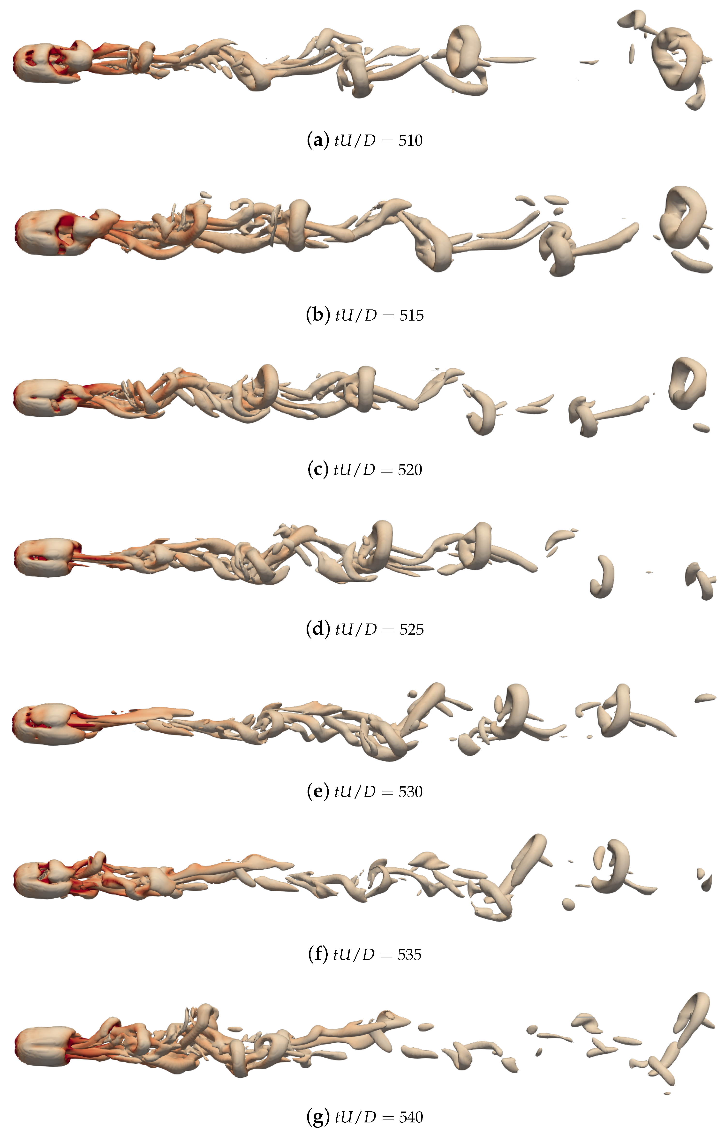
3.2. Dynamic Behavior of Flow in the Wake

To study the dynamic behavior of turbulent flow in the wake of the sphere, we consider utilizing a visualization technique. To this end, we use the Q-criterion method [72], which identifies vortices as flow regions with the positive second invariant of the velocity gradient tensor. This method focuses on the characteristics of the velocity gradient tensor, ${\mathcal{G}}_{ij}$, which can be decomposed into its symmetric part, $\mathcal{S}$ (strain tensor), and its skew-symmetric part, $\Omega$ (the rotation or vorticity tensor). The Q-criterion defines a vortex as a region in the flow where the norm of the rotation tensor exceeds that of the strain tensor.

$$Q=\frac{1}{2}{(\Vert \Omega \Vert }^2-{\Vert \mathcal{S}\Vert }^2)$$

(12)

Here, ${\parallel \Omega \parallel }^2$ represents the square of the magnitude of vorticity, indicating local rotation, and ${\parallel \mathcal{S}\parallel }^2$ is the magnitude of the strain rate, indicating deformation of the fluid elements. A positive Q indicates a dominance of rotation over strain, which is characteristic of a vortex.

The ${\lambda }_2$ criterion [73] is another method for identifying vortex cores. It is based on the eigenvalues, ${\lambda }_1$, ${\lambda }_2$, and ${\lambda }_3$, of the symmetric part of the tensor ${\mathcal{S}}^2+{\Omega }^2$. The eigenvalues are ordered such that ${\lambda }_1\ge {\lambda }_2\ge {\lambda }_3$. Regions where ${\lambda }_2$ is negative are identified as vortical. Unlike the Q-criterion, which considers the overall balance between rotation and strain, the ${\lambda }_2$ method focuses specifically on the plane of maximum shear, providing a more localized view of vorticity. Therefore, the Q-criterion method seems to be more suitable in our case since we are looking for the excess of vorticity in a global sense in the flow field.

Figure 5 illustrates the development of vortical structures in the wake of the sphere at $\mathcal{R}e={10}^3$ from $tU/D=510$ to $tU/D=540$. This series effectively captures the dynamic and complex process of vortex formation and shedding in turbulent flow. The first frame (see Figure 5a) shows an initial instability directly behind the sphere, where small vortical structures begin to form. This is likely the onset of flow separation, where the boundary layer detaches from the surface of the sphere, leading to the formation of a recirculation zone directly behind it. As these instabilities grow (see Figure 5b), they elongate and start to coil, breaking down into more complex structures. This breakdown is indicative of the transition from laminar to turbulent flow characteristics within the wake. The structures then evolve into clearer vortex-shedding patterns (see Figure 5c), where distinct vortices are shed alternately from either side of the wake. This pattern is reminiscent of the von Kármán vortex street, commonly observed in bluff body flows. In Figure 5c–f, the vortices move downstream and continue to interact and merge, growing in size and complexity. The interaction among these vortices within the wake is a key feature of turbulent flow, contributing to the mixing and dispersion of such flows. Eventually, the vortices break down further and dissipate as they move farther from the sphere (see Figure 5g). In this sequence, the recirculation bubble is implied by the initial formation and subsequent motion of vortices. It forms due to the separation of the boundary layer and is sustained by the ongoing shedding of vortices. Some of the instabilities observed, particularly associated with the recirculation bubble, may indicate Kelvin–Helmholtz instability which occurs due to velocity shears within the fluid. Moreover, the turbulence energy is dissipated through the interaction and breakdown of these vortices. Vortices trapped in the recirculation zone contribute to the turbulence intensity before they are eventually shed downstream.

Table 2. Flow characteristic parameters compared to the data in the literature.

Method	$\mathcal{R}\mathit{e}$	${\overline{\mathit{C}}}_{\mathit{d}}$	${\mathit{\theta }}_{\mathit{sp}}$	$\mathit{L}/\mathit{D}$	$\mathit{St}$
Present	${10}^3$	0.471	101.9	2.284	0.207
VP [31]	${10}^3$	0.485	-	1.991	-
LES [28]	$3.7\times {10}^3$	0.355	90.0	2.622	0.210
DNS [33]	${10}^3$	0.466	101.4	2.285	0.200
LES [27]	${10}^3$	-	102.0	1.700	0.195
Exp [24]	$9.6\times {10}^2$	-	-	2.020	-

provides a comprehensive comparison of flow characteristic parameters to benchmark the current LES approach with the published approaches in the literature. The drag coefficient (${\overline{C}}_d$) is a dimensionless number that quantifies the drag resistance of an object in a fluid environment. It is influenced by the shape of the body, surface roughness, and Reynolds number. Differences in ${\overline{C}}_d$ values across methods underscore variations in computational models or experimental setups. However, the current study shows a good agreement with DNS [33] at the same $\mathcal{R}e={10}^3$. The drag coefficient and the characteristics of the recirculation bubble are interrelated. A larger recirculation bubble generally increases the wake size and drag on the body [74]. The separation angle (${\theta }_{sp}$) indicates where the flow separates from the sphere’s surface, leading to wake formation. It is crucial to understand how the sphere alters the flow field. The provided angles suggest slight variances in flow behavior as captured by different methods. The recirculation bubble length ($L/D$), which is normalized by the diameter of the sphere, shows how long the reversed flow persists behind the sphere before recovering from attaching back or dissipating. This parameter is vital for understanding wake stability and vortex formation. For a flow past a sphere at $\mathcal{R}e={10}^3$, experimental data [24] suggest that the recirculation bubble length is about $2.02$. The current study, along with other LES and DNS studies, shows a good agreement in this regard. The Strouhal number $St=fD/U$, where f is the vortex-shedding frequency, D is the sphere’s diameter, and U is the velocity of the free stream. It is significant in vortex shedding studies and relates the vortex-shedding frequency to the sphere diameter and flow velocity. It is indicative of oscillatory flow patterns, which are crucial for predicting dynamic loads on structures in the flow. The Strouhal numbers are relatively consistent, supporting the reliability of the vortex shedding frequency measurements across different methodologies.

Overall, the present study’s results are closely aligned with the DNS [33], suggesting that the simulation setup effectively captures the complex dynamics of turbulent flow around a sphere. The slight variations in ${\overline{C}}_d$ and ${\theta }_{sp}$ among different methods highlight the sensitivity of these parameters to the nuances of each experimental and computational approach. Notably, the LES by Yun et al. [28] at a higher Re shows a lower ${\overline{C}}_d$ and a reduced separation angle, possibly indicating a shift toward a more streamlined flow as Re increases. The variation in $L/D$ values across different studies underscores the influence of flow dynamics and modeling or experimental techniques on the extent of the recirculation zone.

In

Table 3. Second-order statistics obtained by the current method compared to DNS and LES data in the literature.

	$\mathcal{R}\mathit{e}$	Value	$\mathit{x}/\mathit{D}$	$\mathit{y}/\mathit{D}$
	Max. of streamwise turbulent intensity ($\overline{u_x^{\prime }{u}_x^{\prime }}/U^2$)
Present	${10}^3$	0.057	1.851	0.382
DNS [29]	$3.7\times {10}^3$	0.055	2.606	0.423
LES [75]	${10}^4$	0.063	1.780	0.46
	Max. of crosswise turbulent intensity ($\overline{u_y^{\prime }{u}_y^{\prime }}/U^2$)
Present	${10}^3$	0.041	2.501	0.0
DNS [29]	$3.7\times {10}^3$	0.069	3.090	0.0
LES [75]	${10}^4$	-	-	-
	Max. of Reynolds shear stress ($\overline{u_x^{\prime }{u}_y^{\prime }}/U^2$)
Present	${10}^3$	−0.024	2.189	0.410
DNS [29]	$3.7\times {10}^3$	−0.029	2.565	0.392
LES [75]	${10}^4$	−0.039	2.040	0.390

, the second-order statistics calculated by scale-adaptive LES are compared to the available DNS [29] and LES [75] results in the literature at $\mathcal{R}e=3.7\times {10}^3$ and $\mathcal{R}e={10}^4$, respectively. The maximum value of streamwise turbulent intensity $\overline{u_x^{\prime }{u}_x^{\prime }}/U^2$, crosswise turbulent intensity $\overline{u_y^{\prime }{u}_y^{\prime }}/U^2$, and Reynolds shear stress $\overline{u_x^{\prime }{u}_y^{\prime }}/U^2$ are presented in this table. This comparison demonstrates the dynamic behavior of the flow in the wake of the sphere for different approaches. The main goal of the comparison in this table is to observe where the maximum values of turbulent intensity components and Reynolds shear stress are located. Instead of focusing on the value itself, it is more important to see how the trend is changing, especially for $y/D$. This table demonstrates that the location of the maximum streamwise turbulent intensity diverts from the centerline as the Reynolds number increases. On the other hand, the location of the maximum Reynolds shear stress is moving closer to the centerline.

3.3. Evaluation of Scale-Adaptive SGS Model

In this section, we delve into a comparative analysis of three aforementioned SGS models in Section 2—scale-adaptive (SA), transport equation with constant coefficients (k-Eqn), and transport equation with dynamically calculated coefficients (dKE)—with a particular focus on the turbulent flow behavior within the near-wake region, specifically the recirculation bubble. The k-Eqn model updates the turbulent kinematic energy by solving the momentum equation at each time step, employing fixed coefficients that do not adapt to varying flow conditions across different regions of the flow field. This is modified in the dynamic k-Eqn (dKE) model, which enhances the model prediction of energy dissipation through dynamically calculating the coefficients in Equation (6), thereby allowing for dynamic adjustments of dissipation rate and energy backscatter based on local flow. These two models and the SA model were evaluated using the same computational setup and mesh resolutions described in Section 3.1. This evaluation provides a focused discussion on model efficacy in capturing the complex turbulence characteristics and dynamics within the recirculation bubble.

Figure 6 illustrates the streamlines and coherent structures in the recirculation zones behind a sphere for three SGS models. Such a visualization clarifies the sensitivity of SGS models in predicting the wake behind a sphere. The similarity between streamlines shown in Figure 6a,e suggests that the vortex-stretching principle of the scale-adaptive model accounts for the localized dynamics captured by the dKE model. In other words, the SA model dynamically adjusts the eddy viscosity by learning the local flow conditions through the Helmholtz vortex theorem. According to Equation (6), the energy backscatter influences the eddy viscosity predicted by the k-Eqn model through the flux $-{\tau }_{ij}{\mathcal{S}}_{ij}$ term. In contrast, the dKE model dynamically adjusts the eddy viscosity to account for the energy backscatter.

Figure 7 illustrates a comparative analysis of the streamwise component of mean velocity across these SGS models. In Figure 7a, the mean velocity $\langle u_x\rangle /U$ is plotted along the streamwise which shows how velocity profiles from all models converge near $x/D=2.284$, a point likely signifying the end of the recirculation bubble where flow reattachment begins. This region is characterized by a negative velocity, indicating reverse flow within the bubble. The k-Eqn model predicts a smaller recirculation length relative to the dKE and SA models. This difference can be attributed to the dynamic nature of these models. Both the dKE and SA models incorporate a dynamic approach that allows for them to update the eddy viscosity based on the local properties of the flow. In contrast, the KE model uses fixed coefficients that do not adjust to local flow variations. The consideration of the rotational part of the velocity gradient field in the calculation of SGS models can significantly influence the prediction of the recirculation bubble length. Incorporating this component allows for a more detailed representation of the swirling motions and vortex structures that are prevalent in turbulent flows. Figure 7b presents crosswise velocity profiles at different locations: $x/D=1.6$ (within the recirculation bubble), $x/D=3.0$, and $x/D=5.0$, demonstrating how the flow transitions from reverse to forward as it moves downstream. At $x/D=1.6$, the profiles clearly show negative velocities indicative of the recirculation zone, while at further downstream positions ($x/D=3.0$ and $x/D=5.0$), the velocities are positive, reflecting flow recovery and stabilization. The close alignment of velocity profiles from different models at $x/D=5.0$ suggests a convergence in model predictions as the flow evolves away from the sphere, highlighting the models’ capabilities in capturing the essential dynamics of turbulent wake flows.

Figure 8 compares the pressure coefficient $C_p$ (see Equation (10)) distributions on the surface of a sphere as modeled by SGS models. The coefficients are plotted against angular position $\theta$, revealing a high $C_p$ at the front stagnation point ($\theta =0^{\circ }$) with a sharp decrease towards the rear, indicative of typical flow separation and pressure drop around bluff bodies. While all models show similar trends, there are notable differences towards the wake region ($\theta ={120}^{\circ }–{180}^{\circ }$), where SA shows lesser pressure recovery compared to dKE, suggesting variations in how these models handle wake dynamics and turbulence.

In Figure 9, the streamwise, crosswise, and shear components of the resolved Reynolds stress are shown at different locations in the wake of the sphere. These Reynolds stress components represent turbulent fluctuations in the flow and are crucial for understanding the momentum exchange. Inside the recirculation bubble $x/D=1.6$, we observe that the SA model exhibits relatively symmetrical profiles compared to k-Eqn and dKE models. This behavior in k-Eqn and dKE can be related to their mesh sensitivity, especially in the near-wake region. The dependence of Reynolds stress behavior on flow regime is highlighted in the literature [76]. It is already shown in the literature that as the flow transitions from laminar to turbulent regimes, the Reynolds stress profiles change correspondingly [77]. Nagata et al. [78] thoroughly investigated different flow regimes at $\mathcal{R}e={10}^3$ and concluded that the position of the separation point moves from downstream to upstream as Reynolds number increases under incompressible flows of $\mathcal{R}e\le {10}^3$, and the flow regime changes from fully attached flow to planar–symmetric wake flows. Therefore, it is expected to predict a symmetrical profile in the immediate wake of the sphere, considering that its geometry is simply symmetrical. As the flow progresses downstream, the streamwise component of the resolved Reynolds stress for k-Eqn and dKE remains asymmetrical, while SA keeps the same trend. However, at $x/D=3.0$, the profiles for the crosswise component diverge slightly, with the SA model predicting a marginally higher peak in Reynolds stress. Further downstream at $x/D=5.0$, the discrepancies among the models become more apparent, especially in the streamwise component. The plots shown in Figure 9 indicate that the vortex-stretching principle of the SA model predicts Reynolds stresses with an equivalent accuracy compared to the dynamic models. However, we observe that turbulence prediction is quite sensitive to the choice of methods, including vortex-stretching in SGS modeling, which highlights a novel framework that helps avoid ad hoc parameter adjustment.

In principal, diagonal components measure the resolved turbulent kinetic energy $k_{\mathrm{res}}$ and predicting higher values (as observed in Figure 9) can be interpreted as a higher accuracy. This can be properly investigated for further details through metric $k_{\mathrm{sgs}}/(k_{\mathrm{res}}+k_{\mathrm{sgs}})$, where $k_{\mathrm{res}}=0.5\times (\overline{u_x^{\prime }{u}_x^{\prime }}+\overline{u_y^{\prime }{u}_y^{\prime }}+\overline{u_z^{\prime }{u}_z^{\prime }})$. Pope [35] suggests that a value of this metric that is less than $0.2$ indicates that the energy spectrum is sufficiently resolved. In order to highlight the role of coherent vortices in subgrid-scale turbulence production,

Table 4. Metric $k_{\mathrm{sgs}}/(k_{\mathrm{res}}+k_{\mathrm{sgs}})$ statistical data for different SGS models.

Statistic	SA	k-Eqn	dKE
Mean	0.1074	0.3714	0.2044
Median	0.0076	0.2454	0.0411
STD	0.0767	0.3472	0.2937

and Figure 10 summarize the statistical data and the probability density of the metric. The mean value of this metric is the lowest for the SA model, indicating that the energy spectrum is sufficiently resolved by the SA model compared to other models in the same computational setup. Standard deviation (STD) is also the lowest for SA, implying less variability in the metric for this model, whereas the k-Eqn model has the highest STD, indicating more fluctuation probably due to utilizing globally fixed coefficients.

Plots in Figure 10 highlight distinct behaviors of the metric across these models. For the SA model, the probability density is highly concentrated near zero, indicating that most of the values are very small, suggesting that subgrid-scale turbulence is minimal compared to the resolved turbulence and that the model was able to capture the turbulence properly. In contrast, the k-Eqn model shows a more dispersed distribution, with a notable peak towards higher values close to one, implying significant contributions from subgrid-scale turbulence. The dKE model displays a distribution pattern similar to the SA model but with slightly greater spread, suggesting relatively moderate subgrid-scale turbulence contributions. These visualizations corroborate the statistical data presented in Table 4, where the k-Eqn model exhibits the highest mean and variability in the metric, while the SA model has the lowest. It is worth mentioning that the data used for Table 4 and Figure 10 correspond to the same snapshot of the flow where their coherent structures are shown in Figure 6.

An energy spectra analysis to identify the main frequency corresponding to the large-scale vortex shedding is performed using the Fourier transform of the instantaneous velocity field. Figure 11 shows the energy spectra for the streamwise component of the instantaneous velocity field sampled at different stations in the near-wake region. The first probe for sampling is located at the axisymmetric shear layer at $x/D=1.0$ and $y/D=0.5$ near the rear of the sphere in the recirculation bubble zone. The second one is located at $x/D=5.0$ and $y/D=0.5$, where the transition to turbulence is expected to occur. The energy spectra are calculated using the time series of the instantaneous streamwise velocity over a period of $1000tU/D$ and are illustrated in the normalized frequency format in Figure 11. At both locations, energy spectra curves show good agreement with $k^{-5/3}$ for all SGS models. The peak detected at $x/D=5.0$ and $y/D=0.5$ is not present in the near-wake region, which can be related to the existence of the recirculation bubble zone.

For all three SGS models, one can notice that the instantaneous streamwise velocity displays different frequency contributions depending on the location of sampling the shear layer and in the wake. Indeed, the spectra of velocity for three SGS models located at $x/D=5.0$ and $y/D=0.5$ exhibit a dominant peak. In this figure, the $-5/3$ Kolmogorov’s law is presented as well, which is more visible in the spectra at $x/D=5.0$ and $y/D=0.5$.

Let us now discuss the subgrid-scale statistics and the interaction of the main driving mechanism in the energy cascade for this turbulent flow past a sphere by studying the probability distribution of the instantaneous velocity field and its derivatives. One of the significant results that we expect here is that the probability distribution of vortex stretching and strain skewness is not Gaussian Davidson [1]. This is important since the positive mean value of the vortex stretching comes from the fact that the strain field is strongly negatively skewed [15].

The data presented in

Table 5. Skewness and kurtosis of vortex stretching ${\omega }_i{\omega }_j{\mathcal{S}}_{ij}$ and strain skewness $S_{ij}{S}_{jk}{S}_{ki}$.

	${\mathit{\omega }}_{\mathit{i}}{\mathit{\omega }}_{\mathit{j}}{\mathcal{S}}_{\mathit{ij}}$		${\mathit{S}}_{\mathit{ij}}{\mathit{S}}_{\mathit{jk}}{\mathit{S}}_{\mathit{ki}}$
	Skewness	Kurtosis	Skewness	Kurtosis
SA	23	588	−23	633
K-Eqn	22	552	−22	591
dKE	23	598	−23	643

highlight the skewness and kurtosis for vortex stretching and strain skewness metrics, providing insights into the turbulence characteristics captured by the SA, k-Eqn, and dKE models. Notably, the skewness values indicate the asymmetry of the turbulence fields, whereas the kurtosis values, much higher than three (which would indicate a normal distribution), suggest a significant presence of extreme events in the flow. A positive (or negative) value of skewness can be interpreted as the existence of a longer tail on the right (or left) of the probability distribution. The kurtosis of a probability distribution measures the level of intermittency of a random variable. In this table, the level of intermittency of ${\omega }_i{\omega }_j{\mathcal{S}}_{ij}$ and $S_{ij}{S}_{jk}{S}_{ki}$ for SA and dKE are relatively close due to dynamically updating the eddy viscosity to the local variations in the computational domain.

Figure 12 provides a visualization of the turbulence characteristics captured by three different SGS models through the joint probability distribution functions (JPDFs) of the second ${\mathcal{Q}}_g$ and the third ${\mathcal{R}}_g$ invariants of the velocity gradient tensor ${\mathcal{G}}_{ij}$, alongside their respective probability density of ${\mathcal{R}}_g$. The JPDF of these parameters measures the subgrid-scale dynamics, and the teardrop shape of such a distribution is crucial for understanding the significance of the proposed scale-adaptive model. These plots are instrumental in comparing how each model simulates the turbulent flow behavior, particularly focusing on the anisotropy and intensity of the vortical structures within the near-wake region, including the recirculation bubble. The JPDFs display the frequency of specific ${\mathcal{Q}}_g$ and ${\mathcal{R}}_g$ values, presenting typical teardrop shapes which are indicative of intense vortex dynamics [67]. The SA model demonstrates a narrower distribution focusing on higher ${\mathcal{Q}}_g$ values, suggesting a capture of more intense vortex stretching. In contrast, the k-Eqn and dKE models show a broader spread, indicating a wider range of turbulence scales and more dynamic interactions. The probability density of ${\mathcal{R}}_g$ further outlines the symmetry and skewness in the distribution of its values.

Figure 13 showcases the variations in how the three SGS models, namely SA, k-Eqn, and dKE, depict turbulence dynamics. The plots are structured to compare the interactions of vortical structures and strain effects within the turbulent flow. Figure 13a,c,e illustrate the JPDFs of ${\omega }_i{S}_{ij}{u}_j$, which relate to the intensity of vortex stretching. Figure 13b,d,f, on the other hand, displays the JPDFs of ${\mathcal{Q}}_g$ and ${\mathcal{R}}_g$, offering insights into the distribution of velocity gradient tensor invariants across different flow conditions. These visualizations are indicative of each model’s sensitivity to capturing the complexities of flow separation and reattachment in turbulent regimes, particularly in the wake of bluff bodies where such dynamics are critical for accurate predictions of flow behavior.

4. Conclusions

This study focused on the dynamics of flow in the recirculation bubble in the wake of a sphere at $\mathcal{R}e={10}^3$, emphasizing the critical role of vortex stretching and strain self-amplification. The dynamic behavior of flow past a sphere at $\mathcal{R}e={10}^3$ was simulated using LES with a relatively new SGS modeling approach based on scale-similarity introduced by Leonard [65]. This approach implements a functional relation to obtain $k_{\mathrm{sgs}}$ involving both vortex-stretching and strain rate mechanisms in the energy cascade process. The main idea of using a functional relation to obtain $k_{\mathrm{sgs}}$ with lesser mesh sensitivity was benchmarked against previous studies focusing on the coherent structures in the recirculation bubble. Through the use of three SGS models—scale-adaptive (SA), k-Equation (k-Eqn), and dynamic k-Equation (dKE)—the research examined how these models represent the complex dynamics of turbulence in the near-wake region. These models were evaluated in terms of their capability to capture complex flow characteristics, especially in the recirculation bubble, which is crucial for understanding the aerodynamic properties of bluff bodies. The results demonstrated that all three models effectively simulated the key features of turbulent wakes, such as the formation and behavior of vortices. The dKE model, which solves a transport equation for $\left(k_{\mathrm{sgs}}\right)$ and dynamically adjusts the model coefficients, showed relatively similar to the SA model rather than the k-Eqn model, which keeps the model coefficients constant. One of the drawbacks of the transport equation-based models is that they are calculated through the solution of an additional PDE, making it sensitive to mesh quality. Although the dynamic adjustment of the dKE model helps mitigate some of this sensitivity, accurate local adjustments still depend on mesh resolution, especially in the recirculation bubble, as shown in the resolved Reynolds stress components. The probability density of metric $k_{\mathrm{sgs}}/(k_{\mathrm{res}}+k_{\mathrm{sgs}})$ revealed that the SA model has a high concentration of values near zero, indicating minimal subgrid-scale turbulence compared to resolved turbulence. The dKE model showed relatively moderate subgrid-scale turbulence contributions, while the k-Eqn model showed a more dispersed distribution, suggesting significant subgrid-scale contributions. The statistical analysis of vortex stretching and strain across the models provided deeper insight into turbulence intensities and asymmetries in the flow. These insights are crucial for advancing the understanding of turbulence behavior, which is essential for aerodynamic design and analysis in various engineering applications. This study sets a foundation for future explorations into more sophisticated turbulence models, enhancing the accuracy and reliability of turbulence simulations in complex flow scenarios.

References

1. Davidson, P.A. Turbulence—An Introduction for Scientists and Engineers; Oxford University Press: Oxford, UK, 2004. [Google Scholar]
2. Rodi, W. Turbulence Models and Their Application in Hydraulics: A State of the Art Review; International Association for Hydraulic Research: Madrid, Spain, 1993. [Google Scholar]
3. Schlichting, H.; Gersten, K. Boundary-Layer Theory, 8th ed.; Springer: Berlin/Heidelberg, Germany, 2000. [Google Scholar]
4. Norberg, C. Fluctuations and Structure of the Wake Behind a Bluff Body. Prog. Aerosp. Sci. 2003, 39, 467–510. [Google Scholar]
5. Taylor, G.I. The transport of vorticity and heat through fluids in turbulent motion. Proc. R. Soc. A 1932, 135, 685–702. [Google Scholar] [CrossRef]
6. Taylor, G.I. Production and dissipation of vorticity in a turbulent fluid. Proc. R. Soc. A 1938, 164, 15–23. [Google Scholar] [CrossRef]
7. Onsager, L. Statistical Hydrodynamics. Il Nuovo C. 1949, 6, 279–287. [Google Scholar] [CrossRef]
8. Tennekes, H.; Lumley, J.L. A First Course in Turbulence; MIT Press: Cambridge, MA, USA, 1972. [Google Scholar]
9. Johnson, P.L. On the role of vorticity stretching and strain self-amplification in the turbulence energy cascade. J. Fluid Mech. 2021, 922, A3. [Google Scholar] [CrossRef]
10. Yoshizawa, A. Statistical theory for compressible turbulent shear flows, with the application to subgrid modeling. Phys. Fluids 1985, 29, 2152–2164. [Google Scholar] [CrossRef]
11. Germano, M.; Piomelli, U.; Moin, P.; Cabot, W.H. A dynamic subgrid-scale eddy viscosity model. Phys. Fluids A Fluid Dyn. 1991, 3, 1760–1765. [Google Scholar] [CrossRef]
12. Germano, M. Turbulence: The filtering approach. J. Fluid Mech. 1992, 238, 325–336. [Google Scholar] [CrossRef]
13. Kim, W.; Menon, S. A new dynamic one-equation subgrid-scale model for large eddy simulations. In Proceedings of the 33rd Aerospace Sciences Meeting and Exhibit, Reno, NV, USA, 9–12 January 1995. [Google Scholar] [CrossRef]
14. Meneveau, C. Lagrangian Dynamics and Models of the Velocity Gradient Tensor in Turbulent Flows. Annu. Rev. Fluid Mech. 2011, 43, 219–245. [Google Scholar] [CrossRef]
15. Alam, J. Interaction of vortex stretching with wind power fluctuations. Phys. Fluids 2022, 34, 075132. [Google Scholar] [CrossRef]
16. Hossen, M.K.; Mulayath Variyath, A.; Alam, J.M. Statistical Analysis of Dynamic Subgrid Modeling Approaches in Large Eddy Simulation. Aerospace 2021, 8, 375. [Google Scholar] [CrossRef]
17. Bhuiyan, M.S.; Alam, J. Scale-adaptive turbulence modelling for LES over complex terrain. Eng. Comput. 2020, 38, 1995–2007. [Google Scholar] [CrossRef]
18. Celik, I.B.; Cehreli, Z.N.; Yavuz, I. Index of Resolution Quality for Large Eddy Simulations. J. Fluids Eng. 2005, 127, 949–958. [Google Scholar] [CrossRef]
19. Klein, M. An Attempt to Assess the Quality of Large Eddy Simulations in the Context of Implicit Filtering. Flow Turbul. Combust. 2005, 75, 131–147. [Google Scholar] [CrossRef]
20. Arya, N.; De, A. Effect of Grid Sensitivity on the Performance of Wall Adapting SGS Models for LES of Swirling and Separating–Reattaching Flows. Comput. Math. Appl. 2019, 78, 2035–2051. [Google Scholar] [CrossRef]
21. Achenbach, E. Vortex shedding from spheres. J. Fluid Mech. 1974, 62, 209–221. [Google Scholar] [CrossRef]
22. Kim, H.J.; Durbin, P.A. Observations of the frequencies in a sphere wake and of drag increase by acoustic excitation. Phys. Fluids 1988, 31, 3260. [Google Scholar] [CrossRef]
23. Sakamoto, H.; Haniu, H. A Study on Vortex Shedding From Spheres in a Uniform Flow. J. Fluids Eng. 1990, 112, 386–392. [Google Scholar] [CrossRef]
24. Wu, J.S.; Faeth, G.M. Sphere wakes in still surroundings at intermediate Reynolds numbers. AIAA J. 1993, 31, 1448–1455. [Google Scholar] [CrossRef]
25. Wu, J.S.; Faeth, G.M. Sphere wakes at moderate Reynolds numbers in a turbulent environment. AIAA J. 1994, 32, 535–541. [Google Scholar] [CrossRef]
26. Yarusevych, S.; Sullivan, P.E.; Kawall, J.G. On vortex shedding from an airfoil in low-Reynolds-number flows. J. Fluid Mech. 2009, 632, 245–271. [Google Scholar] [CrossRef]
27. Tomboulides, A.G.; Orszag, S.A. Numerical investigation of transitional and weak turbulent flow past a sphere. J. Fluid Mech. 2000, 416, 45–73. [Google Scholar] [CrossRef]
28. Yun, G.; Kim, D.; Choi, H. Vortical structures behind a sphere at subcritical Reynolds numbers. Phys. Fluids 2006, 18, 015102. [Google Scholar] [CrossRef]
29. Rodriguez, I.; Borell, R.; Lehmkuhl, O.; Segarra, C.D.P.; Oliva, A. Direct numerical simulation of the flow over a sphere at Re = 3700. J. Fluid Mech. 2011, 679, 263–287. [Google Scholar] [CrossRef]
30. Rodriguez, I.; Lehmkuhl, O.; Borrell, R.; Oliva, A. Flow dynamics in the turbulent wake of a sphere at sub-critical Reynolds numbers. Comput. Fluids 2013, 80, 233–243. [Google Scholar] [CrossRef]
31. Mimeau, C.; Mortazavi, I.; Cottet, G.H. Passive control of the flow around a hemisphere using porous media. Eur. J. Mech.-B/Fluids 2017, 65, 213–226. [Google Scholar] [CrossRef]
32. Alam, J.M.; Fitzpatrick, L.P. Large eddy simulation of flow through a periodic array of urban-like obstacles using a canopy stress method. Comput. Fluids 2018, 171, 65–78. [Google Scholar] [CrossRef]
33. Rodriguez, I.; Lehmkuhl, O.; Soria, M.; Gómez, S.; Domínguez-Pumar, M.; Kowalski, L. Fluid dynamics and heat transfer in the wake of a sphere. Int. J. Heat Fluid Flow 2019, 76, 141–153. [Google Scholar] [CrossRef]
34. Marefat, H.A.; Alam, J.; Pope, K. Immersed Boundary Method Implemented in LES for Flow Past a Sphere at Subcritical Reynolds Numbers. In Proceedings of the ASME Fluids Engineering Division’s (FED) Summer Meeting 2022, Toronto, ON, Canada, 3–5 August 2022. [Google Scholar] [CrossRef]
35. Pope, S.B. Turbulent Flows. Meas. Sci. Technol. 2001, 12, 2020–2021. [Google Scholar] [CrossRef]
36. Ahmed, S.R.; Ramm, G.; Faltin, G. Experimental investigation of the flow around a generic vehicle body and its wake development for different rear slant angles. Exp. Fluids 1984, 2, 31–40. [Google Scholar]
37. Zimmermann, R.; Gasteuil, Y.; Bourgoin, M.; Volk, R.; Pumir, A.; Pinton, J.F. Turbulence Induced Lift Experienced by Large Particles in a Turbulent Flow. Phys. Rev. Lett. 2011, 106, 154501. [Google Scholar] [CrossRef] [PubMed]
38. Zimmermann, R.; Gasteuil, Y.; Volk, R.; Bourgoin, M.; Pumir, A.; Pinton, J.F. Rotational Intermittency and Turbulence Induced Lift Experienced by Large Particles in a Turbulent Flow. J. Phys. Conf. Ser. 2011, 318, 052027. [Google Scholar] [CrossRef]
39. Rastello, M.; Marié, J.L.; Lance, M. Drag and lift forces on clean spherical and ellipsoidal bubbles in a solid-body rotating flow. J. Fluid Mech. 2011, 682, 434–463. [Google Scholar] [CrossRef]
40. Mueller, T.J.; Batill, S.M. Effects of recirculation bubbles on aerofoil performance at low Reynolds numbers. AIAA J. 1982, 20, 457–463. [Google Scholar] [CrossRef]
41. Mo, J.o.; Rho, B.s. Characteristics and Effects of Laminar Separation Bubbles on NREL S809 Airfoil Using the γ-Reθ Transition Model. Appl. Sci. 2020, 10, 6095. [Google Scholar] [CrossRef]
42. Dey, S.; Raikar, R.V. Recirculation zones and their impact on bridge pier scour under steady and unsteady flow conditions. J. Hydraul. Eng. 2007, 133, 989–1003. [Google Scholar]
43. Carolus, T.H.; Sturm, B.; Lakshminarayana, B. Influence of Blade Number on Flow Recirculation and Fan Performance. J. Turbomach. 2008, 130, 031005. [Google Scholar] [CrossRef]
44. De Kat, R.; van Oudheusden, B.W. Instantaneous planar pressure determination from PIV in turbulent flow. Exp. Fluids 2012, 52, 1089–1106. [Google Scholar] [CrossRef]
45. Wei, L.; Pohl, P.I.; Crowe, A. The role of recirculation zones in improving the efficiency of raceway ponds for microalgae cultivation. Algal Res. 2015, 12, 367–376. [Google Scholar] [CrossRef]
46. Sanjose, M.; Moreau, S.; Roger, M. Noise prediction and control in high-speed jets. Aerosp. Sci. Technol. 2020, 106, 106050. [Google Scholar]
47. Carolus, T.; Schröder, T. Noise generated by airfoils and fans operating in non-uniform inflow conditions. J. Sound Vib. 2021, 495, 115861. [Google Scholar]
48. Blocken, B.; Toparlar, Y. A review on aerodynamic drag and lift in sports: Cycling, running, skiing, and swimming. J. Wind Eng. Ind. Aerodyn. 2021, 209, 104550. [Google Scholar]
49. Barnes, C.J.; Visbal, M.R. On the role of flow transition in laminar separation flutter. J. Fluids Struct. 2018, 77, 213–230. [Google Scholar] [CrossRef]
50. Akhter, M.Z.; Omar, F.K. Review of Flow-Control Devices for Wind-Turbine Performance Enhancement. Energies 2021, 14, 1268. [Google Scholar] [CrossRef]
51. Korkmaz, F.C.; Güzel, B. Water entry of cylinders and spheres under hydrophobic effects; Case for advancing deadrise angles. Ocean Eng. 2017, 129, 240–252. [Google Scholar] [CrossRef]
52. Zeinali, B.; Ghazanfarian, J. Turbulent flow over partially superhydrophobic underwater structures: The case of flow over sphere and step. Ocean Eng. 2020, 195, 106688. [Google Scholar] [CrossRef]
53. Bhattacharyya, S.; Chattopadhyay, H.; Biswas, R.; Ewim, D.R.E.; Huan, Z. Influence of Inlet Turbulence Intensity on Transport Phenomenon of Modified Diamond Cylinder: A Numerical Study. Arab. J. Sci. Eng. 2020, 45, 1051–1058. [Google Scholar] [CrossRef]
54. Murmu, S.C.; Bhattacharyya, S.; Chattopadhyay, H.; Biswas, R. Analysis of heat transfer around bluff bodies with variable inlet turbulent intensity: A numerical simulation. Int. Commun. Heat Mass Transf. 2020, 117, 104779. [Google Scholar] [CrossRef]
55. Rodriguez, I.; Lehmkuhl, O.; Soria, M. On the effects of the free-stream turbulence on the heat transfer from a sphere. Int. J. Heat Mass Transf. 2021, 164, 120579. [Google Scholar] [CrossRef]
56. Yazdi, M.E.; Khoshnevis, A.B. Comparing the wake behind circular and elliptical cylinders in a uniform current. SN Appl. Sci. 2020, 2, 994. [Google Scholar] [CrossRef]
57. Takamure, K.; Kato, H.; Uchiyama, T. Wake characteristics of sphere with circular uniaxial through-hole arranged perpendicularly to streamwise direction. Powder Technol. 2023, 415, 118175. [Google Scholar] [CrossRef]
58. Squire, H.B. Modern Development in Fluid Dynamics, 3rd ed.; Springer: Berlin/Heidelberg, Germany, 1950; Volume 2. [Google Scholar]
59. Ong, L.; Wallace, J. The velocity field of the turbulent very near wake of a circular cylinder. Exp. Fluids 1996, 20, 441–453. [Google Scholar] [CrossRef]
60. Sircar, A.; Kimber, M.; Rokkam, S.; Botha, G. Turbulent flow and heat flux analysis from validated large eddy simulations of flow past a heated cylinder in the near wake region. Phys. Fluids 2020, 32, 125119. [Google Scholar] [CrossRef]
61. Chung, D.; Pullin, D. Large-eddy simulation and wall modelling of turbulent channel flow. J. Fluid Mech. 2009, 631, 281–309. [Google Scholar] [CrossRef]
62. Trias, F.X.; Folch, D.; Gorobets, A.; Oliva, A. Building proper invariants for eddy-viscosity subgrid-scale models. Phys. Fluids 2015, 27, 065103. [Google Scholar] [CrossRef]
63. Whitaker, S. The Forchheimer Equation: A Theoretical Development. Transp. Porous Media 1996, 25, 27–61. [Google Scholar] [CrossRef]
64. Smagorinsky, J. General circulation experiments with the primitive equations: I. The basic experiment. Mon. Weather Rev. 1963, 91, 99–164. [Google Scholar] [CrossRef]
65. Leonard, A. Energy Cascade in Large Eddy Simulations of Turbulent Fluid Flow. Adv. Geophys. 1974, 18, 237–248. [Google Scholar] [CrossRef]
66. Alam, J.M. Toward a Multiscale Approach for Computational Atmospheric Modeling. Mon. Weather Rev. 2011, 139, 3906–3922. [Google Scholar] [CrossRef]
67. Dallas, V.; Alexakis, A. Structures and dynamics of small scales in three-dimensional magnetohydrodynamic turbulence. Phys. Fluids 2013, 25, 105106. [Google Scholar]
68. Buxton, O.R.H.; Breda, M.; Chen, X. The effects of Reynolds number and Stokes number on particle-pair relative velocity in isotropic turbulence: A systematic experimental study. J. Fluid Mech. 2017, 817, 1–20. [Google Scholar] [CrossRef]
69. Danish, M.; Meneveau, C. Variance of force distributions in homogeneous isotropic turbulence. Phys. Rev. Fluids 2018, 3, 044604. [Google Scholar] [CrossRef]
70. Seidl, V.; Muzaferija, S.; Perić, M. Parallel DNS with Local Grid Refinement. Appl. Sci. Res. 1997, 59, 379–394. [Google Scholar] [CrossRef]
71. Schlichting, H. Boundary Layer Theory, 7th ed.; Springer: Berlin/Heidelberg, Germany, 1979. [Google Scholar]
72. Hunt, J.C.R.; Wray, A.A.; Moin, P. Eddies, stream and convergence zones in turbulent flows. In Proceedings of the Studying Turbulence Using Numerical Simulation Databases, 2. Proceedings of the 1988 Summer Program, Stanford, CA, USA, 22–27 July 1988. [Google Scholar]
73. Jeong, J.; Hussain, F. On the identification of a vortex. J. Fluid Mech. 1995, 285, 69–94. [Google Scholar] [CrossRef]
74. Schlichting, H.; Gersten, K. Boundary-Layer Theory, 9th ed.; Springer: Berlin/Heidelberg, Germany, 2017. [Google Scholar]
75. Constantinescu, G.; Squires, K.D. Numerical investigations on the effect of subgrid models in LES of the flow past a circular cylinder at Reynolds number 3900. Phys. Fluids 2003, 15, 2021–2039. [Google Scholar] [CrossRef]
76. Zanoun, E.S.; Dewidar, Y.; Egbers, C. Reynolds number dependence of azimuthal and streamwise pipe flow structures. J. Fluid Mech. 2023, 943, A11. [Google Scholar] [CrossRef]
77. Johnson, T.A.; Patel, V.C. Flow past a sphere up to a Reynolds number of 300. J. Fluid Mech. 1999, 378, 19–70. [Google Scholar] [CrossRef]
78. Nagata, T.; Nonomura, T.; Takahashi, S.; Fukuda, K. Direct numerical simulation of subsonic, transonic and supersonic flow over an isolated sphere up to a Reynolds number of 1000. J. Fluid Mech. 2020, 898, A18. [Google Scholar] [CrossRef]
Figure 1. A zoomed—in view of the computational domain with the time—averaged streamwise velocity profile at different locations in the near wake of the sphere. The black arrow shows the direction of fluid flow.
Fluids 09 00144 g001
Figure 2. (a) Time—averaged streamwise velocity and (b) its corresponding resolved Reynolds stress u rms / U along the x direction for different mesh resolutions.
Fluids 09 00144 g002
Figure 3. (a) Time—averaged streamwise velocity u ¯ / U and (b) its corresponding resolved Reynolds stress u rms / U along the x direction compared to Exp [24], DNS [33], LES [27], and VP [31].
Fluids 09 00144 g003
Figure 4. (a) The pressure coefficient on the surface of the sphere compared to experiment [22] and DNS [33] at R e = 10 3 . (b) The skin—friction coefficient on the surface of the sphere at R e = 10 3 in comparison with DNS result at R e = 10 3 [33] and another DNS result at R e = 5 × 10 3 [70].
Fluids 09 00144 g004
Figure 5. Instantaneous vortical structures in the wake of the sphere at R e = 10 3 . In this illustration, time advances from t U / D = 510 (a) to t U / D = 540 (g).
Fluids 09 00144 g005
Figure 6. Streamlines (a,c,e) and coherent structures (b,d,f) in the recirculation zone illustrated in the wake of the sphere for (a,b) SA, (c,d) k-Eqn, and (e,f) dKE. Blue and red shadings show low- and high-vorticity zones, respectively.
Fluids 09 00144 g006
Figure 7. The streamwise component of the mean velocity for scale-adaptive, k-Eqn, and dKE SGS models: (a) in the streamwise direction, (b) at three different locations in the wake of the sphere.
Fluids 09 00144 g007
Figure 8. Pressure coefficient C p on the boundary of the sphere compared for different SGS models.
Fluids 09 00144 g008
Figure 9. Streamwise (ac), crosswise (df), and shear (gi) components of the resolved Reynolds stress at different locations in the wake of the sphere.
Fluids 09 00144 g009
Figure 10. Probability density of metric k sgs / ( k res + k sgs ) compared between SA (a), k-Eqn (b), and dKE (c).
Fluids 09 00144 g010
Figure 11. Energy spectra of the instantaneous streamwise velocity at different locations in the wake of the sphere: a comparison for different SGS models.
Fluids 09 00144 g011
Figure 12. Joint probability distribution function of Q g and R g for a comparison between SA (a), k-Eqn (c), and dKE (e). The probability density of R G for a comparison between SA (b), k-Eqn (d), and dKE (f).
Fluids 09 00144 g012
Figure 13. Joint probability distribution function of ω i S i j ω j and S i j S j k S k i , as well as that of Q s and R s for a comparison between SA (a,b), k-Eqn (c,d), and dKE (e,f).
Fluids 09 00144 g013