Abstract
Understanding the flow instabilities encountered by the turbocharger compressor is an important step toward improving its overall design for performance and efficiency. While an experimental study using Particle Image Velocimetry was previously conducted to examine the flow field at the inlet of the turbocharger compressor, the present work complements that effort by analyzing the flow structures leading to stall instability within the same impeller. Experimentally validated three-dimensional computational fluid dynamics predictions are carried out at three discrete mass flow rates, including 77 g/s (stable, maximum flow condition), 57 g/s (near peak efficiency), and 30 g/s (with strong reverse flow from the impeller) at a fixed rotational speed of 80,000 rpm. Large stationary stall cells were observed deep within the impeller at 30 g/s, occupying a significant portion of the blade passage near the shroud between the suction surface of the main blades and the pressure surface of the splitter blades. These stall cells are mainly created when a substantial portion of the inlet core flow is unable to follow the impeller’s axial to radial bend against the adverse pressure gradient and becomes entrained by the reverse flow and the tip leakage flow, giving rise to a region of low-momentum fluid in its wake. This phenomenon was observed to a lesser extent at 57 g/s and was completely absent at 77 g/s. On the other hand, the inducer rotating stall was found to be most dominant at 57 g/s. The entrainment of the tip leakage flow by the core flow moving into the impeller, leading to the generation of an unstable, wavy shear layer at the inducer plane, was instrumental in the generation of rotating stall. The present analyses provide a detailed characterization of both stationary and rotating stall cells and demonstrate the physics behind their formation, as well as their effect on compressor efficiency. The study also characterizes the entropy generation within the impeller under different operating conditions. While at 77 g/s, the entropy generation is mostly concentrated near the shroud of the impeller with the core flow being almost isentropic, at 30 g/s, there is a significant increase in the area within the blade passage that shows elevated entropy production. The tip leakage flow, its interaction with the blades and the core forward flow, and the reverse flow within the impeller are found to be the major sources of irreversibilities.
1. Introduction
Downsizing internal combustion engines along with turbocharging is an effective approach for reducing carbon dioxide emissions from vehicles to mitigate global warming [1]. A turbocharger comprises a radial turbine driven by exhaust enthalpy flow connected on the same shaft to a centrifugal compressor that provides compressed air to the engine. Under certain engine operating conditions, the turbocharger faces challenges, however, due to instabilities encountered by its centrifugal compressor, primarily stall and surge [2]. While stall adversely affects the compressor’s aerodynamic performance and efficiency, deep surge, which is characterized by large amplitude pressure and flow rate fluctuations, results in drastic deterioration of compressor performance and may lead to complete mechanical failure of the turbocharger [3]. The noise generated due to these instabilities (reaching 170 dB at surge) is also a major concern [4]. To mitigate these instabilities, it is critical to analyze the flow structures involved in these processes. The present work, therefore, focuses on analyzing the turbocharger compressor flow field using computational fluid dynamics at discrete mass flow rates along a characteristic curve with a focus on stall instability.
Although considerable research has been conducted on compressor stall and surge for the past several decades, they still remain an active area of research with regard to both axial and centrifugal machines. The most generic use of the word ‘stall’ in the literature refers to the separation of the boundary layers from the blades or shroud. While the flow in the impeller or the diffuser is subject to adverse pressure gradients, the separation of the flow from the blades is thought to be a result of large positive incidence angles. Separation of the flow from the shroud has also been well documented in the literature [5,6,7]. Near the shroud, the flow is made to follow a curved path. The flow accelerates past the convex surface, and the subsequent deceleration is the potential cause of separation [7]. Japikse [8] refers to this kind of stall (wall shear layer separation) as ‘stationary stall’.
Stall may also result from dynamic instabilities, where the flow is not axisymmetric but rotates around the annulus in a circumferentially non-uniform pattern, known as a ‘rotating stall’. When a portion of a blade row (in axial compressors) is affected by a stall patch, the flow is deflected on both sides, leading to an increase in the blade incidence on one side and a decrease on the other. Thus, the blade with increased incidence tends to stall, and the stall cell propagates in the direction in which the incidence is increased.
If the onset of stall results in a very small drop in overall performance (and its presence is indicated by a change in noise or high-frequency instrumentation), it is called ‘progressive stall’, whereas a drastic drop in pressure rise and flow rate is a characteristic of ‘abrupt stall’ [7]. Day [9] states that centrifugal compressors do not generally exhibit a discontinuous pressure rise characteristic after stalling, while axial compressors of medium and high loading experience a large pressure drop when stall occurs (abrupt stall). Most of the rise in static enthalpy between inlet and outlet for centrifugal compressors is attributable to the centrifugal effect (change in blade speed between outlet and inlet), which is essentially loss-free, and not to the deceleration of the relative flow. Thus, the centrifugal compressor still provides a reasonable pressure rise after stalling, although the aerodynamic behavior is poor with patches of separated flow.
Stall cells may radially extend across the entire annulus (full-span stall) or part of the annulus (part-span stall). Cumptsy [7] suggests that part-span stall cells often rotate close to 50% of the rotor speed, whereas full-span cells usually rotate more slowly in the range of 20–40%, with the speed increasing with number of stages. Day and Cumptsy [10] provided more details regarding the nature of a stall cell: the average axial velocity in the stalled sector of the annulus is nearly zero, whereas, in the unstalled part, it is above the design value. The flow inside a stall cell is highly energetic and three-dimensional, with a strong tangential component.
For axial compressors, the precursor for the rotating stall is believed to be either mode (low amplitude, long wavelength circumferential disturbances) or spike (short wavelength perturbation) [11,12,13]. Spakovszky and Roduner [14] studied stall inception in an advanced design, preproduction, 5.0 pressure ratio, high-speed centrifugal compressor with a vaned diffuser, which was also equipped with a bleed valve at the impeller exit. From unsteady diffuser pressure measurements at 105% corrected design speed, a short wavelength (spike-type) perturbation was shown to emerge with the bleed slot closed, which slowly grew in amplitude and triggered full-scale surge instability, whereas four backward rotating (at about 8% of first-order shaft frequency) stall cells were observed when the bleed slot was open.
Aerodynamic instabilities near the blade tips of axial machines, particularly with large tip clearances, at times, are referred to as ‘rotating instabilities’ [9,15,16,17,18,19], a nomenclature that has been somewhat debated in the literature. Some authors have attempted to distinguish between traditional rotating stall and rotating instabilities based on whether the number of cells is constant or fluctuating [15]. These ‘rotating instabilities’ are generally characterized by circumferential disturbances rotating in the same direction as the impeller at roughly half the rotor speed, with its signature in the frequency domain being a broadband hump below the blade passing frequency (BPF). Much less work, however, has been conducted on understanding the precursors of stall in centrifugal compressors.
Because of the small and compact nature of the automotive turbocharger, it is not easy to obtain optical access or mount pressure transducers in different locations inside the compressor, such as the diffuser. Thus, aside from experimental techniques, CFD has become a powerful tool for exploring and understanding the physics behind the flow structures and acoustics of the turbocharger. Iwaraki et al. [20], Tomita et al. [21], and Cao et al. [22] studied the tip leakage flow and examined its possible role in stall inception. Iwaraki et al. [20] performed Detached Eddy Simulations (DES) on a centrifugal compressor impeller at stall inception and found that the interaction between the blade tip leakage flow and splitter blades created a horseshoe vortex which was responsible for degrading compressor performance. Cao et al. [22] performed Reynolds-Averaged Navier–Stokes (RANS) simulations on a centrifugal compressor at near stall conditions and illustrated how flow instability (unstable shear layer with strong spanwise vorticity created due to interaction of incoming mainstream flow and tip leakage flow) induces vortex shedding resulting in short wavelength and high amplitude pressure perturbations rotating at half the blade speed. Guleren et al. [23] performed RANS as well as Large Eddy Simulations (LES) to study tip leakage flow in an unshrouded centrifugal compressor by investigating velocity profiles as well as probability density function and power spectral density of instantaneous velocities. The results suggested that the velocity values in the tip wake region were less intermittent than those in the region near the blade suction surface. Miura et al. [24] illustrated the presence of a three-cell rotating stall in the vaneless diffuser and a single rotating stall cell in the impeller of a centrifugal compressor using RANS simulations. The rotational speed of the diffuser stall cells was observed to be about 17% of the shaft speed, whereas the speed of the impeller stall cell was over 70%. The single-cell rotating stall caused strong sub-synchronous shaft vibrations. Margot et al. [25] found two low-pressure instability zones within the impeller along with a circumferential pressure distortion around the volute passage through 3D CFD computations and attributed the rotating stall cells to be the precursors of surge. Hellstrom et al. [26] carried out LES simulations in a ported shroud compressor at an operating point close to surge with the objective of determining the driving mechanism behind the unsteadiness in the compressor flow field to gain a more comprehensive understanding of the precursors to stall and surge. They concluded that due to the extremely complex unsteady flow, it was impossible to exactly identify the mechanism that starts the unsteadiness. It may be initiated due to the flow structures created near the inducer due to the reverse flow from the ported shroud, or in the diffuser due to structures like tip vortices and horseshoe vortices created in the wheel, or even due to separation from the volute tongue. Bousquet et al. [27] investigated how the flow structures in the compressor change from peak efficiency to near-stall conditions, along with the demonstration of secondary flow effects in the impeller. They also observed flow separation from the suction surface of diffuser vanes with a reduction in mass flow rate. The literature shows that while various authors have identified different mechanisms responsible for the inception of stall in the centrifugal compressor, the same remains an active area of research.
While the majority of research described thus far pertains to large turbomachines, for example, large-scale centrifugal compressors used in tandem with gas turbines, much less work has been conducted in characterizing the flow field of small centrifugal compressors, typically used in automotive turbochargers. The present authors have previously carried out Particle Image Velocimetry (PIV) measurements at the inlet of a turbocharger compressor [28,29,30]. But, in these experiments, the optical access at the compressor inlet was limited to the inducer plane of the impeller, which permitted the characterization of the flow field only in front of the compressor wheel. While stall instabilities were observed at the compressor inlet, it was not possible to exactly identify the generation mechanisms within the impeller. To complement the experimental effort, the current study uses computational fluid dynamics to provide insights into the impeller flow field. The main objectives of this work are to carry out 3D CFD simulations at three different flow rates on the compressor map, validate the predictions using previously acquired experimental data, and finally, identify the flow physics and generation mechanisms of impeller stall for the turbocharger compressor along with their potential effect on compressor isentropic efficiency.
Following this introduction, the computational domain is described in Section 2. The model is described in Section 2.1 and the assumptions are summarized in Section 2.2. Section 3.1 shows the CFD operating points on the compressor map and validates the CFD results against experimental data. Section 3.2 presents the analyses of the compressor flow field, including the illustration of stationary stall cells (Section 3.2.1) and the generation of rotating stall cells (Section 3.2.2). Finally, the concluding remarks are provided in Section 4. An analysis of entropy generation within the impeller is also provided in Appendix A.
2. Computational Domain
2.1. Model Description
A 3D CFD model was created for the turbocharger compressor installed on the OSU turbocharger bench stand [28,31], and predictions have been completed on the Owens Cluster of the Ohio Supercomputer Center (OSC) using STAR-CCM+ software (Version 12.06.010) [32]. The details of the compressor geometry are listed in Table 1. The compressor has a vaneless diffuser and is not equipped with a passive recirculation channel or ported shroud. The computational domain is shown in Figure 1, which consists of three regions to allow for rigid body motion of the axisymmetric meshed region surrounding the impeller (green) relative to the stationary up (blue) and downstream (red) regions. Between regions, internal interfaces are utilized, where the solver computes the intersecting faces at every time step. Upstream of the compressor, the duct geometry, including the length and inlet bellmouth, is identical to the experimental setup [28]. The inlet boundary condition (BC) is a ‘free-stream’ type with static temperature and pressure specified as reference values of 298 K and 100 kPa, respectively. The inlet boundary of the computational domain is spherically shaped so that the pressure waves incident upon the bellmouth opening can be naturally transmitted and reflected without artificial numerical reflection. The ‘free-stream’ boundary is non-reflecting to pressure waves incident normal to the surface; so, the inlet sphere is centered about the bellmouth opening to satisfy this condition [33]. The outlet duct is modeled with a length equal to about ten times the internal duct diameter, and a constant mass flow boundary condition is specified at its end. During simulations, the rotational speed of the impeller is fixed at 80,000 rpm.

Table 1.
Compressor geometry details.
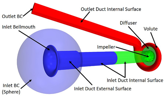
Figure 1.
Geometry of the CFD model.
The present study incorporates impeller rotation and all blade passages to capture the unsteady interaction of the impeller blades and asymmetric volute. In addition, the tip clearance region between the impeller blade tips and shroud is sufficiently resolved to capture tip leakage flow. Table 2 summarizes the detailed boundary conditions applied for each of the three fluid regions shown in Figure 1, along with their total cell count.
Table 2.
Computational domain cell count and boundary conditions.
The total cell count of the present model is 5.1 million (polyhedral cells with prism layers at the walls). The mesh is most refined in the vicinity of the impeller and diffuser, where the rotating region contains 3.95 million cells (approximately 77% of the total). Figure 2 shows an example of the mesh refinement within (and in front of) the impeller, including the blade leading edges. The increased number of faces for polyhedral cells allows for a lower cell count than that comprised of tetrahedral cells without sacrificing accuracy. Polyhedral cells also allow for a smoother transition of grid sizes (from walls to core), faster convergence, and improved gradient calculation due to the increased number of cell neighbors. In order to balance accuracy and runtime for these relatively long-duration, unsteady simulations, the near-wall prism layer height is specified to obtain a relatively high ) mesh. The ‘all-’ wall treatment in STAR-CCM+ is therefore adopted, where wall functions are used to model the viscous sublayer when the mesh resolution is inadequate. The global maximum cell size (within the compressor and ducting, excluding the spherical inlet portion) is limited to 1.44 mm, such that a minimum of 20 cells are utilized to resolve pressure fluctuations at a frequency of 12 kHz (wavelength of 28.83 mm at 298 K) [34]. This relatively coarse mesh is used within the up and downstream regions of the domain, which are further from the impeller. Within the rotating region, the mesh resolution is significantly finer (recall Figure 2). The minimum cell size on the surface of the impeller is about 30 μm, and the maximum cell size in the volume mesh surrounding the inducer region of the impeller is limited to 0.5 mm. Surface and volume mesh growth rates are limited to a factor of 1.2 in order to provide a gradual transition of cell size throughout the domain.
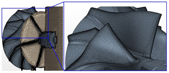
Figure 2.
Illustration of surface mesh on the impeller along with volume mesh on planes passing through the axis of rotation and the leading edge of main impeller blades.
The working fluid is standard air with constant material properties, and the compressible ideal gas model is employed. These fluid properties are listed in Table 3. At wall boundaries, the no-slip velocity and adiabatic thermal conditions are utilized. In this code, the finite volume method is used to transform the governing equations into a form that can be solved numerically, and the present study utilizes the coupled algebraic multi-grid (AMG) solver with a second-order spatial discretization scheme for the diffusive flux while Roe’s scheme is utilized for the inviscid flux. Both the coupled implicit and turbulence AMG solvers use the flex cycle to automatically optimize the relationship between the coarse and fine mesh cycles. A second-order implicit time-marching scheme is used with a number of sub-iterations at each time step to reduce the residuals by at least six orders of magnitude (for each time step). The unsteady Reynolds-Averaged Navier–Stokes (URANS) equations are solved, while the closure is provided by the shear stress transport (SST) k-ω turbulence model [35,36]. The time step for the present CFD predictions is 60 ns, such that the impeller rotates 0.0288° each step (12,500 time steps per revolution). This stringent time step was selected to maintain the global maximum convective Courant Number near unity. The simulations were considered converged when the fluctuations in the distribution of isentropic efficiency with respect to time reduced below 1%. The simulations were run for a total physical time of at least 40 ms (about 53 impeller revolutions).
Table 3.
Fluid (air) properties.
2.2. Model Assumptions
The assumptions in the present CFD modeling are summarized below:
- Working fluid (air) has constant material properties and obeys the ideal gas law.
- The fluid zones have adiabatic walls.
- All duct, impeller, shroud, diffuser, and volute walls are smooth.
- The ‘all-’ wall treatment with a wall mesh of around 30 is utilized.
- Turbocharger shaft vibrations and speed fluctuations are neglected.
- URANS (k-ω SST) turbulence model with a linear constitutive relation between Reynolds stress and strain rate is used.
3. Results and Discussion
3.1. Operating Points and Model Validation
3.1.1. CFD Operating Points
Three operating points were chosen for the CFD predictions as listed in Table 4.
Table 4.
CFD operating points.
The operating points were chosen such that the first point (77 g/s) is the maximum flow rate on the OSU turbocharger bench stand at a rotational speed of 80,000 rpm; 57 g/s is an operating point at the peak efficiency region, which is just above the flow rate threshold (55 g/s) when reversed flow was first observed experimentally in the inlet duct at this speed; and for the last operating point (30 g/s), the phenomenon of inlet recirculation is rather significant at the compressor inlet, where the reverse flow propagates upstream and subsequently becomes entrained back into the forward-moving fluid. Table 4 also lists the flow coefficient [7]
corresponding to each operating point, where is the actual mass flow rate, is the inlet air density, is the exducer tip speed, and is the impeller exit diameter. Also shown in Table 4 is the Reynolds Number
corresponding to each mass flow rate, where is the inlet duct diameter (=0.047 m), is the centerline mean axial velocity in the inlet duct at an axial location of 23.2 mm from the inducer plane, and is the dynamic viscosity.
3.1.2. Performance and Efficiency Comparison
Figure 3a shows the comparison of compressor characteristic predictions (at 80 krpm): total-to-total pressure ratio,
versus corrected mass flow rate,
from CFD (open symbols) with steady-state experimental data (closed symbols) from the turbocharger bench, where and are the total pressures at the compressor inlet and outlet, respectively, = 298 K is the reference temperature, and = 100 kPa is the reference pressure. Figure 3b illustrates the comparison of compressor total-to-total isentropic efficiency predictions from CFD to experimental data. The close agreement between the predictions and the experimental data demonstrates that the model is capable of accurately predicting compressor performance and efficiency.
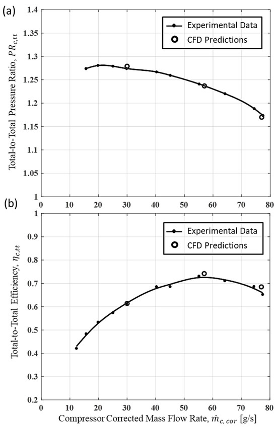
Figure 3.
(a) Comparison of compressor characteristic predictions at 80 krpm from CFD with steady-state experimental data, and (b) comparison of compressor isentropic efficiency predictions at 80 krpm from CFD with steady-state experimental data.
3.1.3. Velocity Field Comparisons between Predictions and Experiments
In this section, the flow field at the compressor inlet obtained from the CFD predictions is compared with experimental data obtained earlier using the Particle Image Velocimetry technique [28,29,30]. The comparisons are presented in terms of color contours as well as velocity profiles. These validations are provided for the operating points of 77 and 30 g/s. Since the flow field at 57 g/s in front of the impeller (within the PIV domain) is qualitatively very similar to that at 77 g/s, the comparisons for this mass flow rate have been excluded.
Figure 4a presents the comparison of time-averaged axial velocities on an axial plane passing through the center of the compressor wheel at 77 g/s. The upper portion (above the dot–dash centerline or axis of rotation) of the figure is from 3D CFD predictions, while the bottom half is obtained from PIV measurements. Similar comparisons at 30 g/s are provided in Figure 4b,c for mean axial and tangential velocities, respectively. The tangential velocities at the compressor inlet are negligible at 77 g/s and are not presented here. The velocities are presented in terms of color contours, where the Cartesian coordinate system utilized is illustrated in Figure 4a. The axial domain portrayed in Figure 4 corresponds to the PIV interrogation domain [30]. The horizontal axis (‘Axial Distance, ℓ [mm]’) of the figure denotes the axial distance from the compressor nut (or origin) along the negative X axis. The origin at ℓ = 0 mm is 12.7 mm from the leading edges of the main impeller blades. The center of the duct is at a radius of r = 0 mm, and |r| = 23.5 mm corresponds to the inner surface of the inlet duct walls. The regions in the PIV domain affected by laser light reflections from the compressor nut and blades are covered by a gray oval. The sign convention adopted for axial velocity (X velocity) is positive for flow entering the impeller (from right to left in Figure 4a,b) and negative for reverse flow. Tangential velocity (Z velocity) in Figure 4c is positive for flow moving into the plane under investigation. The rotation of the compressor is in the clockwise direction, that is, out of the plane of the page at the bottom and into the plane of the page at the top. This is depicted in Figure 4c by a black arrow around the centerline. Figure 4 illustrates good qualitative agreement between the predictions and measurements for both operating points.
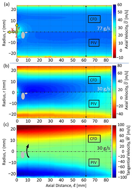
Figure 4.
Contour plots of time-averaged (a) axial velocity (at 77 g/s), (b) axial velocity (at 30 g/s), and (c) tangential velocity (at 30 g/s) on an axial plane passing through the axis of rotation from 3D CFD data above the center line and PIV data below.
For a more quantitative analysis, velocity profiles are presented next from CFD simulations and PIV measurements for two different configurations. Figure 5a presents the radial and tangential velocity profiles on a cross-sectional plane 2 mm in front of the main blade leading edges for a particular azimuthal orientation (illustrated through the schematic in Figure 5a). This configuration is first chosen because, being close to the impeller, the radial and tangential velocities at 77 g/s are non-zero (albeit small). The PIV data [29] are shown in circular symbols and CFD using triangles. At 77 g/s, the tangential and radial velocities are presented in blue and green, respectively, while the corresponding colors at 30 g/s are red and violet. The ordinate in these plots is the relative height, which is given as
where H is the total height from hub to shroud, h is the local height from the hub, R is the radius, (=4.97 mm) is the radius of the hub at the inducer plane, and (=19.95 mm) is the radius of the shroud at the inducer plane. Thus, h/H ranges from 0 at the hub to 0.977 in front of the blade tip. The available experimental data point closest to the hub corresponds to h/H = 0.07. Now, the experimental data corresponding to Figure 5a is obtained from 2D PIV experiments, where the out-of-plane component of velocity, that is, axial velocity, was not available. So, the axial velocity profiles are presented instead for a fixed location (ℓ = 10.5 mm) on the plane passing through the axis of rotation (Figure 5b). The experimental traces are shown in red, and the predictions are shown in blue. Solid lines are used for 77 g/s, and dashed lines for 30 g/s. The comparisons in Figure 5a,b show that while the CFD results agree fairly well with the experiments, the predicted peak velocity magnitudes at 30 g/s are slightly higher. This discrepancy between the measurements and the predictions may be because of a combination of increased uncertainty of the PIV data near the walls due to reflections and glare and the inaccuracies in the CFD model for endwall flows. Since the current predictions do reasonably capture all the trends shown by the experimental data, they are used next to further examine different characteristics of the flow field.
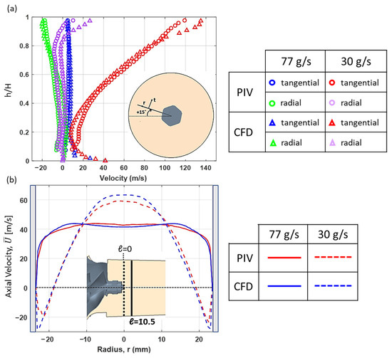
Figure 5.
(a) Comparison of time-averaged radial and tangential velocity profiles on a cross-sectional plane at ℓ = −10.7 mm (2 mm in front of the main blade leading edges) between experiments [PIV (circles)] and predictions [CFD (triangles)]; (b) comparison of time-averaged axial velocity profiles at a fixed axial location (ℓ = 10.5 mm) on an axial plane passing through the center of the compressor wheel for PIV (red) and CFD (blue).
3.2. Flow Field Analysis
This section illustrates the flow field inside the impeller with a focus on the generation of both stationary (Section 3.2.1) and rotating stall cells (Section 3.2.2).
For analyzing compressor stall in Section 3.2.1 and Section 3.2.2, eight different cross-sectional planes at specific distances from the leading edge of the main impeller blades are chosen. These planes (labeled from a to h) and their respective distances with respect to the leading edges of the main blades are shown in Figure 6. The first plane (labeled a) is 2 mm in front of the leading edges, which is the same as the plane for the 2D PIV investigation domain (recall Figure 5a). The second plane (b) is the inducer plane. The other planes are within the impeller at successively larger distances from the leading edge. Plane e, which is 8.78 mm from the main blade’s leading edges, is just in front of the leading edges of the splitter blades. It is also the location from where the shroud’s axial to radial bend starts becoming prominent. Plane h passes through the exducer and the diffuser.
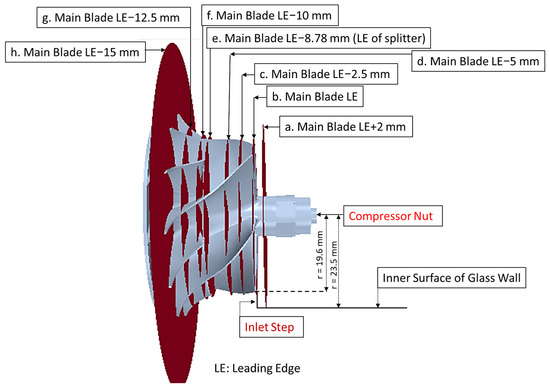
Figure 6.
Eight cross-sectional planes with respect to the impeller for flow field analyses.
3.2.1. Analysis of Stationary Stall Cells
While Figure 4 shows how the relatively simple flow moving axially into the compressor at 77 g/s (Figure 4a) changed into a swirling three-dimensional flow field at 30 g/s (Figure 4b,c) with an annular region of negative axial velocity near the periphery (reversed flow), the present section analyzes from where this reverse flow is generated and its relationship with stationary stall cells. The results are presented mainly at the lowest flow rate of 30 g/s since the phenomenon of reversed flow was observed to be most prominent here (out of the three operating points). First, the axial velocity distribution within the impeller at 30 g/s is presented in Figure 7. The contours labeled from a to h correspond to the same planes shown in Figure 6. The individual sizes of the color contours representing these planes preserve the ratios of their cross-sectional areas except for contour ‘h’, which had to be scaled down further so that it could be contained in the same figure. The splitter blades in contours ‘g’ and ‘h’ have been shaded in gray. The black lines in Figure 7 denote the iso-lines for zero mean axial velocity.
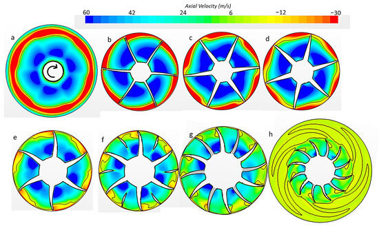
Figure 7.
Instantaneous axial velocity contours on different cross-sectional planes (a–h) within the impeller at 30 g/s.
The color convention here is consistent with that of Figure 4, where negative axial velocity (shades of yellow and red) indicates reverse flow coming out of the compressor toward the inlet. Recalling Figure 4b, it is evident that at this operating point, the phenomenon of inlet recirculation has been established within the inlet duct, and Figure 7a shows the reverse flow occupying an annular region near the periphery. On the inducer plane, reverse flow is present near the blade tips (Figure 7b), but it occupies a larger area near the pressure surface than the suction surface. Figure 7c,d show that as the reverse flow makes its way out of the impeller progressively through planes d, c, and b, there is a gradual increase near the pressure surface blade tips in the thickness of the annular region of negative axial velocity. On the other hand, further inside the impeller, on planes e and f, the reverse flow is more or less confined near the blade tips between the suction surface of the main blades and the pressure surface of the splitter blades with the thickness of the reverse flow region being slightly more skewed toward the main blades. On plane g, the magnitude of the reverse flow has substantially decreased, and on a time-averaged basis, only pockets of negative axial velocity are observed near the shroud at the suction and pressure surfaces of the main and splitter blades, respectively (Figure 7g). The vector plot of relative velocity on plane f at 30 g/s is shown in Figure 8, which clearly shows that the portion of the blade passage near the shroud between the suction surface of the main blades and the pressure surface of the splitter blades is stalled (axial velocity is nearly zero). The stall cells in Figure 8 are identified using red dashed ovals. Similar structures are also observed on planes e and g between the suction and pressure surfaces of the main and splitter blades, respectively. While these stall cells were also observed at 57 g/s, they have grown in size and have become more prominent at this operating point. On the other hand, these were not observed at all at 77 g/s. The following discussion will help with further characterization of these stall cells and illustrate the physics behind their generation and location with respect to the blades.
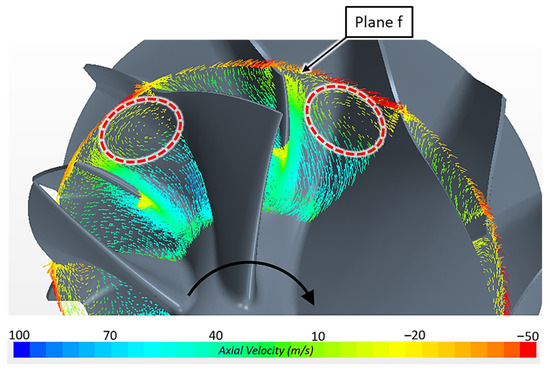
Figure 8.
Frontal view of the impeller showing vector plot of relative velocities on plane f at 30 g/s.
Figure 9a presents the mean axial velocity (above the centerline) and mean absolute pressure (below the centerline) on an axial plane passing through the axis of rotation. The solid black lines denote the iso-lines for zero mean axial velocity, and the three dashed vertical lines denote the axial locations of planes e, f, and g (recall Figure 6). As the compressor mass flow rate is reduced from 77 to 57 and then to 30 g/s, the incidence angle at the blade tips increases, and flow separates from the blade suction surface [2,28]. A strong adverse pressure gradient is observed within the impeller (Figure 9a), which pushes this separated fluid toward the inlet, thus helping in the generation of reverse flow. Note that the thickness of the reverse flow region near the shroud increases sharply around plane e as compared to further within the impeller, which is also the location where the axial to radial bend of the shroud starts. Figure 9b,c present the radial velocity distribution and the relative velocity vector plot, respectively, on the same plane. The right boundary of Figure 9c is identified on the top half of Figure 9a using a dashed white line. Figure 9c shows that a considerable portion of the forward flow is unable to follow the impeller’s axial to radial bend against the adverse pressure gradient and becomes entrained by the reverse flow and the tip leakage flow moving back out of the impeller. This further strengthens the reverse flow at this operating point and also explains the sudden increase in the annular thickness of the reverse flow region inside the impeller as observed in Figure 9a. Upstream of plane e, the axial velocity magnitude is high, while the radial velocity starts increasing downstream of plane g. The black oval in Figure 9c indicates a low-momentum region near the shroud between planes e and g that is conducive to the generation of stationary stall cells. Note that even on a highly saturated color scale, the axial velocity within the oval region is close to zero. It identifies the axial location within the compressor where the stall cells are generated. Thus, the stall cells observed in Figure 8 are axially located in the wake of the blockage created by the annular reverse flow region formed near the shroud of the impeller, where the axial to radial bend of the shroud is prominent.
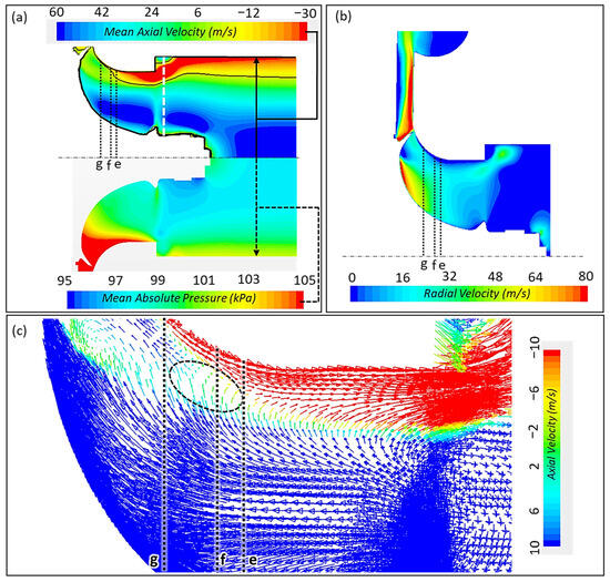
Figure 9.
At 30 g/s: (a) distributions of mean axial velocity (above the centerline) and mean absolute pressure (below the centerline); (b) distribution of radial velocity; (c) relative velocity vector plot on an axial plane passing through the center of the wheel.
Figure 10a shows the contour plot of relative total pressure on plane f (same plane as in Figure 8) at 30 g/s. The regions where stall cells were observed in Figure 8 between the suction surface of the main blades and the pressure surface of the splitter blades also correspond to zones of low relative total pressure. This is further illustrated in Figure 10b, where the same contour plot of relative total pressure is shown within one blade passage, and the relative velocity vectors are portrayed in the adjacent one. The vectors’ color bar representing axial velocity has a different color scheme from that of Figure 8 to improve the contrast with the relative total pressure contour. The figure clearly illustrates the non-uniformities in the distribution of relative total pressure on plane f. It can be shown theoretically that gradients in relative total pressure distributions can lead to the generation of secondary flows within the impeller [8,37]. The impact of the generation of secondary flows can be broadly classified under the effects of rotation and curvature. The effect of rotation [Coriolis force (−2ρ × ), where and are angular velocity and relative velocity vectors, respectively] starts to become potent as the flow is turned in the radial direction and is most effective near the outlet. For example, for an impeller rotating in the clockwise direction, the core flow experiences Coriolis force from suction to the pressure surface of the blades, which is, in turn, balanced by pressure gradients acting in the opposite direction. For a region of low-momentum fluid (for example, within the boundary layer in an adverse pressure gradient), the relative velocity and hence the magnitude of Coriolis force acting on it is low, and the pressure gradients (same magnitude as for core flow) tend to force this low-momentum fluid toward the suction surface. Similarly, as the core flow moves along the axial to radial bend of the shroud, the centrifugal forces are balanced by pressure gradients. But, if a low-momentum region (or a region of low relative stagnation pressure) is formed due to some reason, the pressure gradients will try to force that fluid toward the shroud. This may partially explain why the stall cells in Figure 8 were located near the shroud beside the suction surface of the main impeller blades.
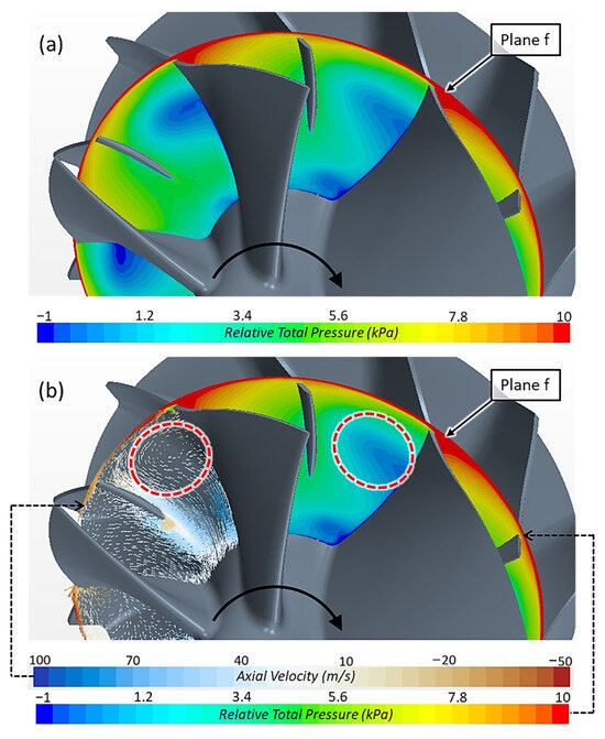
Figure 10.
Frontal view of the impeller at 30 g/s showing on plane f (a) contour plot of relative total pressure (b) relative total pressure contour in one blade passage and relative velocity vectors in the adjacent one colored by axial velocity.
Japikse [8] highlighted the role of a centrifugal impeller passage in diffusing the high kinetic energy of the incoming flow to maximize the performance, while failure to do so results in a penalty in terms of efficiency. As these stall cells occupy a large portion of the blade passage near the shroud, they reduce the effective blade passage height and, hence, the net diffusion of the relative flow. Furthermore, as these stall cells increase the non-uniformity in the flow field (for example, exacerbate the jet–wake structure at the impeller exit), they also lead to further flow losses within the compressor. This phenomenon of a part of the blade passage being stalled between planes e and g was first observed at 57 g/s, which is very close to the peak efficiency regime of the compressor (recall Figure 3b). Now, as the mass flow rate is further reduced to 30 g/s, these stall cells grow stronger, and the compressor efficiency is also observed to decrease quite rapidly (Figure 3b).
While the stall cells, as observed in Figure 8, are present to a lesser extent at 57 g/s, they are completely absent at 77 g/s. The adverse pressure gradient within the impeller is far less severe at 77 g/s than in Figure 9a, and because of the increased mass flow rate, the forward flow momentum is higher, resulting in the absence of any significant reverse flow within the impeller. Unlike Figure 9c, a low-momentum region is not observed on planes e, f, and g, and thus no stall cells are formed. At 57 g/s, while the reverse flow is not strong enough to penetrate back into the inlet duct, there is still local recirculation within the impeller, and the flow field between planes e and g is similar to that at 30 g/s (recall Figure 9c).
3.2.2. Analysis of Rotating Stalls
The analysis here focuses on the operating point at 57 g/s, the mass flow rate where the phenomenon of inducer rotating stall was observed to be most dominant. Figure 11 presents the dynamic pressure fluctuation on planes a–h (recall Figure 6) at 57 g/s. Alternate cells of positive and negative pressures are visible near the blade tips and are most prominent on plane b (inducer plane). While they are still visible on planes c and d, they appear to become less distinct further inside the impeller.
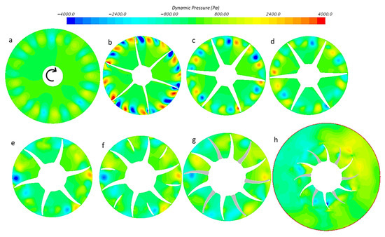
Figure 11.
Dynamic pressure contours on different cross-sectional planes (a−h) within the impeller at 57 g/s.
A time-resolved animation (created in the laboratory frame of reference) from the present URANS simulation at 57 g/s portraying how these stall cells on the inducer plane rotate with respect to the compressor wheel is available online [38]. In the animation (or Figure 11b), a total number of 13 cells were found to rotate in the same direction as that of the impeller at about 45% of the impeller blade speed. These were observed to a lesser extent at 77 g/s on planes c and d and are hardly present at 30 g/s (see Appendix B).
Figure 12a presents the frequency domain analysis of a virtual pressure probe in front of the blade tips (radial location of 19.6 mm) and 1 mm in front of the inducer plane at 57 g/s, and Figure 12b shows a comparison of the sound pressure level (SPL) distribution versus frequency at the chosen three flow rates. The rotor order is also presented as an alternate X-axis (in green) in both Figure 12a,b. A rotor order of 1 corresponds to the synchronous frequency of 1.33 kHz and 6 to the blade passing frequency of 8 kHz, respectively. For an impeller with Z main blades operating at a rotational speed of N rpm, the blade passing frequency () can be computed as
similarly, the frequency corresponding to the rotating stall cells (RS) is
where is the rotational speed of the cells in rpm, and is the number of rotating stall cells; the frequency of interaction of the RS cells with the rotor or impeller blades () [39,40,41] is
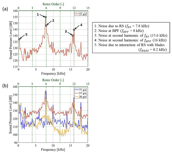
Figure 12.
From a virtual pressure probe at a radial location of 19.6 mm and an axial location of 1 mm in front of the inducer plane: (a) predicted sound pressure level versus frequency (or rotor order) at 57 g/s; (b) comparison of predicted SPL versus frequency (or rotor order) at 77 (blue), 57 (orange), and 30 g/s (yellow).
In the present case with N = 80 krpm and Z = 6, , , and , computed using Equations (6)–(8) are 8, 7.8, and 0.2 kHz, respectively. Figure 12a identifies the noise generated at , , their corresponding second harmonics, and also using black circles and arrows (labeled 1 through 5). At 57 g/s, where the RS cells were found to be most dominant among the three mass flow rates, the SPL corresponding to is even higher than that at . The average sound pressure level over the entire frequency range of 0 to 20 kHz is also highest at 57 g/s among the three flow rates (Figure 12b). Pressure probes at the same cross-sectional plane situated at other azimuthal locations in front of the blade tips were also found to show very similar trends.
Figure 13a allows the visualization of the tip leakage flow using relative velocity streamlines at 57 g/s. The dashed black lines show the locations of the seeding points from which the streamlines are generated. These seeding points were distributed following the profiles of the main blade tip surfaces, starting from the inducer all the way to the exducer. Radially, these seeding points are located midway between the blade tip surface and the shroud, that is, in the middle of the tip clearance region, while following the main blade tip surface curvature. Thus, the streamlines generated from these seed points should follow the tip leakage flow. These streamlines in Figure 13a are colored using axial velocity, where positive values indicate forward flow into the impeller and negative values illustrate flow directed out of the impeller toward the inlet duct (consistent with the convention of Figure 4). Figure 13a shows that at 57 g/s, although the streamlines originating near the inducer tend to initially move back toward the inlet (corresponding to red colors) and do spill over the leading edges, they do not move out much further beyond the inducer plane and become entrained back into the impeller due to the shear caused by the forward moving core flow. This interaction of the tip leakage flow with the incoming core flow results in a wavy shear layer at the inducer plane (Figure 13b), and the associated Kelvin–Helmholtz instability is possibly a major reason behind the unsteadiness and pressure fluctuations observed on the same plane. This interaction also gives rise to several vortical structures near the blade tips, which are identified in Figure 13c (marked by red dashed circles/ovals) using iso-surfaces of criterion [42,43], a popular vortex identification technique. Many of these structures also protrude beyond the inducer plane. Figure 13b shows that the reverse flow forms distinct pockets around the circumference near the blade tips. A total of 13 such pockets are observed, which is consistent with the number of stall cells noted earlier in Figure 11b (number of red/blue blobs) or the number of vortical structures identified in Figure 13c.
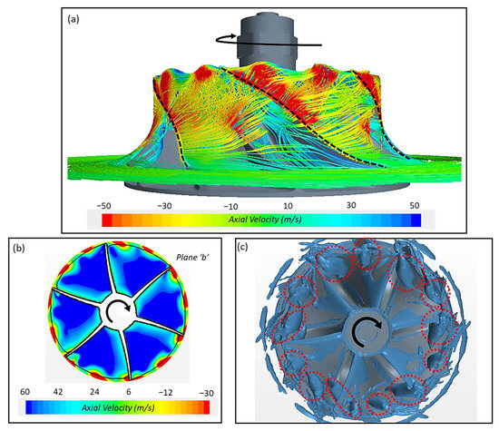
Figure 13.
At 57 g/s: (a) streamlines illustrating tip leakage flow; (b) distribution of instantaneous axial velocity on plane b; (c) iso-surfaces of criterion for an iso-contour threshold of = −8 × 10⁸.
While the shear layer shown in Figure 13b generates circumferential (tangential) vorticity, the region near the blade tips on plane b is characterized by elevated magnitudes of all three vorticity components (illustrated in Figure 14), including radial vorticity, which can aid the circumferential propagation of the stall cells. Note that all the streamlines in Figure 13a eventually turn in the meridional direction and move out through the exducer. At 77 g/s, unlike Figure 13a, spillage of tip leakage flow beyond the main blade leading edges is not observed (Figure 15a). This is because the adverse pressure gradient within the impeller at 77 g/s is less than that at 57 g/s, and the streamlines for the tip leakage flow become entrained well within the impeller without creating a wavy pattern on the inducer plane, as observed in Figure 13a. The corresponding interaction creates dynamic pressure fluctuations at 77 g/s on planes c and d, albeit to a lesser extent than 57 g/s (see Appendix B). On the other hand, at 30 g/s, the adverse pressure gradient is much stronger, and the tip leakage flow smoothly moves out of the impeller back into the inlet duct without becoming entrained by the forward flow near the inducer plane (Figure 15b). Thus, rotating stall cells are not observed at the inducer or further within the impeller at 30 g/s. Also note that while the rotating stall is the strongest at 57 g/s, the compressor efficiency at 57 g/s is much higher than at 30 g/s. Thus, the effect of the inducer rotating stall on compressor isentropic efficiency may not be highly significant in this case.
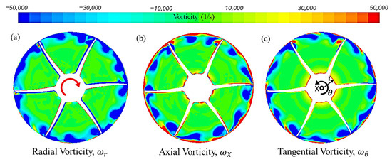
Figure 14.
At 57 g/s and plane b: distributions of (a) radial, (b) axial, and (c) tangential vorticity.
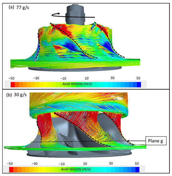
Figure 15.
Streamlines illustrating tip leakage flow at (a) 77 g/s and (b) 30 g/s.
In conclusion, the rotating stall was generated due to the interaction of the tip leakage flow with the incoming core flow and the associated shear layer instability. It was observed first within the impeller at the highest flow rate of 77 g/s on planes c and d (2.5 and 5 mm from the inducer, respectively). The phenomenon grew stronger with a reduction in flow rate and was the strongest on the inducer plane at 57 g/s, a mass flow rate that is just above the threshold where the tip leakage flow is able to leave the impeller through the inlet and create a stream of reversed flow. As the reversed flow is generated with a further decrease in mass flow rate, the tip leakage flow is no longer entrained back into the impeller at the inducer by the core forward moving fluid, and due to this lack of interaction (entrainment of tip leakage flow), inducer rotating stall is no longer observed. This observation of the inducer rotating stall for a turbocharger compressor being strongest near the peak efficiency region is unique from the literature perspective.
4. Conclusions
The salient features of this work are summarized as follows:
- Three-dimensional CFD predictions were carried out to study the turbocharger compressor flow field at three discrete mass flow rates of 77, 57, and 30 g/s at a fixed rotational speed of 80,000 rpm. The three operating points are chosen such that 77 g/s is the maximum mass flow rate at 80 krpm without any flow reversal; 57 g/s is the operating point near peak efficiency where the reverse flow from the impeller does not yet reach the inlet duct walls; and the last operating point, 30 g/s, is a flow rate where the inlet recirculation is well established within the inlet duct. The predictions agreed well with measurements from the turbocharger stand, including compressor performance and efficiency. The velocity distributions from the CFD predictions were also validated against PIV measurements obtained earlier.
- The simulations were thereafter used to analyze the compressor flow field with a focus on the stall instability. The study identified the parts of the turbocharger compressor map where stationary and inducer rotating stall phenomena are observed. While stationary stall cells started forming within the impeller near the peak efficiency point at 57 g/s, they became more pronounced with further reduction in flow rate and were not observed at all at the maximum flow condition (77 g/s). On the other hand, the inducer rotating stall was found even at the maximum flow rate of 77 g/s, which became most prominent near the peak efficiency point (at 57 g/s) and disappeared at lower flow rates.
- The present work also identifies the locations within the impeller where the stationary stall cells develop. These stall cells were identified near the shroud exclusively between the suction surface of the main blades and the pressure surface of the splitter blades. Axially, these were located between 8.78 mm and 12.5 mm from the leading edges of the main blades, a region where the axial to radial bend of the shroud starts to become prominent. With a reduction in the compressor mass flow rate from 77 to 57 and then to 30 g/s, the incidence angle at the blade tips increases, and flow separation takes place from the suction surface of the main blades. The strong adverse pressure gradient inside the impeller pushes this separated fluid back toward the inlet, leading to the generation of the reverse flow. A part of the core flow within the impeller cannot follow the axial to radial bend of the shroud against this adverse pressure gradient and becomes entrained back toward the inlet by the reverse flow and the tip leakage flow. This creates a region of low-momentum fluid in the wake of the blockage created by the strong annular reverse flow pattern, giving rise to the stall cells. These cells also correspond to regions of low relative total pressure. The non-uniformities or gradients in the distributions of relative total pressure indicate a possible role of secondary flows in the generation and orientation of the stationary stall cells.
- The stationary stall cells occupy a significant portion of the blade passage at 30 g/s, thereby reducing the effective blade height and the diffusion of the relative flow. They increase the non-uniformities in the flow field, leading to further flow losses. These effects are reflected in the deterioration of compressor efficiency at this operating point.
- The study further revealed the presence of rotating stall cells near the blade tips on the inducer plane at 57 g/s. These manifested as alternating cells of positive and negative dynamic pressure, which rotated in the same direction as that of the compressor wheel at about 45% of the inducer tip speed. These were generated mainly due to the entrainment of the tip leakage flow by the forward-moving core flow, giving rise to a wavy, unstable shear layer at the inducer plane along with several vortical structures near the blade tips. These instabilities were observed to a lesser extent within the impeller at 77 g/s, about 2.5 to 5 mm from the inducer plane, and were almost completely absent at 30 g/s. The prominence of the inducer rotating stall at somewhat higher flow rates is relatively rare, and the present paper illustrates the mechanism that led to its formation and subsequent disappearance at lower flow rates.
- The study also characterized how the entropy generation (associated irreversibilities) within the compressor changes at the three flow rates. The entropy generation was mainly caused by viscous dissipation and increased in strength with a reduction in compressor mass flow rate. At 77 g/s, it was found to mainly occur within the impeller near the shroud, with the core flow appearing to be almost isentropic. On the other hand, at 30 g/s, the entire compressor blade passage showed significant entropy generation, with the peak still being near the shroud. Irreversibilities were also found to occur in the inlet duct at 30 g/s within the annular reverse flow region and in the shear layer between the reverse and forward flows. The interaction of the tip leakage flow with the blades and core flow, along with the production of reverse flow, are major sources of entropy generation within the compressor.
Author Contributions
Conceptualization, D.K.B.; methodology, D.K.B.; software, D.K.B. and P.S.; validation, D.K.B.; formal analysis, D.K.B.; investigation, D.K.B.; resources, A.S.; data curation, D.K.B.; writing—original draft preparation, D.K.B.; writing—review and editing, D.K.B., A.S. and P.S.; visualization, D.K.B. and P.S.; supervision, A.S.; project administration, A.S.; funding acquisition, A.S. All authors have read and agreed to the published version of the manuscript.
Funding
This research received no external funding.
Data Availability Statement
The raw data supporting the conclusions of this article will be made available by the authors on request.
Conflicts of Interest
The authors declare no conflicts of interest.
Nomenclature
| b | Exducer b-width |
| D | Diameter |
| f | Frequency |
| h | Local blade height from hub |
| H | Total height from hub to shroud |
| k | Turbulent kinetic energy; thermal conductivity |
| ℓ | Upstream distance from origin along negative X-axis |
| m | Number of rotating stall cells |
| Mass flow rate | |
| N | Rotational speed in rpm |
| p | Pressure |
| Pr | Prandtl number |
| PR | Pressure ratio |
| r, R | Radius |
| RS | Rotating stall |
| Rotor-rotating stall | |
| Mean strain rate tensor | |
| Fluctuating strain rate | |
| Volumetric rate of entropy generation | |
| Temperature | |
| Mean static temperature | |
| Fluctuating static temperature field | |
| Centerline mean axial velocity in the inlet duct | |
| Exducer tip speed | |
| w | Relative velocity |
| X | Axial direction |
| Y | Radial direction |
| Z | Out-of-plane (tangential) direction; number of main blades |
| Greek Symbols | |
| Thermal diffusivity | |
| Dissipation rate | |
| Compressor isentropic efficiency | |
| Dynamic viscosity | |
| Density | |
| Flow coefficient | |
| Angular velocity; vorticity; specific dissipation rate | |
| Subscripts | |
| 0 | Total (stagnation) |
| 1 | Compressor inlet location |
| 2 | Compressor outlet location |
| BPF | Blade passing frequency |
| c | Compressor |
| cor | Corrected quantity |
| h | Hub of impeller |
| ref | Reference quantity |
| s | Shroud of impeller |
| t | Turbulent |
| therm | Thermal |
| tip | Tip of inducer |
| tt | Total-to-total |
| visc | Viscous |
| X | Axial direction |
| Y | Radial direction |
| Z | Tangential direction |
| θ | Tangential component |
Appendix A. Analysis of Entropy Generation at the Compressor Inlet
This appendix provides a brief discussion of how the irreversibilities at the compressor inlet vary with respect to flow rate. Since the flow field of a centrifugal compressor is rather complex with a variety of interacting phenomena like boundary layer separation and inlet recirculation, secondary flow development due to effects of rotation and blade curvature, tip leakage flow, and possible shock waves, Denton [44] acknowledged that it is difficult to distinguish the different sources of losses in a centrifugal compressor (for example, blade boundary layer loss, endwall loss, tip leakage loss), and thus quantifying the entropy generation is a popular approach that provides a quantitative estimate of the net loss [44]. While analyzing the efficiency of any thermal system, it is also important to account for the second law of thermodynamics as reduced entropy generation implies increased available work or exergy, and hence a possibility for a more efficient system design [45,46].
In the absence of shock waves within the impeller, the volumetric rate of entropy generation () mainly has two components—a thermal component () which arises due to heat transfer under a finite temperature difference, and the second is due to viscous dissipation () [47,48]:
where
and
The first terms in Equations (A2) and (A3) represent the contributions from the mean flow variables, where denotes the mean static temperature and denotes the mean strain rate, and the second terms represent the contributions from the fluctuating variables with and denoting the fluctuating temperature field and the fluctuating rate of strain, respectively. The variables and denote thermal conductivity and dynamic viscosity, respectively. Since the RANS turbulence model is not ideally suited for exactly determining the terms based on the fluctuating components [second terms in Equations (A2) and (A3)], Kock and Herwig [45] outlined a procedure for modeling these quantities in terms of the mean flow variables, and thus, Equations (A2) and (A3) can be reformulated as
where is turbulent thermal diffusivity and is the molecular thermal diffusivity, and
where is the turbulent dissipation rate and is the density.
In the present work, was evaluated by multiplying the specific dissipation rate with the turbulent kinetic energy and was evaluated using the eddy viscosity available from the RANS model, along with the assumption of the turbulent Prandtl number equal to 0.9. Figure A1a–c show contours of [recall Equation (A1)] evaluated using Equations (A4) and (A5) on an axial plane passing through the center of the impeller at 77, 57, and 30 g/s, respectively. The origin (X = 0, Y = 0) for these plots is at the tip of the compressor nut, and ℓ > 0 corresponds to the PIV investigation domain consistent with, for example, Figure 4.

Figure A1.
Entropy generation on an axial plane passing through the axis of rotation of the impeller at (a) 77 g/s, (b) 57 g/s, and (c) 30 g/s.
Figure A1.
Entropy generation on an axial plane passing through the axis of rotation of the impeller at (a) 77 g/s, (b) 57 g/s, and (c) 30 g/s.

The present analysis determined that was more than two orders of magnitude smaller than , and so the distributions of are almost identical to those of . Figure A1a shows that at 77 g/s, the entropy generation is highest near the shroud in the blade passage within the impeller, mostly due to the shear between the tip leakage flow and the forward core flow. While there is also some entropy generation near the hub surface, is almost negligible for the core flow within the blade passage or upstream in the inlet duct. At 57 g/s, while the qualitative distribution of remains similar to that at 77 g/s, the zone with elevated entropy generation within the blade passage penetrates to lower spans from the shroud in Figure A1b as compared to Figure A1a. This is due to the generation of a recirculation region near the shroud between the annular reverse flow, which does not yet reach the inlet duct, and the forward-moving core flow. Also, note that while the region of high near the shroud at 77 g/s is entirely within the blade passage, at 57 g/s, it slightly extends beyond the inducer plane (ℓ = 12.7 mm, also the location of the inlet step) but does not yet reach the outer glass wall. This is because, at 57 g/s, the tip leakage flow spills over the blade leading edges trying to move out of the inducer plane and becomes entrained back into the impeller by the forward flow, giving rise to a wavy shear layer (recall Figure 13a,b) with vortical structures that slightly protrude beyond the tips of the blade leading edges (recall Figure 13c). At 30 g/s, the entire blade passage within the impeller shows strong entropy generation, with the peak still being near the shroud, where the tip leakage flow and the reverse flow are concentrated (recall Figure 9). As the reverse flow moves out into the inlet duct, there is considerable entropy generation near the periphery of the duct within the reverse flow region and the shear layer between the reverse and forward flow. For the core flow near the center of the duct, is still comparatively low. If the mass flow rate is reduced below 30 g/s, with the further strengthening of the annular flow reversal, this region of low in the core flow is expected to shrink further with increasing entropy generation within the compressor, as well as the inlet duct. The present analyses suggest that the tip leakage flow, its interaction with the blades and the core forward flow, and the generation of reverse flow within the impeller are major sources of irreversibilities. Thus, there may be scope for further improvements in impeller design, including optimizations of the blade curvature, axial to radial bend of the hub and shroud, inducer blade angle distribution, and tip clearance gap, which can not only reduce the irreversibilities but also improve compressor performance and isentropic efficiency.
Appendix B. Dynamic Pressure Analyses
Figure A2 and Figure A3 present the dynamic pressure fluctuation on planes a–h (recall Figure 6) at 77 g/s and 30 g/s, respectively. As compared to Figure 11, stall cells are observed at 77 g/s on planes c and d, whereas they are absent at 30 g/s.

Figure A2.
Dynamic pressure contours on different cross-sectional planes (a–h) within the impeller at 77 g/s.
Figure A2.
Dynamic pressure contours on different cross-sectional planes (a–h) within the impeller at 77 g/s.


Figure A3.
Dynamic pressure contours on different cross-sectional planes (a–h) within the impeller at 30 g/s.
Figure A3.
Dynamic pressure contours on different cross-sectional planes (a–h) within the impeller at 30 g/s.

References
- Heywood, J.B. Internal Combustion Engine Fundamentals; McGraw-Hill Inc.: New York, NY, USA, 1988. [Google Scholar]
- Baines, N.C. Fundamentals of Turbocharging; Concepts ETI: White River Junction, VT, USA, 2005. [Google Scholar]
- Dehner, R.; Selamet, A.; Keller, P.; Becker, M. Simulation of Deep Surge in a Turbocharger Compression System. In Proceedings of the ASME Turbo Expo, Copenhagen, Denmark, 11–15 June 2012; ASME Technical Paper GT2012-69124. American Society of Mechanical Engineers (ASME): New York, NY, USA, 2012. [Google Scholar]
- Dehner, R.; Selamet, A.; Keller, P.; Becker, M. Prediction of Surge in a Turbocharger Compression System vs. Measurements. SAE Int. J. Engines 2011, 4, 2181–2192. [Google Scholar] [CrossRef]
- Eckardt, D. Flow field analysis of radial and backswept centrifugal compressor impellers, Part 1: Flow measurement using a laser velocimeter. In Proceedings of the 25th ASME Annual International Gas Turbine Conference and Exhibit and 22nd Annual Fluids Engineering Conference, New Orleans, LA, USA, 9–13 March 1980. [Google Scholar]
- Krain, H. Swirling impeller flow. In Proceedings of the 32nd ASME Gas Turbine Conference and Exhibit, Anaheim, CA, USA, 31 May–4 June 1987; ASME Technical Paper 85-GT-85. American Society of Mechanical Engineers (ASME): New York, NY, USA, 1987. [Google Scholar]
- Cumpsty, N.A. Compressor Aerodynamics; Krieger: Malabar, FL, USA, 1989. [Google Scholar]
- Japikse, D. Centrifugal Compressor Design and Performance; Concepts ETI: White River Junction, VT, USA, 1996. [Google Scholar]
- Day, I.J. Stall, Surge, and 75 Years of Research. ASME J. Turbomach. 2016, 138, 011001. [Google Scholar] [CrossRef]
- Day, I.J.; Cumpsty, N.A. The Measurement and Interpretation of Flow Within Rotating Stall Cells in Axial Com pressors. J. Mech. Eng. Sci. 1978, 20, 101–115. [Google Scholar] [CrossRef]
- Day, I.J. Stall Inception in Axial Flow Compressors. ASME J. Turbomach. 1993, 115, 1–9. [Google Scholar] [CrossRef]
- Vo, H.D.; Tan, C.S.; Greitzer, E.M. Criteria for Spike Initiated Rotating Stall. ASME J. Turbomach. 2008, 130, 011023. [Google Scholar] [CrossRef]
- Camp, T.R.; Day, I.J. A Study of Spike and Modal Stall Phenomena in a Low-Speed Axial Compressor. ASME J. Turbomach. 1998, 120, 393–401. [Google Scholar] [CrossRef]
- Spakovszky, Z.S.; Roduner, C.H. Spike and Modal Stall Inception in an Advanced Turbocharger Centrifugal Compressor. ASME J. Turbomach. 2009, 131, 031012. [Google Scholar] [CrossRef]
- Mailach, R.; Lehmann, I.; Vogeler, K. Rotating Instabilities in an Axial Compressor Originating From the Fluctuating Blade Tip Vortex. ASME J. Turbomach. 2001, 123, 453–460. [Google Scholar] [CrossRef]
- März, J.; Hah, C.; Neise, W. An Experimental and Numerical Investigation into the Mechanisms of Rotating Instability. ASME J. Turbomach. 2002, 124, 367–374. [Google Scholar] [CrossRef]
- Pardowitz, B.; Moreau, A.; Tapken, U.; Enghardt, L. Experimental identification of rotating instability of an axial fan with shrouded rotor. Proc. IInst. Mech. Eng. Part A J Power Energy 2015, 229, 520–528. [Google Scholar] [CrossRef]
- Wu, Y.; Li, T.; Lai, S.; Tian, J.; Ouyang, H. Investigation of rotating instability characteristics in an axial compressor with different tip clearances. Proc. Inst. Mech. Eng. Part G J. Aerosp. Eng. 2021, 235, 2225–2239. [Google Scholar] [CrossRef]
- Grondin, J.; Trébinjac, I.; Rochuon, N. Rotating Instabilities Versus Rotating Stall in a High-Speed Centrifugal Compressor. In Proceedings of the ASME Turbo Expo, Oslo, Norway, 11–15 June 2018; ASME Technical Paper GT2018-76916. American Society of Mechanical Engineers (ASME): New York, NY, USA, 2018. [Google Scholar]
- Iwaraki, K.; Furukawa, M.; Ibaraki, S.; Tomita, I. Unsteady and Three-Dimensional Flow Phenomena in a Transonic Centrifugal Compressor Impeller at Rotating Stall. In Proceedings of the ASME Turbo Expo: Power for Land, Sea, and Air, Orlando, FL, USA, 8–12 June 2009; ASME Technical Paper GT2009-59516. American Society of Mechanical Engineers (ASME): New York, NY, USA, 2009; pp. 1611–1622. [Google Scholar]
- Tomita, I.; Ibaraki, S.; Furukawa, M.; Yamada, K. The Effect of Tip Leakage Vortex for Operating Range Enhancement of Centrifugal Compressor. ASME J. Turbomach. 2013, 138, 051020. [Google Scholar] [CrossRef]
- Cao, T.; Kanzaka, T.; Xu, L.; Brandvik, T. Tip Leakage Flow Instability in a Centrifugal Compressor. In Proceedings of the ASME Turbo Expo, Phoenix, AZ, USA, 17–21 June 2019; ASME Technical Paper GT2019-90217. American Society of Mechanical Engineers (ASME): New York, NY, USA, 2019. [Google Scholar]
- Guleren, K.; Turan, A.; Pinarbasi, A. Large Eddy Simulation of the Flow in a Low-Speed Centrifugal Compressor. Int. J. Numer. Methods Fluids 2008, 56, 1271–1280. [Google Scholar] [CrossRef]
- Miura, T.; Yamashita, H.; Takeuchi, R.; Sakai, N. Numerical and Experimental Study on Rotating Stall in Industrial Compressor. ASME J. Turbomach. 2021, 143, 081008. [Google Scholar] [CrossRef]
- Margot, X.; Gil, A.; Tiseira, A.; Lang, R. Combination of CFD and Experimental Techniques to Investigate the Flow in Centrifugal Compressors Near the Surge Line; SAE Technical Paper 2008-01-0300; SAE International: Warrendale PA, USA, 2008. [Google Scholar] [CrossRef]
- Hellstrom, F.; Gutmark, E.; Fuchs, L. Large Eddy Simulation of the Unsteady Flow in a Radial Compressor Operating Near Surge. ASME J. Turbomach. 2012, 134, 051006. [Google Scholar] [CrossRef]
- Bousquet, Y.; Carbonneau, X.; Dufour, G.; Binder, N.; Trebinjac, I. Analysis of the Unsteady Flow Field in a Centrifugal Compressor from Peak Efficiency to Near Stall with Full-Annulus Simulations. Int. J. Rotating Mach. 2014, 2014, 729629. [Google Scholar] [CrossRef]
- Banerjee, D.K.; Dehner, R.; Selamet, A.; Miazgowicz, K.; Tallio, K.; Keller, P.; Shutty, J. Investigation of Flow Field at the Inlet of a Turbocharger Compressor using Digital Particle Image Velocimetry. ASME J. Turbomach. 2019, 141, 121003. [Google Scholar] [CrossRef]
- Banerjee, D.K.; Dehner, R.; Selamet, A.; Miazgowicz, K.; Brewer, T.; Keller, P.; Shutty, J.; Schwarz, A. Investigation of Cross-Sectional Velocity Field Near the Inducer Plane of a Turbocharger Compressor Using 2D Particle Image Velocimetry. In Proceedings of the ASME Turbo Expo, Phoenix, AZ, USA, 17–21 June 2019; ASME Technical Paper GT2019-90384. American Society of Mechanical Engineers (ASME): New York, NY, USA, 2019. [Google Scholar]
- Banerjee, D.K.; Dehner, R.; Selamet, A.; Miazgowicz, K. Impact of Rotational Speed on Turbocharger Compressor Surge through PIV. ASME J. Fluids Eng. 2021, 143, 061501. [Google Scholar] [CrossRef]
- Uhlenhake, G.; Selamet, A.; Fogarty, K.; Tallio, K.; Keller, P. Development of an Experimental Facility to Characterize Performance, Surge, and Acoustics in Turbochargers; SAE Paper No. 2011-01-1644; SAE International: Warrendale, PA, USA, 2011. [Google Scholar] [CrossRef]
- Siemens. STAR-CCM+ (Version 12.06.010); Siemens: Melville, NY, USA, 2018. [Google Scholar]
- Dehner, R.; Selamet, A. Prediction of Broadband Noise in an Automotive Centrifugal Compressor with Three-Dimensional Computational Fluid Dynamics Detached Eddy Simulations. SAE Int. J. Adv. Curr. Pract. Mobil. 2019, 1, 1702–1713. [Google Scholar] [CrossRef]
- Zhang, W.; Lyncg, M.; Reynolds, R. A Practical Simulation Procedure using CFD to Predict Flow Induced Sound of a Turbocharger Compressor. SAE Int. J. Passeng. Cars-Mech. Syst. 2015, 8, 521–525. [Google Scholar] [CrossRef]
- Wilcox, D.C. Turbulence Modeling for CFD; DCW Industries, Inc.: Glendale, AZ, USA, 1993. [Google Scholar]
- Menter, F.R. Two-equation eddy-viscosity turbulence models for engineering applications. AIAA J. 1994, 32, 1598–1605. [Google Scholar] [CrossRef]
- Johnson, M.W. Secondary Flow in Rotating Bends. ASME J. Eng. Power 1978, 100, 553–560. [Google Scholar] [CrossRef]
- Selamet, A. CFD Dynamic Pressure Animations. 2022. Available online: https://vimeo.com/755267896 (accessed on 29 September 2022).
- Kameier, F.; Neise, W. Rotating Blade Flow Instability as a Source of Noise in Axial Turbomachines. J. Sound Vib. 1997, 203, 833–853. [Google Scholar] [CrossRef]
- Raitor, T.; Neise, W. Sound Generation in Centrifugal Compressors. J. Sound Vib. 2008, 314, 738–756. [Google Scholar] [CrossRef]
- Dehner, R.; Selamet, A.; Sriganesh, P.; Banerjee, D.K.; Selamet, E.; Karim, A.; Brewer, T.; Morelli, A. Physical Insight into Whoosh Noise in Turbocharger Compressors using Computational Fluid Dynamics. In Proceedings of the ASME Turbo Expo 2022, Rotterdam, The Netherlands, 13–17 June 2022; ASME Paper No. GT2022-78205. American Society of Mechanical Engineers (ASME): New York, NY, USA, 2022. [Google Scholar]
- Jeong, J.; Hussain, F. On the identification of a vortex. J. Fluid Mech. 1995, 285, 69–94. [Google Scholar] [CrossRef]
- Kolář, V. Vortex identification: New requirements and limitations. Int. J. Heat Fluid Flow 2007, 28, 638–652. [Google Scholar] [CrossRef]
- Denton, J.D. Loss Mechanisms in Turbomachines. ASME J. Turbomach. 1993, 115, 621–656. [Google Scholar] [CrossRef]
- Kock, F.; Herwig, H. Entropy production calculation for turbulent shear flows and their implementation in CFD codes. Int. J. Heat Fluid Flow 2005, 26, 672–680. [Google Scholar] [CrossRef]
- Bejan, A. Entropy generation minimization: The new thermodynamics of finite-size devices and finite-time processes. J. Appl. Phys. 1996, 79, 1191–1218. [Google Scholar] [CrossRef]
- Li, Z.; Du, J.; Ottavy, X.; Zhang, H. Quantification and Analysis of the Irreversible Flow Loss in a Linear Compressor Cascade. Entropy 2018, 20, 486. [Google Scholar] [CrossRef]
- Xi, G.; Zhao, C.; Tang, Y.; Wang, Z. Comparison Study on Stage Performance of Centrifugal Compressors with Shrouded and Unshrouded Impellers. In Proceedings of the ASME Turbo Expo 2021, Virtual, 7–11 June 2021; ASME Paper No. GT2021-59902. American Society of Mechanical Engineers (ASME): New York, NY, USA, 2021. [Google Scholar]


Disclaimer/Publisher’s Note: The statements, opinions and data contained in all publications are solely those of the individual author(s) and contributor(s) and not of MDPI and/or the editor(s). MDPI and/or the editor(s) disclaim responsibility for any injury to people or property resulting from any ideas, methods, instructions or products referred to in the content. |
© 2024 by the authors. Licensee MDPI, Basel, Switzerland. This article is an open access article distributed under the terms and conditions of the Creative Commons Attribution (CC BY) license (https://creativecommons.org/licenses/by/4.0/).