Abstract
Creating a high-quality aircraft engine is closely connected to the problem of obtaining the jet flow characteristics that appear while an aircraft’s engine is in operation. As natural experiments are costly, studying turbulent jets by numerical simulation appears practical and acute. Biconic nozzle supersonic jet flow is the research subject of this article. A compression and expansion train of waves called barrels were formed in the jet flow at preset conditions. The simulation was performed on an unstructured numerical grid. In order to enhance the calculation accuracy in the shock-wave domain, a hybrid gradient computation scheme and numerical grid static adaptation method were applied in the regions of gas-dynamic values’ significant differential. This approach resulted in a description of nozzle supersonic gas flow structure. It was shown that building local refinement when using a static adaptation numerical grid contributed to improving the accuracy of determining shock waves’ fronts. In addition, this approach facilitated the identification of the Mach disk in the flow when using an unstructured grid, allowing for calculation schemes not higher than a second-order of accuracy.
1. Introduction
Computer modelling has become an integral part of modern industrial technologies. It is based on software module complexes applied by an engineer to determine what behavior characteristics a computer-simulated product model will have in reality. Various mathematical approaches are used for this purpose: finite-element, finite-difference, as well as finite-volume approaches. These systems are widely used in such science-driven areas as aircraft engineering, rocket and missile engineering, machine building, etc.
Nowadays, in aircraft engineering there is an increasing demand for reducing noise produced by high-powered supersonic air vehicles [1]. This noise, generated during takeoff and landing, significantly affects people’s health (both on-board and on the ground) and nearby control equipment’s technical state [2,3,4,5,6].
There are a large number of works dedicated to civil subsonic aircraft noise damping. Some methods that were proven to be successful for subsonic aircraft can be effectively applied for supersonic airplane noise reduction. Although fundamental issues of noise source and mechanisms of noise generation in supersonic jet flows have yet to be studied, the last several decades have shown considerable progress in this area [7,8,9,10,11,12,13,14,15,16,17,18,19,20,21]. Prior research has shown that noise is connected with shock waves found in a high-speed jet flow. Consequently, for qualitative research of flow noise effects, it is necessary to precisely reproduce shock waves, non-stationary flow patterns and their interaction.
Mathematical modelling can be used to obtain comprehensive data for ongoing processes and a detailed investigation of jet flow structure [15,18,20,21,22,23,24,25]. Resolution quality of shock-wave structures should be taken into consideration, implying solution accuracy preservation on its front, which is especially important when performing calculations on arbitrary unstructured grids. Today, unstructured grids are more preferable for solving industry-oriented tasks. This is connected with higher flexibility when constructing these grids for the complex geometry of real objects. However, many numerical algorithms applied to solve gas-dynamics problems are blocked grids oriented. Numerical algorithms adapted for unstructured grid calculations allow an increase in the range of relevant tasks and the use of numerical simulation when solving problems based on the real geometry of the objects in question.
This article presents a physico-mathematical model in which a numerical simulation of supersonic jet flow to study flow structure formation is carried out. A hybrid gradient computation scheme is applied to enhance calculation accuracy for an unstructured grid. A numerical grid adaptation algorithm is used for qualitative flow structure reproduction. This approach allows identification of the Mach disk in the flow and obtaining the velocity modulus radial distribution, corresponding to experimental data.
2. Basic Equations and Calculation Method
A set of Navier–Stokes equations was used to simulate non-stationary three-dimensional gas flow taking into account viscosity effects and the thermal conductivity process. Its form, considering Reynolds averaging [26] in the Cartesian coordinate system, is shown below (1):
When writing system (1), the following notations are used: ρ—density; —gas velocity vector (containing components u, v and w); p—pressure value; E = CvT + 0.5(u2 + v2 + w2)—gas total energy per unit weight; h—total gas enthalpy; τμ and τt—molecular and turbulent components of the shear stress tensor, respectively; qμ and qt—molecular and turbulent components of heat-flow density, respectively; T—gas temperature; Cv = (CpT − R/m)—specific heat capacity at constant volume; Cp—specific heat capacity at constant pressure; R—universal gas constant; and m—gas molar weight.
The expression for the molecular component value of the shear stress tensor involving the deformation speed connection with the tensor is as follows [26]:
The expression for the vector component of heat-flow density according to Fourier’s law [27] is as follows:
qμ = λ(T)∇T.
The coefficient of dynamic viscosity μ(T) and the thermal conductivity coefficient λ(T), depending on the flow temperature, are expressed by Sutherland’s formula [26]:
where μ0—dynamic viscosity coefficient at temperature T0, λ0—thermal conductivity coefficient at temperature T0 and TS—Sutherland’s constant.
To set Equation (1) closure (the connection of τt and qt with averaged flow parameters) additional relations are used, which are called turbulence models. For example, in the Spalart–Allmaras model [28] a single transfer equation is considered, written with respect to modified kinematic turbulent viscosity :
In Equation (7), generative and dissipative terms Pv and Dv, respectively, are source terms and are determined as follows:
where d—the closest distance to a solid wall and κ—Kármán constant.
Let us determine formulas for other parameters involved in the turbulent viscosity transfer equation:
Here, Ω is the vorticity tensor modulus:
Ω = (2 Ωij Ωij)1/2,
g = r + Cw2(r6 − r),
Function ft2 is used to suppress numerical transition from laminar to turbulent mode in the boundary layer and is written in the following form:
ft2 = Ct3 exp(−Ct4χ2).
Effective turbulent viscosity in this model is determined according to the following expression:
The model’s empirical constants are σ = 2/3, κ = 0.41, cb1 = 0.1355, cb2 = 0.622, Cw2 = 0.3, Cw3 = 2, Cv1 = 7.1, Ct3 = 1.2 and Ct4 = 0.5.
The finite-volume method [29] is one way to approximate the set of Equation (1), with integral formulation used to write conservation laws. The finite-volume method is based on differential equations integration by control volume—computation cell. Grid cells are arbitrary polyhedrons covering the computational region without gaps and overlaps. Cell P of numerical grid samples are shown in Figure 1 (f—face of the cell and —normal vector of face f).
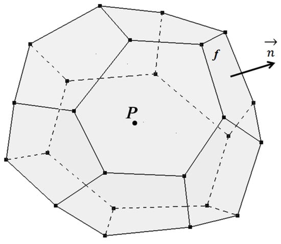
Figure 1.
Cell in the form of a polyhedron.
Navier–Stokes equations in vector form are shown as follows:
where W vector—conservative variables vector, F and G—vectors of convective and diffusive flows, respectively, and H—source term, as follows:
Here, un—normal velocity component, q—heat flow and τij—viscous stress tensor components.
The full description of the set of the Equation (21) approximation method can be found in the work of [29].
Convective flow calculation accuracy is important when solving such problems. As for aerodynamic problems, schemes of the AUSM (advection upstream splitting method) family [30,31] are often used, as is the AUSM + scheme in special cases.
According to [32], in the AUSM + scheme, convective flow over the cell face is determined by the expression:
where cf—sound speed on the face; UL and UR—primitive variables’ vectors on the left and on the right of face f; PL and PR—pressure vector (P = {0, p, 0}T) on the left (L) and on the right (R) of face f; and , , and —scheme parameters.
For the convective flows’ calculation, it is necessary to reconstruct the solution; that is, to determine parameters on the left and on the right of face f. For first-order approximation, values from the cell center (Figure 2) are taken as parameters on the left and on the right of the face:
where and —parameter values on the left and on the right of the face, respectively; and —parameter values in E and P cells’ centers (Figure 2); and —distances from E and P cells’ centers to f face center; and — gradient values in E and P cells; and and —functions-limiters, applied in order to lower oscillation values on discontinuous solutions. The function is used to limit gradient value (to lower gradient value, multiplying it by value αf ≤ 1) and applied to reconstruct parameters on the left and on the right of the cell face [33].
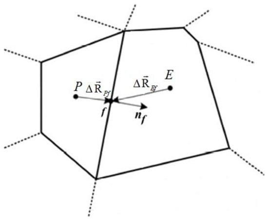
Figure 2.
Value reconstruction scheme.
As mentioned earlier in this article, numerical algorithms, which are adapted for unstructured grid calculations, allow an increase in the range of relevant tasks and the use of numerical simulation when solving problems based on the real geometry of the objects in question. In this article, a hybrid scheme to calculate the gradient of gas-dynamic values is applied to enhance the calculation accuracy for an unstructured grid.
According to this approach, the final gradient value in the cell is determined through the vertical sum of gradients obtained using the Green–Gauss method and the least square method (25):
where —gradient value in cell P, calculated by the least square method, —gradient value in cell P, calculated by the Green–Gauss method, and β—weight function, determining the contribution of each gradient value.
The main difficulty when using the hybrid calculation method is correctly selecting value β. In order to obtain a qualitative gradient value on an unstructured grid, weight function β should have a monotonous dependence character on the cell’s geometrics.
Values of the cell aspect and curvature are factors that affect gradient calculation accuracy. The cell aspect is its maximum and minimum mesh aspect ratio. Value β should depend on both of these cell parameters and provide a smooth transition between two different methods of gradient calculation. Value β is determined as the product of weight values of the cell aspect by cell curvature:
where βAspectCell—weight, determined by the cell aspect; and βcurv—weight, determined by the cell curvature.
where —vector from the center of the cell P to the center of the face f, —normal vector of face f, and min/max—the operation on all faces of the cell.
where α—maximum angle between the face normal and the vector connecting the centers of neighboring cells, and π—number π.
β = βAspectCell × βcurv,
The significance of finding the mesh aspect ratio (i.e., the aspect) is that for degenerated cells (characterized by a greater aspect value) it is preferable to find the gradient by the Green–Gauss method. The greater the weight value of the cell aspect, the greater the contribution of the gradient obtained by the Green–Gauss method. In case of the cell angle of a curvature increase, a greater contribution to the gradient value is made by the gradient obtained by the least square method.
Thus, weight function β’s final value to determine the contribution of each of gradient calculation method takes on values 0 ≤ β ≤ 1. If β = 1, the gradient is calculated by the least square method, if β = 0, it is calculated by the Green–Gauss method.
This approach combines strengths of each gradient calculation method, and takes into account computation cells’ individual characteristics. Thereby, on degenerated and hard-bent cells a more accurate value for the hydrodynamic variable is obtained when interpolating from the cell center onto the face to enhance the order of accuracy (24).
It is also worth mentioning that accuracy of solution deterioration is possible due to insufficient grid resolution, especially in shock waves and the contact discontinuity region. Local grid model refinement realized by a numerical grid adaptation algorithm is one effective way to increase grid resolution. The cell division algorithm underlies the numerical grid adaptation method. It is based on fragmenting the faces that constitute the cell [28] (Figure 3).
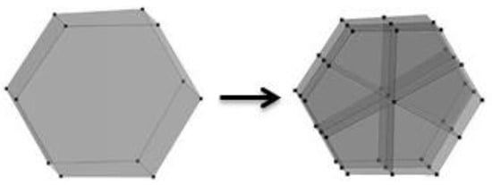
Figure 3.
Cell division in the polyhedral form.
In order to apply an adaptation algorithm, it is necessary to determine refinement regions using adaptation criteria [22].
In order to automatically determine the shock-wave region, originating, for example, from supersonic flow-around, a simple exponential is selected as a relevant criterion (30), with the gas-dynamic gradient value (density, pressure and speed) underlying it.
where Vcell—cell volume, and ∇F—gas-dynamic value gradient.
Value (Vcell)2/3 in expression (30) is used to assess the cell’s geometrics, and takes into consideration criterion f value’s dependence on its volume. Combined with the gas-dynamic value gradient, the maximum criterion value is reached in cells with maximum volume and high gradient value, allowing the inclusion of large cells, lying in the region of the gas-dynamic value’s considerable change (for example, a shock wave), into the local refinement domain. The minimum criterion f value is characteristic of the region, with smooth gas-dynamic values’ changes, and is reached in cells with minimum volume and low gradient value, thus excluding them from the local refinement domain.
The mathematical model based on schemes and algorithms to increase solution accuracy provides qualitative flow structure reproduction when solving problems, including problems on unstructured grids.
3. Research into Shock-Wave Structure of Nozzle Supersonic Flow
Supersonic jet flow from a dissipative nozzle with a narrow throat and cone-expanding section was researched; its geometry is shown in Figure 4 [34].
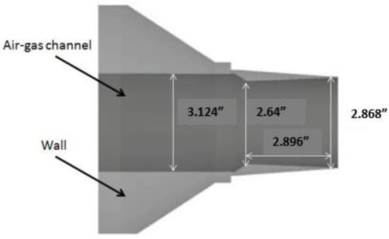
Figure 4.
The nozzle’s general outline and geometry.
The dark field in Figure 4 is the nozzle flow range and the pale (grey) field is the nozzle wall. Diameters at the nozzle inlet, nozzle throat and nozzle outlet are 3.124, 2.64 and 2.868 inches, respectively. The nozzle lip is 0.02 inches thick. The computational region and boundary conditions’ layout are shown in Figure 5.
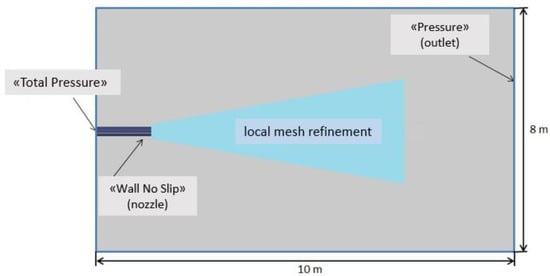
Figure 5.
Computational region’s general outline and boundary conditions’ layout.
Unstructured numerical grids based on truncated hexahedrons (grid A, Figure 6) and polyhedrons (grid B, Figure 7) were constructed for this problem. The total number of cells in grid A is 2.737 mln., while in grid B it is 2.959 mln. Local refinement regions in both numerical grids are located around the nozzle section and continue along the jet flare axis downstream. A cone with 0.07 m and 0.5 m radii, 2.4 m length and 0.0025 m local cell size was set as a local refinement block. During the calculation process, in the local refinement region two levels of grid adaptation to flow features were used to assess the jet’s basic characteristics’ dependence on the grid computation cell’s size.
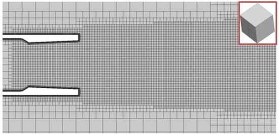
Figure 6.
Base mesh A.
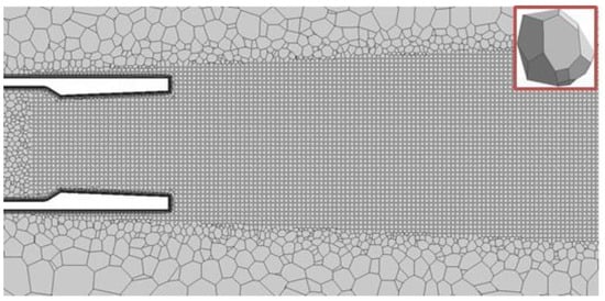
Figure 7.
Base mesh B.
Total pressure and total temperature were set as boundary conditions at the nozzle inlet, according to experimental conditions [34]. In order to carry out this research, the mode with cold jet discharge (300 K) and parameters shown in Table 1 were selected.

Table 1.
Gas parameters.
Figure 8, Figure 9, Figure 10, Figure 11, Figure 12 and Figure 13 show velocity and density for flow parameters from Table 1 for grids A and B. Downstream in the nozzle section there is a train of barrels (a sequence of shock waves), and the potential jet core ends at 12 D distance (D—nozzle exit diameter). In addition, one can see that compression and expansion waves start inside the nozzle, a short distance downstream of the nozzle’s throat.
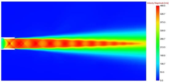
Figure 8.
Velocity field (grid A).
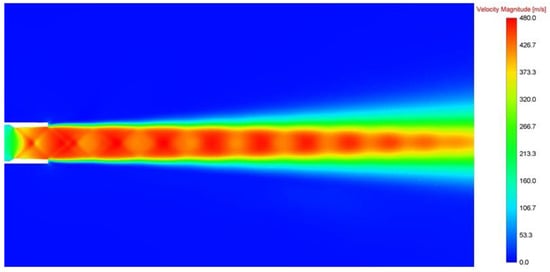
Figure 9.
Velocity field (grid B).
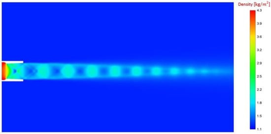
Figure 10.
Density field (grid A).
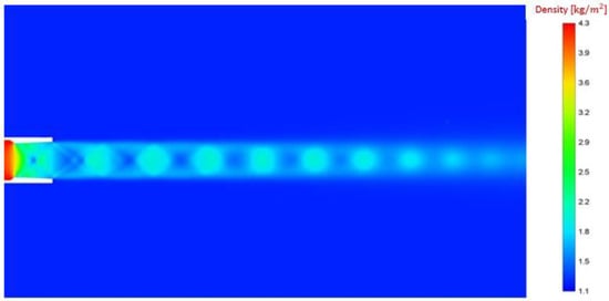
Figure 11.
Density field (grid B).
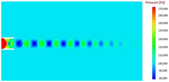
Figure 12.
Static pressure (grid A).
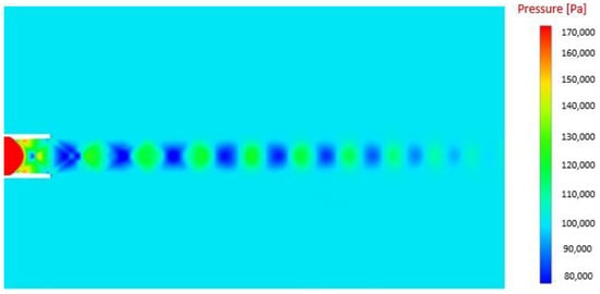
Figure 13.
Static pressure (grid B).
There was a difference in results from different grids in the tail area of the jet. On a grid of polyhedrons, the jet diffused more.
According to [35], the supersonic jet shock-wave structure is outlined in Figure 14.
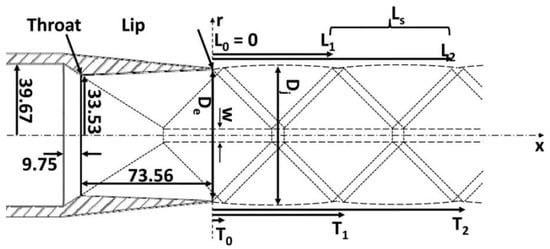
Figure 14.
Supersonic jet structure.
The connection between the second barrel length (Ls) and the fully expanded jet diameter (Dj) is expressed by the following formulas:
where (31) is the Prandtl–Pack model [36] and (32) is a Norum and Seiner elaboration [5] for the C-D nozzle.
However, a basic grid does not have sufficient grid resolution to precisely measure the jet’s geometrical characteristics and find the connection between the second barrel length and the jet’s diameter (Figure 15 and Figure 16).
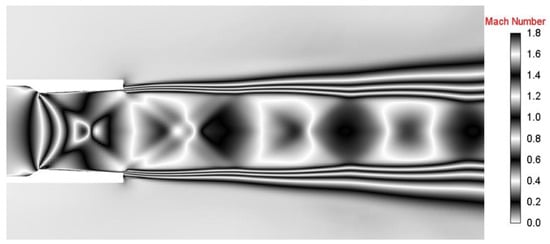
Figure 15.
Mach number distribution, black and white pallet (grid A).
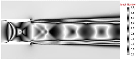
Figure 16.
Mach number distribution, black and white pallet (grid B).
In order to obtain a more precise and coherent flow picture, let us apply the numerical grid static adaptation method (by software LOGOS [https://logos-support.ru/logos/aero-hydro/] to the flow features. Second-level adaptive grids and Mach number distribution fields are shown in Figure 17, Figure 18, Figure 19, Figure 20, Figure 21 and Figure 22.
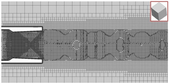
Figure 17.
Second-level adaptive grid (grid A).
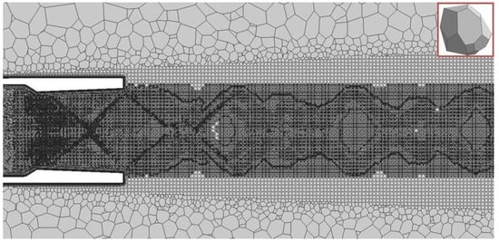
Figure 18.
Second-level adaptive grid (grid B).
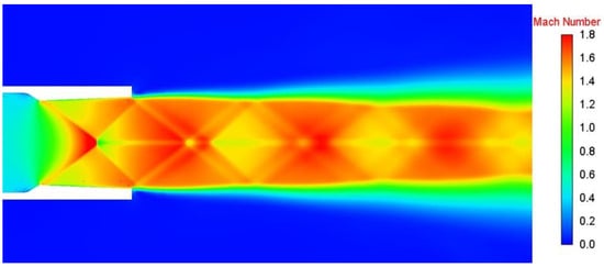
Figure 19.
Mach number distribution (grid A).
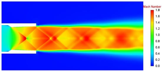
Figure 20.
Mach number distribution (grid B).
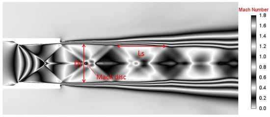
Figure 21.
Mach number distribution, black and white pallet (second-level adaptive grid A).
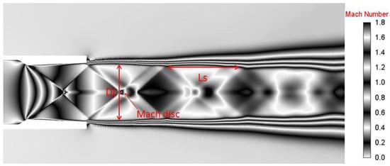
Figure 22.
Mach number distribution, black and white pallet (second-level adaptive grid B).
Building local refinement improved solution accuracy and allowed the use of expression (32) to find the connection between the second barrel length and the fully expanded jet diameter (Figure 21 and Figure 22). Calculation on a more detailed grid revealed the element in the flow as a Mach disk. Figure 23 shows a longitudinal velocity radial profile, in which one can see the central region of the increased velocity modulus.
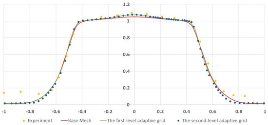
Figure 23.
Longitudinal velocity radial distribution.
It is noteworthy that this result became apparent after the adaptation algorithm was used. In figure results for A and B grids, these results repeated, and so are represented by one caption.
A comparable accuracy result can be obtained on a grid built in a grid generator by setting a smaller cell size in the local refinement region. However, in doing so, a too detailed model is built, which lowers the calculation’s efficiency. In order to research the value of efficiency when using numerical grid A’s adaptation algorithm, let us assess the region meeting adaptation criteria and reproduce it in the grid generator in the form of a geometrical figure.
As a result of applying adaptation criteria according to the gradient of pressure with a maximum 5 × 10⁻⁵ value, the region shown in Figure 24 was selected for numerical grid refinement.
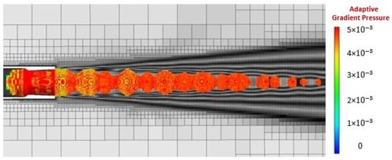
Figure 24.
The region selected by adaptation criteria.
As soon as the barrel sequence in the jet flare has an axisymmetric form, this region can more accurately be described as a truncated cone, which is used to build local refinement in the grid generator. Using the adaptation algorithm and building the grid considering the refinement region as the form of a cone resulted in the following numerical grids (Figure 25).
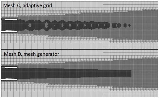
Figure 25.
Grids with local refinement regions.
Grid C’s dimension comprises 3,626,762 cells, and grid D’s comprises 4,333,243 cells. According to calculation results, the following velocity modulus fields were obtained from these grids (Figure 26).
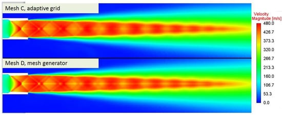
Figure 26.
Velocity modulus distribution (grids C and D).
Figure 27 shows the longitudinal velocity radial profile in Section 2, 15 D for calculations on grid C and grid D.
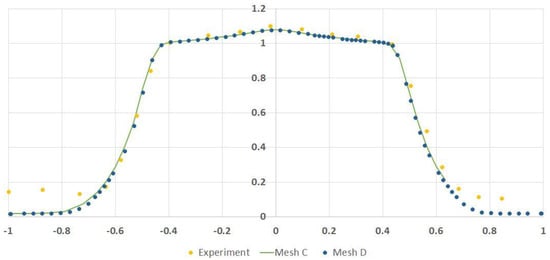
Figure 27.
Longitudinal velocity radial distribution in Section 2, 15 D.
According to these figures, results obtained using grids C and D coincide. In both calculations, solutions were obtained through 400 iterations. However, on grid C the single iteration time was 0.59 s, while on grid D it was 0.71 s. Thus, with the same solver parameters and the same number of iterations, applying grid C improved calculation efficiency by 16.9% due to the numerical solution’s increased speed. General characteristics of calculations on grids C and D are shown in Table 2.
Table 2.
Characteristics of calculations on grids C and D.
This class of problems is highly acute and relevant, as it allows the demonstration of jet flows’ features (for example, the connection between the nozzle geometry and intensity of shock waves in a jet) while jet engines are in operation in real conditions without conducting experiments. The static adaptation algorithm described herein might appear useful to boost the efficiency of such studies.
4. Conclusions
This article presents a physico-mathematical model of supersonic jet flow numerical simulation in order to research the flow structure’s formation. The mathematical model applied was based on the Navier–Stokes set of equations. The hybrid scheme of calculating gas-dynamic values’ gradient was applied to enhance calculation accuracy for an unstructured grid. The numerical grid static adaptation algorithm in the high gradient region of gas-dynamic values was applied to increase grid resolution and build a calculation model with an optimum number of cells.
Jet flow simulation with a 1.56 design Mach number was researched. Calculation results found shock waves in the flow that facilitated obtaining a qualitative description of the flow structure. In addition, calculations on an unstructured grid identified the Mach disc’s position in the flow. A longitudinal velocity profile was presented to assess the solution accuracy. The results obtained agree with experimental data.
The results and approaches presented herein can be used at the air vehicle design stage to determine which nozzle configuration and operation modes provide shock-free flow formation to meet safety standards.
Author Contributions
Conceptualization, A.K. (Andrey Kozelkov) and A.K. (Andrey Kurkin); data curation, A.S. and A.K. (Aleksandr Kornev); formal analysis, A.K. (Andrey Kozelkov) and A.S.; investigation, A.K. (Andrey Kozelkov), A.K. (Andrey Kurkin), A.S. and A.K. (Aleksandr Kornev); methodology, A.K. (Andrey Kozelkov) and A.K. (Andrey Kurkin); software, A.S. and A.K. (Aleksandr Kornev); supervision, A.K. (Andrey Kurkin); validation, A.S. and A.K. (Aleksandr Kornev); visualization, A.S. and A.K. (Aleksandr Kornev); writing–original draft, A.K. (Andrey Kozelkov) and A.K. (Andrey Kurkin); writing—review and editing, A.K. (Andrey Kozelkov) and A.K. (Andrey Kurkin). All authors have read and agreed to the published version of the manuscript.
Funding
This research was funded by the Ministry of Science and Higher Education of the Russian Federation (project No. FSWE-2024-0001 (research topic: «Developing numerical methods, models and algorithms to describe liquid and gas flows in natural environment, and in the context of industrial objects’ operation in standard and emergency conditions on mainframes with exa- and zeta capacity»)) and the scientific program of the National Center of Physics and Mathematics, line No. 2 «Mathematical modelling on mainframes with exa- and zeta capacity. Stage 2023–2025».
Data Availability Statement
The original contributions presented in the study are included in the article, further inquiries can be directed to the corresponding author.
Conflicts of Interest
The authors declare no conflicts of interest.
References
- Kozelkov, A.S.; Strelets, D.Y.; Sokuler, M.S.; Arifullin, R.H. Application of Mathematical Modeling to Study Near-Field Pressure Pulsations of a Near-Future Prototype Supersonic Business Aircraft. J. Aerosp. Eng. 2022, 35, 04021120. [Google Scholar] [CrossRef]
- Tam, C.K.W.; Tanna, H.K. Shock associated noise of supersonic jets from convergent-divergent nozzles. J. Sound Vib. 1982, 81, 337–358. [Google Scholar] [CrossRef]
- Tam, C.K.W. Jet Noise Generated by large Scale Coherent Motion. In NASA. Langley Research Center, Aeroacoustics of Flight Vehicles: Theory and Practice; Hubbard, H.H., Ed.; National Aeronautics and Space Administration: Washington, DC, USA, 1991; Volume 1: Noise Sources, pp. 311–390. [Google Scholar]
- Tam, C.K.W. Supersonic Jet Noise. Annu. Rev. Fluid Mech. 1995, 27, 17–43. [Google Scholar] [CrossRef]
- Norum, T.D.; Seiner, J.M. Broadband Shock Noise from Supersonic Jets. AIAA J. 1982, 20, 68–73. [Google Scholar] [CrossRef]
- Raman, G. Advances in Understanding Supersonic Jet Screech: Review and Perspective. Prog. Aerosp. Sci. 1998, 34, 45–106. [Google Scholar] [CrossRef]
- Umeda, Y.; Ishii, R. On the Sound Sources of Screech Tones Radiated from Choked Circular Jets. J. Acoust. Soc. Am. 2001, 110, 1845–1858. [Google Scholar] [CrossRef] [PubMed]
- Bodony, D.J.; Lele, S.K. On Using Large-Eddy Simulation for the Prediction of Noise from Cold and Heated Turbulent Jets. Phys. Fluids 2005, 17, 085103. [Google Scholar] [CrossRef]
- Bogey, C.; Bailly, C. Effects of Inflow Conditions and Forcing on Subsonic Jet Flows and Noise. AIAA J. 2005, 43, 1000–1007. [Google Scholar] [CrossRef][Green Version]
- Freund, J.B. Noise Sources in a Low-Reynolds-Number Turbulent Jet at Mach 0.9. J. Fluid Mech. 2001, 438, 277–305. [Google Scholar] [CrossRef]
- Uzun, A.; Blaisdell, G.A.; Lyrintzis, A.S. Coupling of Integral Acoustics Methods with LES for Jet Noise Prediction. Int. J. Aeroacoustics 2004, 3, 297–346. [Google Scholar] [CrossRef]
- Bodony, D.J.; Lele, S.K. Current Status of Jet Noise Predictions Using Large-Eddy Simulation. AIAA J. 2004, 46, 364–380. [Google Scholar] [CrossRef]
- DeBonis, J.R.; Scott, J.N. A Large-Eddy Simulation of a Turbulent Compressible Round Jet. AIAA J. 2002, 40, 1346–1354. [Google Scholar] [CrossRef]
- Andersson, N.; Eriksson, L.; Davidson, L. Large-Eddy Simulation of Subsonic Turbulent Jets and Their Radiated Sound. AIAA J. 2005, 43, 1899–1912. [Google Scholar] [CrossRef]
- Vuillot, F.; Lupoglazoff, N.; Rahier, G. Double-Stream Nozzles Flow and Noise Computations and Comparisons to Experiments. In Proceedings of the 46th AIAA Aerospace Sciences Meeting and Exhibit, Reno, Nevada, 7–10 January 2008. [Google Scholar]
- Xia, H.; Tucker, P.G.; Eastwood, S. Towards Jet Flow LES of Conceptual Nozzles for Acoustic Predictions. In Proceedings of the 46th AIAA Aerospace Sciences Meeting and Exhibit, Reno, Nevada, 7–10 January 2008. [Google Scholar]
- Shur, M.L.; Spalart, P.R.; Strelets, M.K.; Garbaruk, A.V. Further Steps in LES-Based Noise Prediction for Complex Jets. In Proceedings of the 44th AIAA Aerospace Sciences Meeting and Exhibit, Reno, Nevada, 9–12 January 2006. [Google Scholar]
- Viswanathan, K.; Shur, M.L.; Spalart, P.R.; Strelets, M.K. Computation of the Flow and Noise of Round and Beveled Nozzles. In Proceedings of the 12th AIAA/CEAS Aeroacoustics Conference (27th AIAA Aeroacoustics Conference), Cambridge, MA, USA, 8–10 May 2006. [Google Scholar]
- Bodony, D.J.; Ryu, J.; Lele, S.K. Investigating Broadband Shock-Associated Noise of Axisymmetric Jets Using Large-Eddy Simulation. In Proceedings of the 12th AIAA/CEAS Aeroacoustics Conference (27th AIAA Aeroacoustics Conference), Cambridge, MA, USA, 8–10 May 2006. [Google Scholar]
- Lo, S.C.; Blaisdell, G.A.; Lyrintzis, A.S. Numerical Simulation of Supersonic Jet Flows and their Noise. In Proceedings of the 14th AIAA/CEAS Aeroacoustics Conference (27th AIAA Aeroacoustics Conference), Vancouver, BC, Canada, 5–7 May 2008. [Google Scholar]
- Imamoglu, B.; Balakumar, P. Computation of Shock Induced Noise in Imperfectly Expanded Supersonic Jets. Int. J. Aeroacoustics 2007, 6, 127–146. [Google Scholar] [CrossRef]
- Struchkov, A.V.; Kozelkov, A.S.; Volkov, K.N.; Kurkin, A.A.; Zhuchkov, R.N.; Sarazov, A.V. Numerical simulation of aerodynamic problems based on adaptive mesh refinement method. Acta Astronaut. 2020, 172, 7–15. [Google Scholar] [CrossRef]
- Struchkov, A.V.; Kozelkov, A.S.; Zhuchkov, R.N.; Volkov, K.N.; Strelets, D.Y. Implementation of Flux Limiters in Simulation of External Aerodynamic Problems on Unstructured Meshes. Fluids 2023, 8, 31. [Google Scholar] [CrossRef]
- Dmitriev, S.M.; Kozelkov, A.S.; Kurkin, A.A.; Legchanov, M.A.; Tarasova, N.V.; Kurulin, V.V.; Efremov, V.R.; Shamin, R.V. Simulation of turbulent convection at high Rayleigh numbers. Model. Simul. Eng. 2018, 2018, 5781602. [Google Scholar] [CrossRef]
- Deryugin, Y.N.; Zhuchkov, R.N.; Zelenskiy, D.K.; Kozelkov, A.S.; Sarazov, A.V.; Kudimov, N.F.; Lipnickiy, Y.M.; Panasenko, A.V.; Safronov, A.V. Validation Results for the LOGOS Multifunction Software Package in Solving Problems of Aerodynamics and Gas Dynamics for the Lift-Off and Injection of Launch Vehicles. Math. Models Comput. Simul. 2015, 7, 144–153. [Google Scholar] [CrossRef]
- Loitsyanskii, L.G. Mechanics of Liquids and Gases. In International Series of Monographs in Aeronautics and Astronautics, Division II, Aerodynamics, 2nd ed.; Pergamon Press: New York, NY, USA, 1966; Volume 6. [Google Scholar]
- Jasak, H. Error Analysis and Estimation for the Finite Volume Method with Applications to Fluid Flow; Department of Mechanical Engineering, Imperial College of Science: London, UK, 1996. [Google Scholar]
- Spalart, P.R.; Allmaras, S.R. A one-equation turbulence model for aerodynamic flows. In Proceedings of the 30th AIAA Aerospace Sciences Meeting and Exhibit, Reno, Nevada, 6–9 January 1992. [Google Scholar]
- Ferziger, J.H.; Peric, M. Computational Method for Fluid Dynamics; Springer: New York, NY, USA, 2002. [Google Scholar]
- Liou, M.-S. A Sequel to AUSM: AUSM+. J. Comput. Phys. 1996, 129, 364–382. [Google Scholar] [CrossRef]
- Vierendeels, J.; Merci, B.; Dick, E. Blended AUSM+ Method for All Speeds and All Grid Aspect Ratios. AIAA J. 2001, 39, 2278–2282. [Google Scholar] [CrossRef]
- Kim, K.H.; Kim, C.; Rho, O.-H. Methods for the accurate computations of hypersonic flows. I AUSMPW+ scheme Methods. J. Comput. Phys. 2001, 174, 38–80. [Google Scholar] [CrossRef]
- Sweby, P.K. High resolution using flux limiters for hyperbolic conservation laws. SIAM J. Numer. Anal. 1984, 21, 995–1011. [Google Scholar] [CrossRef]
- Liu, J.; Kailasanath, K.; Ramamurti, R.; Munday, D.; Gutmark, E.; Lohner, R. Large-Eddy Simulations of a Supersonic Jet and Its Near-Field Acoustic Properties. AIAA J. 2009, 47, 1849–1864. [Google Scholar] [CrossRef]
- Munday, D.; Gutmark, E.; Liu, J.; Kailasanath, K. Flow structure and acoustics of supersonic jets from conical convergent-divergent nozzles. Phys. Fluids 2011, 23, 116102. [Google Scholar] [CrossRef]
- Pack, D.C. A note on Prandtl’s formula for the wavelength of a supersonic gas jet. Q. J. Mech. Appl. Math. 1950, 3, 173–181. [Google Scholar] [CrossRef]


Disclaimer/Publisher’s Note: The statements, opinions and data contained in all publications are solely those of the individual author(s) and contributor(s) and not of MDPI and/or the editor(s). MDPI and/or the editor(s) disclaim responsibility for any injury to people or property resulting from any ideas, methods, instructions or products referred to in the content. |
© 2024 by the authors. Licensee MDPI, Basel, Switzerland. This article is an open access article distributed under the terms and conditions of the Creative Commons Attribution (CC BY) license (https://creativecommons.org/licenses/by/4.0/).