Pressure and Velocity Profiles over a Weir Using Potential Flow Model

Abstract

A potential flow model of the semi-inverse type is proposed to simulate flow over round crested weirs. This technique involves the construction of only streamlines over the weir instead of constructing the entire flow net. A Serre–Green–Naghdi (SGN) equation is employed to determine the initial free-surface profile, which is solved using a combined finite volume-finite difference scheme. The potential flow equations were numerically solved using a five-point central finite difference scheme. The model was applied to define the pressure and velocity fields in channel controls involving transcritical flow, such as the Gaussian weir, parabolic weir, and semicircular weir. The impact of streamline curvature on pressure and velocity distributions was investigated in the study. The curvature of the streamline strongly influenced the rise and drop of the bed pressures along the test section. A semicircular weir experiment was also conducted to validate the pressure and velocity profiles obtained using the proposed 2-D fluid flow model. The computed pressure and flow profiles from the solution of the potential flow equation agree perfectly with the present experiment and similar experiments available in the literature. In conclusion, the SGN equation provides an excellent initial profile to solve a 2-D ideal fluid flow numerically.

1. Introduction

Weirs are the best hydraulic structures widely used for water discharge measurements due to their ability to measure a wide range of flow. The shape of the crest in the flow direction classifies weirs, which are then further subdivided based on the cross-sections of the crest. Among these, short-crested weirs differ significantly from the broad-crested weirs and the sharp-crested weirs characterized by sharply bent streamlines and non-hydrostatic pressure conditions across stream nappe over the crest surface [1]. The centrifugal force induced by the stream curvature in transcritical flow over the weir forms a non-hydrostatic pressure and non-uniform velocity [2,3]. Transcritical flow is an undular flow motion observed when the flow depth is close to the critical depth in an open channel; a small change in specific energy can induce a large change in flow depth. Incompressible, non-viscous, and irrotational flow equations are used to describe the transition of flow from subcritical to supercritical throughout a critical point [4]. The potential flow theory, a simple mathematical model to obtain the detailed flow features, assumes the flow is inviscid and irrotational, as compared with the advanced turbulence model [5]. The potential flow model involves determining the potential and stream functions at every location in the flow domain, thereby generating pressure and velocity fields [2,6,7]. Furthermore, Rouse [6] and, more recently, Pu et al. [8], Pu [9], and Zheng et al. [10] used various incompressible, non-viscous, irrotational flow and turbulence equations to describe the 2D flow behaviour of open channel flow.

The availability of experimental data in transcritical flow to describe the flow profile, velocity, and pressure distributions is limited. Messe [11] demonstrated that transition from subcritical to supercritical regimes is possible with a continuous surface profile and finite surface slope while maintaining the hydrostatic-pressure distribution. Andersen [12] investigated the flow curvature’s influence on the non-hydrostatic pressure profile at the location where a change in slope occurs. The relaxation approach was utilized by Southwell and Vaisey [13] to solve the partial differential equation for the stream function $\psi$ on the physical plane ($x,y$). But solving the Laplace equation on physical plane $(x,y)$ is very difficult. Markland [14] solved the Laplace equation for dependent variables $x$ and $y$ in this complex potential plane $\left(\varphi ,\psi \right)$ using a finite difference technique and a relaxation procedure for spillways and free overfall problems. However, discretizing the equation over curved beds and selecting an effective relaxation pattern are time-consuming processes [15]. Chan et al. [16] utilized the finite element approach to model flow under gates. Cheng et al. [17] used the boundary integral approach to model flow across spillways. A different approach was suggested by Thom and Apelt [15], transforming the relationship between dependent and independent variables where a rectangular strip on the complex potential plane was used to map the real plane. Chow and Han [18] used an approach where the hodograph of free overfall was plotted on a rectangular strip, solving the Laplace equation for stream function with hodograph variables as an independent variables using relaxation techniques.

The Laplace equation for $\psi$ on the physical plane ($x,y$) was modified by Boadway [19] into a relation that expresses $y$ as a function of $\psi$ and $x$. Montes [20] used this semi-inverse transformation of the Laplace equation derived by Boadway to simulate flow over curved beds. A review of existing potential flow solutions focused on flow profile and bottom-pressure simulations, and they were not employed to examine other internal flow properties [21,22]. Castro-Orgaz [22] used the Boadway model for analyzing transcritical flow over a weir where specific energy is the minimum at the crest. Due to the existence of an uneven free surface, the potential flow solution for open-channel flow is complicated [22,23]. Castro-Orgaz [22] also considered the Boussinesq-type energy equation to estimate the initial flow profile.

The flow curvature formed over a round-crested control structure results in non-uniform velocity and non-hydrostatic pressure [2]. The divergence of pressure from hydrostatic conditions is not applicable to the Saint-Venant equation in these structures [24]. For shallow flows with a horizontal channel bottom or with minimum inclination $\theta$, Saint-Venant equations provide reasonable approximations of solutions [25]. The Saint-Venant equations, as modified by Boussinesq [26], included the curvature effect on particle velocities. Dressler [25] derived the generalized nonlinear shallow-flow equations in a bottom-fitted curvilinear coordinate system. Dressler-derived equations simplified the Saint-Venant approach for channel reaches by having a constant bottom slope [27]. On the other hand, Naghdi and Vongsarnpigoon [28] numerically solved the Boussinesq-type energy equation, where the model was applied to a rigid hump case. Matthew [29] derived a higher-order equation for potential flow in open channels in Cartesian coordinates using Picard’s iterative procedure. It was found that in the Bernoulli solver, the presumed upstream flow depth of the hydrostatic condition is insensible, causing the downstream flow depth and total head calculations to be error-prone [30]. The advantage of the Serre–Green–Naghdi solver over the Bernoulli solver is that the computed flow profile has less impact through incorrect estimation of upstream flow depth [24]. The Serre–Green–Naghdi (SGN) equations are a set of nonlinear partial differential equations used to model shallow water flow, mostly used in marine hydraulics. There were very few previous applications of a steady or unsteady version of the SGN equation found for modelling flow over round-crested weirs. The SGN equation was first solved for flow over curved beds using a finite volume-finite difference scheme using the MUSCL-Hancock scheme by Castro-Orgaz and Cantero-Chinchilla [31]. The objective of the present study is to utilize the initial profile solved using a similar approach to complete Boadway’s potential flow model. The present study differs from the previous potential flow model by Montes [20,32] and Castro-Orgaz [22] by preferring the Serre–Green–Naghdi equation over the Bernoulli-type Boussinesq equation to determine the initial free surface profile. An experiment is conducted to determine velocity and pressure profiles at selected sections of the semicircular weir in detail. Also, a 2-D ideal fluid flow solution is used to validate velocity and pressure profiles by the present experimental work to show the curvature of the streamline effect on pressure profiles at selected sections of the semicircular weir in detail.

2. Governing Equation

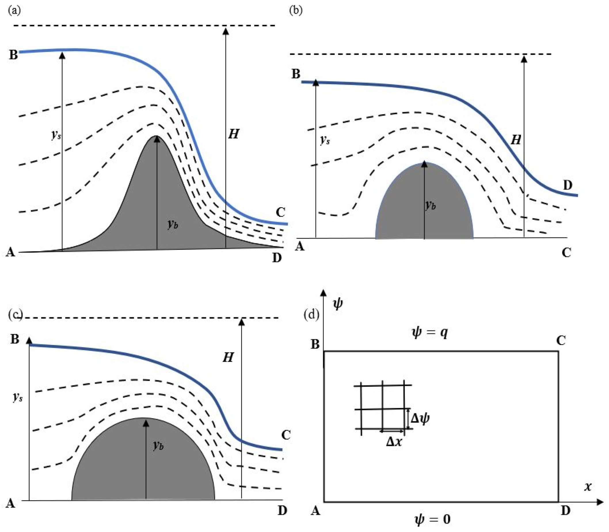
2.1. The $x$-$\psi$ Transformation

Southwell and Vaisey [13] considered the Laplace equation for $\psi$ on the $x$-$y$ plane:

$${\nabla }^2\psi ={\displaystyle \frac{{\partial }^2\psi }{\partial x^2}}+{\displaystyle \frac{{\partial }^2\psi }{\partial y^2}}=0$$

(1)

where ${\nabla }^2$ is a second-order differential operator commonly known as the Laplacian operator. As mentioned earlier, an irregular computational mesh was required to solve the equation; therefore, the process of solution in the physical plane near curved boundary streamlines was laborious [15,22]. Boadway [19] transformed Equation (1) into a relationship expressing $y$ as a function of $\psi$ and $x$. The advantage of this kind of transformation is that the initial free surface profile may be specified considerably more easily as a function of $x$ than that of $\varphi$. BC in Figure 1 represents the free surface, and AB and CD are two vertical sections where the potential flow is assumed to be parallel to the boundary with uniform velocity and hydrostatic-pressure distributions. This geometry is represented by the $x$-$\psi$ plane rectangular strip ABCD. The semi-inverse transformation of the Laplace equation $y=y(x,\psi )$ is expressed as [19]:

$${\nabla }^{2}y={\displaystyle \frac{{\partial }^{2}y}{\partial x^2}}{\left({\displaystyle \frac{\partial y}{\partial \psi }}\right)}^2+{\displaystyle \frac{{\partial }^{2}y}{\partial {\psi }^2}}\left[1+{\left({\displaystyle \frac{\partial y}{\partial x}}\right)}^2\right]-2{\displaystyle \frac{{\partial }^{2}y}{\partial x\partial \psi }}{\displaystyle \frac{\partial y}{\partial x}}{\displaystyle \frac{\partial y}{\partial \psi }}=0$$

(2)

Boadway’s mapping allows modellers to simplify the complete flow net to only determine the streamline pattern; as a result, the potential function can be ignored [22]. The potential flow’s velocity and pressure distributions are generated once the equation for each streamline has been solved. The vertical and horizontal velocity components in terms of $x$, $y$ and $\psi$ are

$$v=u{\displaystyle \frac{\partial y}{\partial x}}$$

(3)

$$u={\displaystyle \frac{\partial \psi }{\partial y}}$$

(4)

2.2. Boundary Conditions

2.2.1. Upstream and Downstream Boundaries

The boundary conditions are taken at where streamlines are aligned with the channel bottom. They are given as follows: (1) The vertical ordinate $y(x,0)$ at all points in the lower boundary, where $\psi =$0 is prescribed by $y_b$; (2) the vertical ordinates $y(x_0,q)$ and $y(x_n,q)$ at upstream and downstream sections of the free surface, respectively. Let $j$ represent the mesh’s node index in the $\psi$-direction, as shown in Figure 2. The variation of $y$ at point $j$ in the upstream and downstream sections is given by Equation (5)

$$y_j=y_b+∆y\left({\displaystyle \frac{{\psi }_j}{{\psi }_n}}\right)$$

(5)

2.2.2. Free Surface Boundary

The first step in a potential flow model is determining the initial flow profile which is a crucial part of the model. Previous potential flow solvers utilized experimental data or initial profiles obtained from other models to estimate the initial flow profile [22]. It is an essential step because it determines the solution’s accuracy. The selection of a poor initial flow profile could lead to the failure of the solution. Montes [32] used the energy equation to find the vertical ordinate $y$ of the free surface.

$$y=H-y_b-{\displaystyle \frac{u_s^2}{2g}}\left(1+{\left({\displaystyle \frac{d{y}_b}{dx}}\right)}^2\right)$$

(6)

where $y_b=$ bed elevation; ${\psi }_n=q$; $H$ = total head; $y$ = water depth; $g$ = acceleration due to gravity; and $u_s$ = horizontal surface velocity. Castro-Orgaz [22] recommended an initial free-surface $y_s$ and energy head $H$ for the selected discharge per unit width $q$ to start the potential flow solution. He used a second-order equation for potential flow developed by Matthew [29], similar to that of the Boussinesq-type Bernoulli equation, to obtain the initial free-surface profile.

$$H=y_b+y+{\displaystyle \frac{q^2}{2g{y}^2}}\left(1+{\displaystyle \frac{2y\left(d^{2}y/d{x}^2\right)-{\left(dy/dx\right)}^2}{3}}+y\left(d^2{y}_b/d{x}^2\right)+{\left(d{y}_b/dx\right)}^2\right)$$

(7)

where $x$ is the longitudinal space coordinate; $d/dx$ indicates ordinary differentiation with respect to $x$. The above equation considers the hydrostatic condition $H=y_1+{\displaystyle \frac{q^2}{2g{y}_1^2}}$ as one of the boundary conditions, which assumes ${\displaystyle \frac{dy}{dx}}={\displaystyle \frac{d^{2}y}{d{x}^2}}=0$ at $x=x_1.$ However, if the upstream water depth $y_1$ is inaccurate, then $d^{2}y/d{x}^2\ne 0$, and nonlinear and periodic waves will occur upstream, causing the calculation of $H$ to be incorrect, too [24]. As proven, the error involved with the incorrect estimation of upstream flow depth is lesser in the SGN solver [24]. This paper adopts a steady SGN solver to estimate the initial flow profile over curved beds to start the solution of Boadway’s semi-inverse transformation of the Laplace equation.

The SGN equations are widely employed to calculate shallow and moderate ocean waves [24,33,34]. The free surface analysis in the undular jumps is one of the applications of the steady SGN equations in open-channel hydraulics by Hosoda and Tada [35] and in depth-averaged flow models to estimate dune form and flow resistance by Onda and Hosoda [36]. Castro-Orgaz and Cantero-Chinchilla [31] were the first to apply the steady and unsteady versions of the SGN equation to compute the flow characteristics over curved beds. The steady SGN for 1D water waves travelling across any topography [31,36]:

$$\begin{gathered} {\displaystyle \frac{d}{dx}}\left[{\displaystyle \frac{y^2}{2}}+{\displaystyle \frac{q^2}{gy}}\left(1+{\displaystyle \frac{y\left(\frac{d^{2}y}{d{x}^2}\right)-{\left(\frac{dy}{dx}\right)}^2}{3}}+{\displaystyle \frac{y\left(\frac{d^2{y}_b}{d{x}^2}\right)}{2}}-{\displaystyle \frac{\left(\frac{dy}{dx}\right)\left(\frac{d{y}_b}{dx}\right)}{2}}\right)\right]=-\left[y+{\displaystyle \frac{q^2}{2g{y}^2}}\left(2y\left(d^2{y}_b/d{x}^2\right)+y\left(d^{2}y/d{x}^2\right)- \\ {\left(dy/dx\right)}^2-2\left(d{y}_b/dx\right)\left(dy/dx\right)\right)\right]{\displaystyle \frac{d{y}_b}{dx}}. \end{gathered}$$

(8)

Equation (7) is the first integral of Equation (8), where total head $H$ is the constant of integration of Equation (8). This relation is verified by differentiating Equation (8) once with respect to $x$(the derivation is given in Appendix A). Both differential equation features are different during numerical simulations; however, they produce the same final converged solutions after the correct estimation of upstream flow depth [24]. Equation (9) is obtained after neglecting the second-order products in derivatives of $y$ and $y_b$, as is shown in Appendix B.

$${\displaystyle \frac{q^2}{g}}\left({\displaystyle \frac{1}{3}}\left(d^{3}y/d{x}^3\right)+{\displaystyle \frac{1}{2}}\left(d^2{y}_b/d{x}^2\right)\right)+\left(y-{\displaystyle \frac{q^2}{g{y}^2}}\right)\left(dy/dx\right)=-y\left(d{y}_b/dx\right).$$

(9)

Equation (9) is a third-order ordinary differential equation which requires three boundary conditions. Komai [37] set the experimental values of flow depth as boundary conditions in upstream and downstream sections and $dy/dx=0$ at the upstream section and solved the system of implicit non-linear equations by the Newton–Raphson iteration technique. A similar procedure is adopted in this work to solve the non-linear implicit equation to obtain an initial flow profile over a curved weir.

3. Solution Techniques

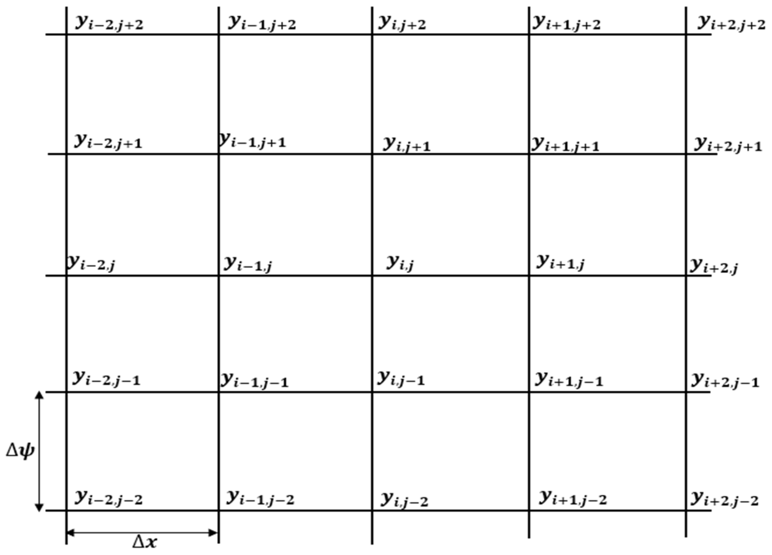
3.1. Solution of $x$-$\psi$ Transformation of Laplace Equation

The solution for the semi-inverse transformation of the Laplace equation for the $y$-coordinate in terms of $\psi$ and $x$ is obtained once all the values of $y$ are prescribed along the contour A-B-C-D-A [Figure 1d] in the computational domain of the $x$-$\psi$ plane. Let $i$ represent the node index of the mesh in the longitudinal direction with grid size $∆x$, and $j$ represent the node index of the mesh in the vertical direction with grid size $∆\psi$ as shown in Figure 2. The five-point finite difference approach [38] was used to estimate the terms for the computational node in the region of the internal boundary section. The partial derivative terms of Equation (2) are replaced with fourth-order accurate central finite difference approximations in order to reduce truncation error (i.e., derivation of Equation (12) is given in Appendix C). They produce higher accuracy by including more considered points when compared to the three-point central finite difference scheme.

$${\displaystyle \frac{\partial y}{\partial x}}={\displaystyle \frac{-y_{i+2,j}+{8y}_{i+1,j}-8y_{i-1,j}+y_{i-2,j}}{12∆x}}$$

(10)

$${\displaystyle \frac{\partial y}{\partial \psi }}={\displaystyle \frac{-y_{i,j+2}+8y_{i,j+1}-8y_{i,j-1}+y_{i,j-2}}{12∆\psi }}$$

(11)

$${\displaystyle \frac{{\partial }^{2}y}{\partial x\partial \psi }}={\displaystyle \frac{1}{144∆x∆\psi }} \left(\begin{array}{c}-y_{i-2,j+2}+8y_{i-2,j+1}-8y_{i-2,j-1}+y_{i-2,j-2}+\\ 8y_{i-1,j+2}-64y_{i-1,j+1}+64y_{i-1,j-1}-8y_{i-1,j-2}\\ {+y}_{i+2,j+2}-8y_{i+2,j+1}+8y_{i+2,j-1}-y_{i+2,j-2}-\\ -8y_{i+1,j+2}+64y_{i+1,j+1}-64y_{i+1,j-1}+8y_{i+1,j-2}\end{array}\right)$$

(12)

$${\displaystyle \frac{{\partial }^{2}y}{\partial x^2}}={\displaystyle \frac{{-y}_{i+2,j}+16y_{i+1,j}-{30y}_{i,j}+16y_{i-1,j}-y_{i-2,j}}{12{(∆x)}^2}}$$

(13)

$${\displaystyle \frac{{\partial }^{2}y}{\partial {\psi }^2}}={\displaystyle \frac{{-y}_{i,j+2}+16y_{i,j+1}-{30y}_{i,j}+{16y}_{i,j-1}-y_{i,j-2}}{12{(∆\psi )}^2}}$$

(14)

$$A_1=-y_{i+2,j}+{8y}_{i+1,j}-8y_{i-1,j}+y_{i-2,j}$$

(15)

$$B_1={-y}_{i+2,j}+16y_{i+1,j}+16y_{i-1,j}-y_{i-2,j}$$

(16)

$$C_1=-y_{i,j+2}+8y_{i,j+1}-8y_{i,j-1}+y_{i,j-2}$$

(17)

$$D_1={-y}_{i,j+2}+16y_{i,j+1}+{16y}_{i,j-1}-y_{i,j-2}$$

(18)

$$E_1={-y}_{i+2,j+2}+8y_{i+2,j+1}-8y_{i+2,j-1}+y_{i+2,j-2}$$

(19)

$$F_1=-8y_{i+1,j+2}+64y_{i+1,j+1}-64y_{i+1,j-1}-8y_{i+1,j-2}$$

(20)

$$G_1=+y_{i-2,j+2}-8y_{i-2,j+1}+8y_{i-2,j-1}-y_{i-2,j-2}$$

(21)

$$H_1=8y_{i-1,j+2}-64y_{i-1,j+1}+64y_{i-1,j-1}-8y_{i-1,j-2}$$

(22)

Substituting Equations (10)–(22) into Equation (2), the system of linear equations results for $y_{i,j}$ at the finite difference mesh’s nodes are written as

$$y_{i,j}={\displaystyle \frac{6B_1\left(C_1^2\right)+6D_1\left(144{\left(∆x\right)}^2+A_1^2\right)-(E_1+F_1+G_1+H_1)\left(A_1\right)\left(C_1\right)}{180\left(C_1^2+A_1^2+144{\left(∆x\right)}^2\right)}}$$

(23)

The convergent solution of Equation (23) is obtained by an iterative method, as the $y_{i,j}$ value is dependent on the four points surrounding the mesh. To avoid fictitious nodes beyond the computational domain, the terms for the computational node in the area of the extreme boundary section were estimated using the three-point finite difference method. Replacing the partial derivatives of Equation (2) by three-point central finite difference approximations such as [20,22,32]:

$${\displaystyle \frac{\partial y}{\partial x}}={\displaystyle \frac{y_{i+1,j}-y_{i-1,j}}{2∆x}}$$

(24)

$${\displaystyle \frac{\partial y}{\partial \psi }}={\displaystyle \frac{y_{i,j+1}-y_{i,j-1}}{2∆\psi }}$$

(25)

$${\displaystyle \frac{{\partial }^{2}y}{\partial x^2}}={\displaystyle \frac{y_{i+1,j}-{2y}_{i,j}+y_{i-1,j}}{{(∆x)}^2}}$$

(26)

$${\displaystyle \frac{{\partial }^{2}y}{\partial {\psi }^2}}={\displaystyle \frac{y_{i,j+1}-{2y}_{i,j}+y_{i,j-1}}{{(∆\psi )}^2}}$$

(27)

$${\displaystyle \frac{{\partial }^{2}y}{\partial x\partial \psi }}={\displaystyle \frac{y_{i+1,j+1}-y_{i-1,j+1}-y_{i+1,j-1}+y_{i-1,j-1}}{4∆x∆\psi }}$$

(28)

$$A^{\prime }=y_{i+1,j}-y_{i-1,j}$$

(29)

$$B^{\prime }=y_{i+1,j}+y_{i-1,j}$$

(30)

$$C^{\prime }=y_{i,j+1}-y_{i,j-1}$$

(31)

$$D^{\prime }=y_{i,j+1}+y_{i,j-1}$$

(32)

$${E^{\prime }=y}_{i+1,j+1}-y_{i-1,j+1}-y_{i+1,j-1}+y_{i-1,j-1}$$

(33)

Substitution of Equations (24)–(33) into Equation (2), the system of linear equations results for $y_{i,j}$ at the nodes of the FD mesh.

$$y_{i,j}={\displaystyle \frac{2B^{\prime }\left({\left(C^{\prime }\right)}^2\right)+2D^{\prime }\left(4{\left(∆x\right)}^2+{\left(A^{\prime }\right)}^2\right)-E^{\prime }\left(A^{\prime }\right)\left(C^{\prime }\right)}{4({\left(C^{\prime }\right)}^2+{\left(A^{\prime }\right)}^2+4{\left(∆x\right)}^2)}}$$

(34)

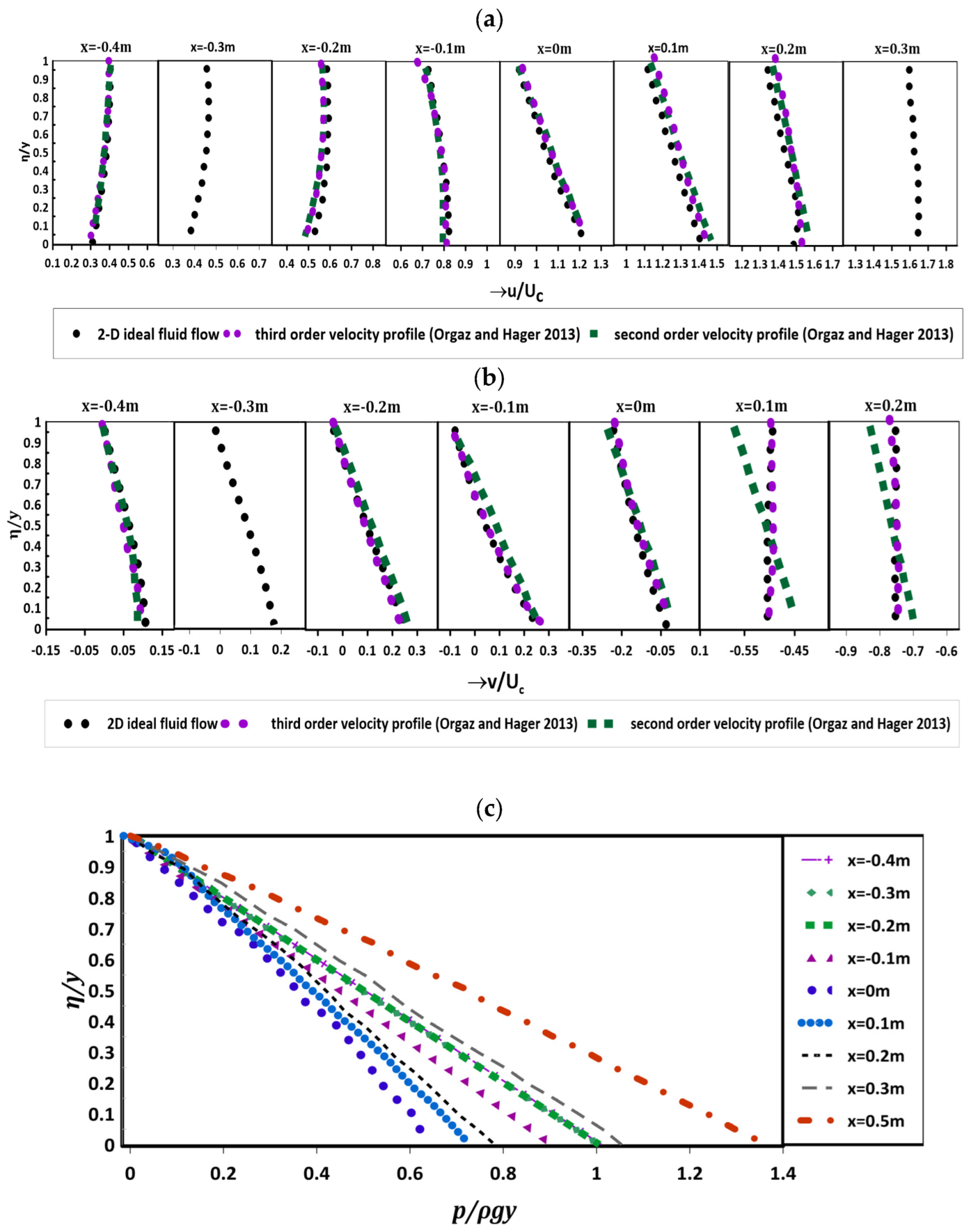
3.2. Velocity and Pressure Distributions

The hydraulic characteristics of flow at transitions with moderate to fast accelerating flow inhibiting the formation of the boundary layer are accurately predicted using potential-flow techniques [32]. After obtaining the values of $y_{i,j}$ at all grid points, the horizontal and vertical velocity fields of the interior nodes are computed from the fourth-order central discretization of Cartesian velocity components:

$$u_{i,j}={\displaystyle \frac{12∆\psi }{-y_{i,j+2}+8y_{i,j+1}-8y_{i,j-1}+y_{i,j-2}}}$$

(35)

$$v_{i,j}=u_{i,j}{\displaystyle \frac{-y_{i+2,j}+8y_{i+1,j}-8y_{i-1,j}+y_{i-2,j}}{12∆x}}$$

(36)

Let $N$ represent the highest value of $j$ at the free surface. The horizontal velocity at the free surface and bottom are computed from the fourth-order discretization with the five-point one-sided stencil scheme:

$$u_s={\displaystyle \frac{12∆\psi }{{25y}_{i,N}-4{8y}_{i,N-1}+36y_{i,N-2}-16y_{i,N-3}+3y_{i,N-4}}}$$

(37)

$$u_b={\displaystyle \frac{12∆\psi }{-25y_{i,0}+4{8y}_{i,1}-{36y}_{i,2}+16y_{i,3}-3y_{i,4}}}$$

(38)

Let $M$ represent the highest value of $i$ at the upstream boundary. The vertical velocity at the upstream and downstream boundary sections is computed from the fourth-order discretization with a five-point one-sided stencil scheme:

$$v_d=u_{M,j}{\displaystyle \frac{{25y}_{M,j}-{48y}_{M-1,j}+{36y}_{M-2,j}-16y_{M-3,j}+3y_{M-4,j}}{12∆x}}$$

(39)

$$v_u=u_{0,j}{\displaystyle \frac{{-25y}_{0,j}+{48y}_{1,j}-36y_{2,j}+16y_{3,j}-3y_{4,j}}{12∆x}}$$

(40)

Once the surface profile and velocity fields are computed, the pressure $p$ is given by using the condition of energy conservation:

$${\displaystyle \frac{p_{i,j}}{\gamma }}=H-y_{i,j}-{\displaystyle \frac{u_{i,j}^2+v_{i,j}^2}{2g}}.$$

(41)

Due to the nonlinearity in the equations for boundary conditions, correcting the free surface location is likely an essential aspect of implementing this sort of numerical method [20]. When the local energy value $H\left(x\right)$ differs from the upstream energy level $H$, i.e., when $p_s/\gamma$ at the surface is not equal to zero, the flow profile must be recalculated. Hence, it must be modified iteratively until $p_s/\gamma \approx 0$ at the free surface with some tolerance [22].

The location of each free surface node was calculated using the Newton–Raphson algorithm [17]. However, this method becomes unstable at certain channel sections, making corrections time-consuming [32]. To address this issue, a perturbation procedure [22] is adopted to estimate the free-surface correction ${∆y}_s$. The details of the perturbation procedure are found in the work of Castro-Orgaz [22].

4. Results and Discussion

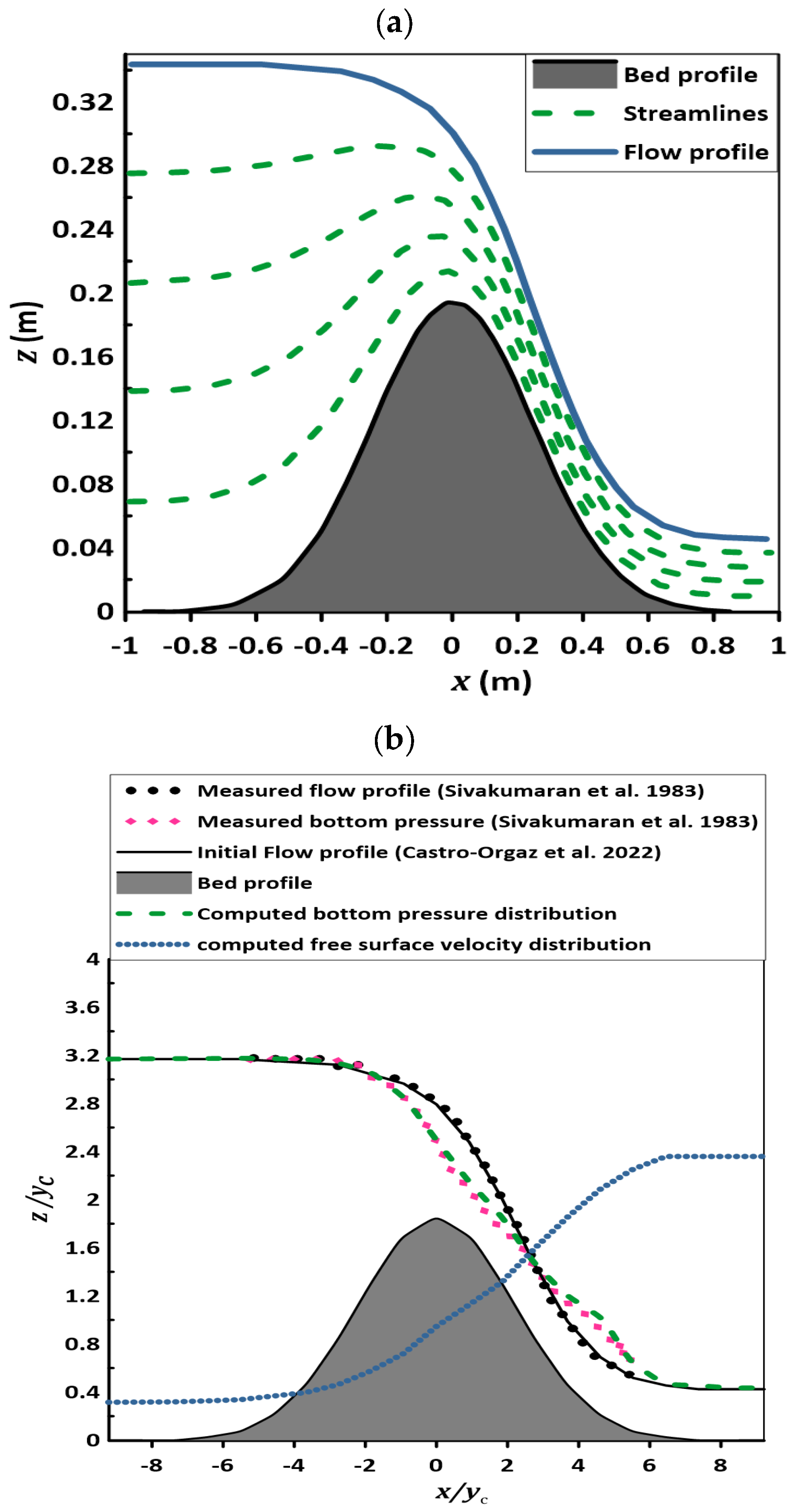
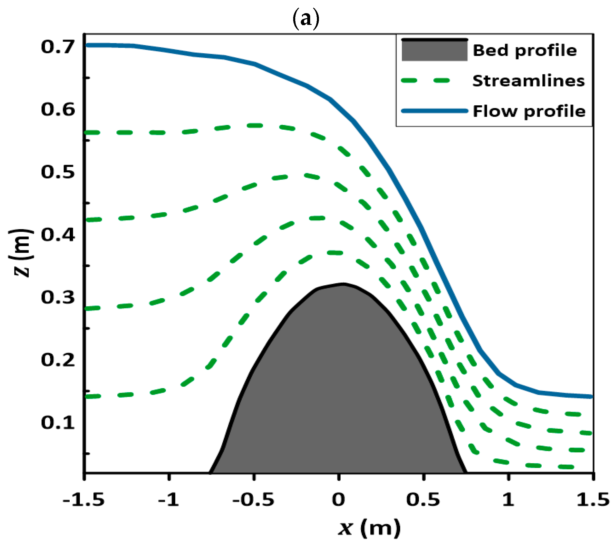
4.1. Flow over Gaussian Weir

The experimental measurements of the flow profile and bottom pressure distributions in flow over a symmetrical hump $y_b=0.2$ exp [−0.5${(x/0.24)}^2$] (m) by Sivakumaran et al. [27] are shown in Figure 3, where the potential flow model results are validated with the experimental observations. The results accord well with the experimental measurements. The discharge per unit width is 0.112 m²/s. The positions of the upstream and the downstream boundary sections are $x$(m) = ±1. In this paper, flow is modelled using 30 streamlines. The calculated pattern of streamlines is illustrated in Figure 3a, which is the solution of the semi-inverse transformation of the Laplace equation. The computed flow profile from the steady SGN equation, computed free surface velocity distribution and computed bottom pressure distributions from potential flow solutions are displayed in Figure 3b and validated with the experimental results of Sivakumaran et al. [27]. In Figure 3b, $z$ denotes the vertical coordinate, and $y_c$ denotes the critical depth. The estimated bottom pressure distribution coincides with the free surface profile close to the upstream and downstream sections, which indicates the hydrostatic pressure distribution in these regions. At the region just upstream of the weir, the streamlines have convex curvature as the flow accelerates towards the crest, leading to a decrease in bed pressure. At the crest of the weir, the radius of curvature is small, causing more pressure drop in the region. At the downstream region from $x/y_c$ = 3 to $x/y_c=6$, the streamline follows a concave path, and the radius of curvature is larger, causing the pressure rise in the region, as shown in Figure 3b. The flow surface is converging marginally at the upstream of the weir; hence, flow velocity remains constant till the crest of the weir.

The computed horizontal velocity distributions plotted at eight representative sections of the Gaussian weir are shown in Figure 4a. In the figure, $\eta$ denotes the vertical coordinate above the bed, and $U_c$ is the critical velocity. The calculated values of $u$ velocity agree well with the velocity profiles obtained from the Boussinesq approximation of Castro-Orgaz and Hager [39]. In the sections $x$ = −0.4 m to $x$ = −0.1 m, the velocity profiles are non-uniform. The $u$ velocity profile changes rapidly within the transcritical flow over the weir crest. The $u$ velocity is minimum at the surface and increases towards the bed at the crest of the weir. The shape of the velocity profile remains unchanged till $x$ = 0.2 m. At the section $x$ = 0.3 m, the velocity distribution is almost uniform in the $y$-direction. The computed vertical velocity distributions plotted at eight representative sections of the Gaussian weir are shown in Figure 4b. The calculated $v$ velocities are in good agreement with the velocity components originating from the Picard iteration [39]. The velocity profile is non-uniform with a value close to zero at the surface and increases to a positive value at the bed in the section $x$ = −0.4 m to $x$ = −0.1 m. The $v$ velocity is non-uniform at the weir crest with a value close to zero in the bed and decreases to a negative value on the surface. In the section $x$ = 0.1 m to $x$ = 0.3 m, the v velocity profile is nearly uniform with a negative value. The computed pressure distributions plotted at nine representative sections of the Gaussian weir are shown in Figure 4c. The effect of streamline curvature on pressure distribution using the Gaussian weir is observed in this study. At sections $x$ = −0.4 m to $x$ = −0.2 m, the pressure distribution is hydrostatic where the water surface coincides with the bottom pressure distributions. However, at section $x$ = −0.1 m, the pressure profile is below hydrostatic. At the crest section, the pressure profile is below hydrostatic because centrifugal acceleration induced by convex streamline curvature acts upward, opposite to gravity. In the sections $x$ = 0.1 m and $x$ = 0.2 m, the pressure profile is still below hydrostatic because of the presence of convex streamline curvature. At the section $x$ = 0.3 m, the pressure profile is just above hydrostatic. At section $x$ = 0.5 m, the pressure profile is above hydrostatic because centrifugal effects induced by concave streamline curvature act downward, in the direction of gravity.

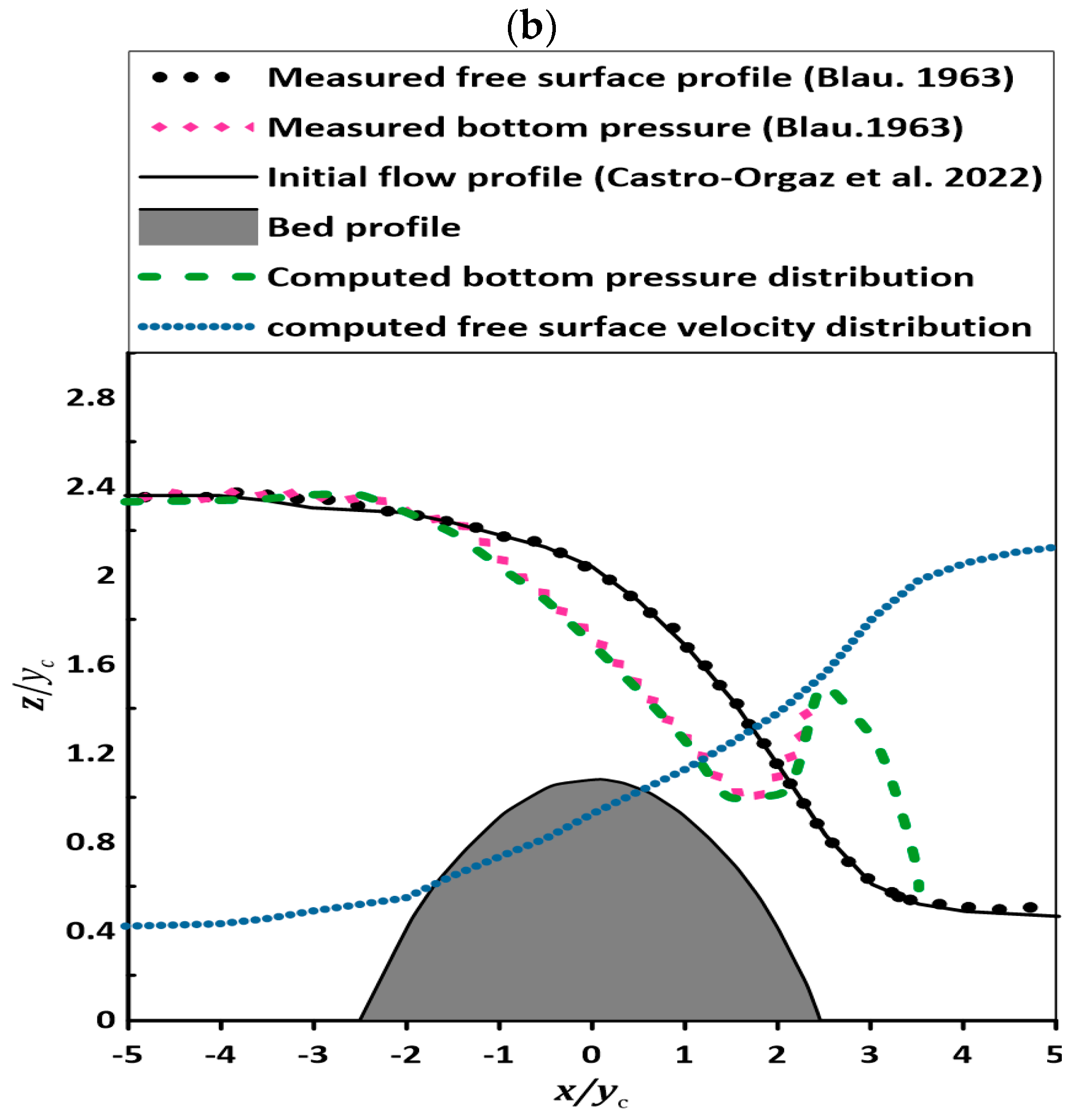
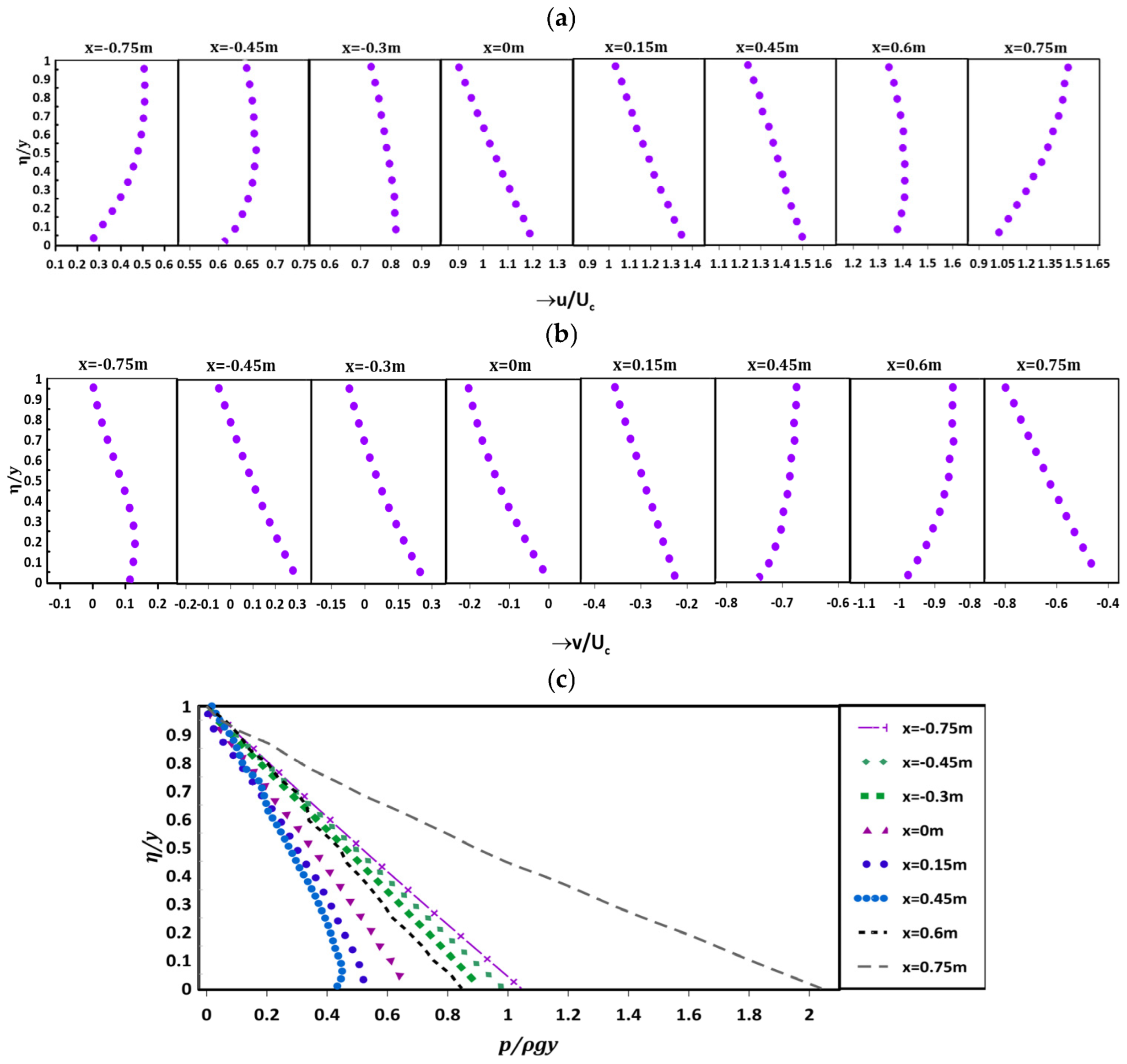
4.2. Flow over Parabolic Weir

The experimental measurements of the flow profile and bottom pressure distributions in flow over a parabolic weir $y_b=0.3216-0.54525x^2$ (m) by Blau [40] are shown in Figure 5; also, the findings of the potential flow model are validated with the measured observations, as shown in the figure. The results accord well with the experimental measurements. The discharge per unit width is 0.51 m²/s. The position of the upstream and the downstream boundary sections are $x$(m) = ±1.5. The calculated pattern of streamlines is presented in Figure 5a, which is the solution of the semi-inverse transformation of the Laplace equation. The estimated flow profile from the SGN equation, computed free surface velocity distribution and computed bottom pressure distributions from the potential flow model are displayed in Figure 5b and validated with the experimental results of Blau [40]. The bottom pressure distribution matches the free surface profile near the sections both upstream and downstream. This indicates that the hydrostatic pressure distribution is present in these areas. At the section just upstream of the weir, the streamlines exhibit a convex curvature as the flow accelerates towards the crest, leading to a decrease in the bed pressure. At the weir’s crest, where the radius of curvature is small, the pressure drop is more significant. At the downstream section, the streamline follows a concave path, and the radius of curvature is larger, causing the pressure rise in that region as shown in Figure 5b.

The computed horizontal velocity distributions plotted at eight representative sections of the parabolic weir are shown in Figure 6a. In the sections $x$ = −0.75 m and $x$ = −0.45 m, the velocity distribution is non-uniform, as shown in the figure. At the section $x$ = −0.3 m, the $u$ velocity profile tends to be constant. The streamwise velocity distribution changes rapidly within the transcritical flow over the weir’s crest. At the weir crest, the $u$ velocity is minimal at the surface and increases towards the bed. The shape of the velocity profile remains unchanged for $x$ = 0.15 m and $x$ = 0.45 m. At the section $x$ = 0.6 m, the velocity profile attains a maximum value at some distance above the bed. At the section $x$ = 0.75 m, the velocity profile varies with the maximum value at the surface and decreases towards the bed. The calculated vertical velocity distributions plotted at eight representative sections of the parabolic weir are shown in Figure 6b. At section $x$ = −0.75 m to $x$ = −0.3 m, the velocity profile is non-uniform with a value close to zero at the surface and increases to a positive value at the bed, as shown in the figure. The $v$ velocity is non-uniform from the weir crest to $x$ = 0.15 m with a value close to zero at the bed and decreases to a negative value on the surface. From the sections $x$ = 0.45 m to $x$ = 0.75 m, the $v$ velocity profile is nearly uniform with a negative value. The computed pressure distributions plotted at eight representative sections of the parabolic weir are shown in Figure 6c. The curvature of the streamlines’ influence on the vertical pressure profile is demonstrated. In the reach between $x$ = −0.75 m and $x$ = −0.45 m, the pressure profile is hydrostatic, where the water surface coincides with the bottom pressure distributions. At section $x$ = −0.3 m, the pressure distribution is just below hydrostatic. At the crest, the pressure profile is below hydrostatic because centrifugal acceleration induced by convex streamline curvature acts upward, in the opposite direction of gravity. In the sections $x$ = 0.15 m and $x$ = 0.6 m, the pressure profile is still below hydrostatic because of convex streamline curvature. At section $x$ = 0.75 m, the pressure profile is above hydrostatic because centrifugal effects induced by concave streamline curvature act downward, in the direction of gravity.

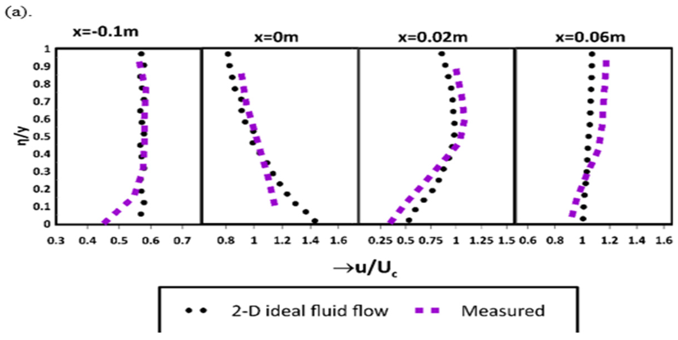
4.3. Flow over Semi-Circular Weir

The experimental measurements of the flow profiles and velocity distributions over a semicircular weir were taken in a tilting flume, set at an angle of 0.115 degrees as shown in Figure 7. The flume was 4.87 m long, 0.08 m wide, and 0.25 m high with bed and walls made of transparent Perspex. The base of the weir was attached to the flume, and the position was marked. Finally, water flow was given over the semicircular weir. The discharge per unit width is 0.022875 m²/s. The positions of the upstream and the downstream boundary sections are $x$(m) = ±0.1. The weir is located at a distance of 1.63 m from the downstream end of the flume. During the experiment, the water surface depths at respective sections are taken with the help of a point gauge. Velocity measurements are taken with the help of pitot tube arrangements. Flow is modelled using 30 streamlines. The calculated streamline flow pattern is presented in Figure 8a, which is the solution of the semi-inverse transformation of the Laplace equation. The estimated surface velocity, measured flow profile, and computed bottom pressure profiles from potential flow solutions are presented in Figure 8b. As shown in Figure 8b the pressure distribution coincides with the free surface flow, indicating the hydrostatic condition in the upstream section. The pressure drop at the weir crest is significantly greater because of strong streamline curvature. A large pressure rise is observed in the downstream section where the flow follows the concave streamline.

The computed horizontal velocity distributions plotted at four representative sections of the semicircular weir and compared with the experiments are depicted in Figure 9a. The calculated values agree well with the experimental measurements. At section $x$ = −0.1 m, the velocity distribution is non-uniform, as shown in Figure 9a. The streamwise velocity profile changes rapidly within the transcritical flow over the weir crest. At the weir crest, the $u$ velocity is minimum at the surface and increases towards the bed. At section $x$ = 0.02 m, the velocity profile changes rapidly, attaining the maximum value around mid-depth. At section $x$ = 0.06 m, the estimated velocity profile tends to be uniform; however, the velocity decreases towards the bed in the experimental measurement due to frictional resistance offered to flow by the channel boundary. The computed vertical velocity distributions plotted at four representative sections of the semicircular weir are shown in Figure 9b. At section $x$ = −0.1 m, the vertical velocity profile is uniform with a value close to zero, as shown in Figure 9b. The $v$ velocity is non-uniform at the crest of the weir with a value close to zero in the bed and decreases to a negative value on the surface. At the section $x$ = 0.02 m, the $v$ velocity profile is non-uniform with a negative value throughout the depth. At section $x$ = 0.06 m, the v velocity is non-uniform with a value close to zero at the bed and decreases to a negative value on the surface. The computed pressure distributions plotted at six representative sections of the parabolic weir are shown in Figure 9c. The influence of streamline curvature on pressure distribution is demonstrated in Figure 9c. At section $x$ = −0.1 m to $x$ = −0.02 m, the pressure profile is hydrostatic, where the free surface coincides with the bottom pressure distributions as illustrated in Figure 9c. The pressure profile is below hydrostatic at section $x$ = −0.01 m. At the crest, the pressure profile is below hydrostatic because centrifugal acceleration induced by convex streamline curvature acts upward, in the direction of gravity. At section $x$ = 0.02 m, the pressure profile is above hydrostatic because centrifugal effects caused by concave streamline curvature act downwards, in the direction of gravity.

5. Summary and Conclusions

The present study differs from the previous potential flow model by Montes [20,32] and Castro-Orgaz [22] in the following ways: (1) The present study used the Serre–Green–Naghdi equation to determine the initial water surface profile. (2) The five-point central finite difference scheme was used to discretize the partial derivative terms of the Laplace equation proposed by Boadway [19] in the interior nodes to reduce truncation errors. (3) A semicircular weir experiment was conducted to validate the pressure and velocity profiles obtained using the proposed 2-D fluid flow model.

A potential flow model of $x$-$\psi$ transformation was applied to calculate the patterns of streamlines, velocity, and pressure distributions for the selected test cases, such as Gaussian weir, parabolic weir, and semicircular weir. A steady version of the Serre–Green–Naghdi equation was used to determine the initial free-surface profile. The partial derivative terms of Laplace equations and Cartesian velocity coordinates were replaced with fourth-order accurate finite difference approximations to precisely estimate the streamline positions, thereby calculating the pressure and velocity distributions accurately. The computed flow profiles and bottom pressure distributions of Gaussian and Parabolic weirs match well with the previous experimental observations. The 2-D ideal fluid flow solution was also used to represent velocity and pressure distributions along the cross section at selected sections of all three weirs in detail. The effect of the streamline curvature on pressure distributions was observed for all three weirs discussed in the study. The rise or drop in the bed pressure depends on the nature of free surface curvature. An experiment on flow over a semicircular weir accurately predicted the shift in the velocity within the transcritical flow over the weir and the influence of the streamline curvature on pressure distributions. The computed velocity value for the semi-circular weir close to the bed slightly differed from the experimental velocity profile. Hence, the decrease in velocity near the bed was due to the boundary resistance offered to flow at the bottom.

References

1. Vo, N.D. Characteristics of Curvilinear Flow Past Circular-Crested Weir; Concordia University: Montreal, QB, Canada, 1992. [Google Scholar]
2. Vallentine, H.R. Applied Hydrodynamics; Butterworths Scientific Publications: London, UK, 1969. [Google Scholar]
3. Chanson, H. Minimum Specific Energy and Critical Flow Conditions in Open Channels. J. Irrig. Drain. Eng. 2006, 132, 498–502. [Google Scholar] [CrossRef]
4. Castro-Orgaz, O.; Chanson, H. Depth-Averaged Specific Energy in Open-Channel Flow and Analytical Solution for Critical Irrotational Flow over Weirs. J. Irrig. Drain. Eng. 2013, 140, 04013006. [Google Scholar] [CrossRef]
5. Tadayon, R.; Ramamurthy, A.S. Turbulence Modeling of Flows over Circular Spillways. J. Irrig. Drain. Eng. 2009, 135, 493–498. [Google Scholar] [CrossRef]
6. Rouse, H. Fluid Mechanics for Hydraulic Engineers; McGraw-Hill: New York, NY, USA, 1938. [Google Scholar]
7. Pu, J.H.; Huang, Y.; Shao, S.; Hussain, K. Three-Gorges Dam Fine Sediment Pollutant Transport: Turbulence SPH Model Simulation of Multi-Fluid Flows. J. Appl. Fluid Mech. 2016, 9, 1–10. [Google Scholar] [CrossRef]
8. Pu, J.H.; Cheng, N.S.; Tan, S.K.; Shao, S. Source Term Treatment of SWEs Using Surface Gradient Upwind Method. J. Hydraul. Res. 2012, 50, 145–153. [Google Scholar] [CrossRef]
9. Pu, J.H. Turbulence Modelling of Shallow Water Flows Using Kolmogorov Approach. Comput. Fluids 2015, 115, 66–74. [Google Scholar] [CrossRef]
10. Zheng, X.G.; Pu, J.H.; Chen, R.D.; Liu, X.N.; Shao, S.D. A Novel Explicit-Implicit Coupled Solution Method of SWE for Long-Term River Meandering Processinduced by Dambreak. J. Appl. Fluid Mech. 2016, 9, 2647–2660. [Google Scholar] [CrossRef]
11. Messe, P. Ressaut et Ligne D’eau Dans Les Cours à Pente Variable [Hydraulic Jump and Free Surface Profile in Channels of Variable Slope]. Rev. Gén. Hydr. 1938, 4, 7–11. [Google Scholar]
12. Andersen, V.M. Transition from Subcritical to Supercritical Flow. J. Hydraul. Res. 1975, 13, 227–238. [Google Scholar] [CrossRef]
13. Southwell, R.V.; Vaisey, G. Relaxation Methods Applied to Engineering Problems XII: Fluid Motions Characterized by Free Streamlines. Philos. Trans. R. Soc. Lond. 1946, 240, 6. [Google Scholar] [CrossRef]
14. Markland, E. Calculation of Flow at a Free Overfall by Relaxation Methods. Proc. Inst. Civ. Eng. 1965, 31, 71–78. [Google Scholar] [CrossRef]
15. Thom, A.; Apelt, C. Field Computations in Engineering and Physics; Van Nostrand: London, UK, 1961. [Google Scholar]
16. Chan, S.T.; Larock, B.E.; Herrmann, L.R. Herrmann Free Surface Ideal Fluid Flows by Finite Element Methods. J. Hydraul. Div. 1973, 99, 959–974. [Google Scholar] [CrossRef]
17. Cheng, A.H.; Liu, P.L.; Liggett, J.A. Liggett Boundary Calculations of Sluice and Spillway Flows. J. Hydraul. Div. 1981, 107, 1163–1178. [Google Scholar] [CrossRef]
18. Chow, W.L.; Han, T. Inviscid Solution for the Problem of Free Overfall. ASME J. Appl. Mech. 1979, 46, 1–5. [Google Scholar] [CrossRef]
19. Boadway, J.D. Transformation of Elliptical Partial Differential Equations for Solving Two-Dimensional Boundary Value Problems in Fluid Flow Overfall. Int. J. Numer. Methods Eng. 1976, 10, 527–533. [Google Scholar] [CrossRef]
20. Montes, J.S. A Potential Flow Solution for the Free. Proc. Inst. Civ. Eng. 1992, 96, 259–266. [Google Scholar] [CrossRef]
21. Cassidy, J.J. Irrotational Flow Over Spillways of Finite Height. J. Eng. Mech. Div. 1965, 91, 155–173. [Google Scholar] [CrossRef]
22. Castro-Orgaz, O. Potential Flow Solution for Open-Channel Flows and Weir-Crest Overflow. J. Irrig. Drain. Eng. 2013, 139, 551–559. [Google Scholar] [CrossRef]
23. Chanson, H.; Montes, J. Overflow Characteristics of Circular Weirs: Effect of Inflow Conditions. J. Irrig. Drain. Eng. 1998, 124, 152–162. [Google Scholar] [CrossRef]
24. Castro-Orgaz, O.; Hager, W.H.; Cantero-Chinchilla, F.N. Shallow Flows over Curved Beds: Application of the Serre–Green–Naghdi Theory to Weir Flow. J. Hydraul. Eng. 2022, 148, 04021053. [Google Scholar] [CrossRef]
25. Dressler, R.F. New Nonlinear Shallow-Flow Equations with Curvature. J. Hydraul. Res. 1978, 16, 205–222. [Google Scholar] [CrossRef]
26. Boussinesq, J. Essai Sur La Theorie Des Eaux Courantes; Memoires Presentes Par Divers Savants a l’Academie Des Sciences; Imprimerie Nationale: Paris, France, 1877; pp. 1–680. Available online: https://gallica.bnf.fr/ark:/12148/bpt6k56673076 (accessed on 11 August 2024).
27. Sivakumaran, N.S.; Tingsanchali, T.; Hosking, R.J. Steady Shallow Flow over Curved Beds. J. Fluid Mech. 1983, 127, 469–487. [Google Scholar] [CrossRef]
28. Naghdi, P.M.; Vongsarnpigoon, L. The Downstream Flow beyond an Obstacle. J. Fluid Mech 1986, 162, 223–236. [Google Scholar] [CrossRef]
29. Matthew, G.D. Higher Order, One-Dimensional Equations of Potential Flow in Open Channels. Proc.—Inst. Civ. Eng. Part 2 Res. Theory 1991, 91, 187–201. [Google Scholar] [CrossRef]
30. Zhu, D.Z.; Lawrence, G.A. Non-Hydrostatic Effects in Layered Shallow Water Flows. J. Fluid Mech. 1998, 355, 1–16. [Google Scholar] [CrossRef]
31. Castro-Orgaz, O.; Cantero-Chinchilla, F.N. Non-Linear Shallow Water Flow Modelling over Topography with Depth-Averaged Potential Equations; Springer: Amsterdam, The Netherlands, 2020; Volume 20, ISBN 0123456789. [Google Scholar]
32. Montes, J.S. Potential-Flow Solution to 2D Transition from Mild to Steep Slope. J. Hydraul. Eng. 1994, 120, 601–621. [Google Scholar] [CrossRef]
33. Wei, G.; Kirby, J.T.; Grilli, S.T.; Subramanya, R. A Fully Nonlinear Boussinesq Model for Surface Waves. Part 1. Highly Nonlinear Unsteady Waves. J. Fluid Mech. 1995, 294, 71–92. [Google Scholar] [CrossRef]
34. Brocchini, M. A Reasoned Overview on Boussinesq-Type Models: The Interplay between Physics, Mathematics and Numerics. Proc. R. Soc. A Math. Phys. Eng. Sci. 2013, 469, 20130496. [Google Scholar] [CrossRef] [PubMed]
35. Hosoda, T. Akhide Tada Free Surface Profile Analysis of Open Channel Flows by Means of 1-D Basic Equations with Effect of Vertical Acceleration. Proc. Hydraul. Eng. 1994, 38, 457–462. [Google Scholar] [CrossRef]
36. Onda, S.; Hosoda, T. Numerical Simulation on Development Process of Dunes and Flow Resistance. Proc. Hydraul. Eng. 2004, 48, 973–978. [Google Scholar] [CrossRef]
37. Komai, Y. Basic Characteristics on the Response of Water Surface Profiles of Open Channel Flows over an Obstacle. Bachelor’s Thesis, Undergraduate School of Kyoto University, Kyoto, Japan, 2006. [Google Scholar]
38. Abramowitz, M.; Stegun, I.A. Handbook of Mathematical Functions with Formulas, Graphs, and Mathematical Tables, 10th ed.; Wiley: New York, NY, USA, 1972. [Google Scholar]
39. Castro-Orgaz, O.; Hager, W.H. Velocity Profile Approximations for Two-Dimensional Potential Open Channel Flow. J. Hydraul. Res. 2013, 51, 645–655. [Google Scholar] [CrossRef]
40. Blau, E. Der Abfluss Und Die Hydraulische Energieverteilung Über Einer Parabelförmigen Wehrschwelle (Distributions of Discharge and Energy over a Parabolic-Shaped Weir); Mitteilungen der Forschungsanstalt für Schiffahrt, Wasser- und Grundbau: Berlin, Germany, 1963. [Google Scholar]
Figure 1. Potential flow definition sketch in the x - y plane for (a) Gaussian weir; (b) parabolic weir; (c) semicircular weir. (d) Potential flow in x - ψ plane subdivided in finite difference grid.
Fluids 09 00182 g001
Figure 2. Notations for indicating the position of streamlines of adjacent nodes in the array.
Fluids 09 00182 g002
Figure 3. Flow over Gaussian weir of Sivakumaran et al. [27]. (a) Computed streamlines. (b) Computed flow profile [24], surface velocity and bottom-pressure distributions, validated with experimental measurements.
Fluids 09 00182 g003
Figure 4. Flow features along the Gaussian weir domain computed with 2D fluid flow solution and validated with the results of Castro-Orgaz and Hager [39]: (a) horizontal velocity distributions; (b) vertical velocity distributions; (c) pressure distributions.
Fluids 09 00182 g004
Figure 5. Flow over parabolic weir of Blau [40]. (a) Computed streamlines; (b) computed flow profile [24], surface velocity and bottom-pressure distributions, validated with experimental measurements.
Fluids 09 00182 g005aFluids 09 00182 g005b
Figure 6. Flow features along the parabolic weir domain computed with 2D fluid flow solution: (a) horizontal velocity distributions; (b) vertical velocity distributions; (c) pressure distributions.
Fluids 09 00182 g006
Figure 7. (a) Schematic layout of the experimental setup. (b) Hydraulic flume with point gauge and pitot tube arrangements. (c) The semicircular weir in the experiment. (d) Pitot tube arrangements for velocity readings.
Fluids 09 00182 g007
Figure 8. Flow over semi-circular weir: (a) Computed streamlines; (b) Computed flow surface velocity and bottom-pressure distributions, validated with experimental measurements.
Fluids 09 00182 g008
Figure 9. Flow features along the semi-circular weir domain computed with 2D fluid flow solution and compared with experimental measurements: (a) horizontal velocity distributions; (b) vertical velocity distributions; (c) pressure distributions.
Fluids 09 00182 g009aFluids 09 00182 g009b
Disclaimer/Publisher’s Note: The statements, opinions and data contained in all publications are solely those of the individual author(s) and contributor(s) and not of MDPI and/or the editor(s). MDPI and/or the editor(s) disclaim responsibility for any injury to people or property resulting from any ideas, methods, instructions or products referred to in the content.