Abstract
Computational fluid dynamics (CFD) is a numerical tool often used to predict anticipated observations using only the physics involved by numerically solving the conservation equations for energy, momentum, and continuity. These governing equations have been around for more than one hundred years, but only limited analytical solutions exist for specific geometries and conditions. CFD provides a numerical solution to these governing equations, and several commercial software and shareware versions exist that provide numerical solutions for customized geometries requiring solutions. Often, experiments are cost prohibitive and/or time consuming, or cannot even be performed, such as the explosion of a chemical plant, downwind air concentrations and the impact on residents and animals, contamination in a river from a point source loading following a train derailment, etc. A modern solution to these problems is the use of CFD to digitally evaluate the output for a given scenario. This paper discusses the use of CFD at Corteva and offers a flavor of the types of problems that can be solved in agricultural manufacturing for pesticides and environmental scenarios in which pesticides are used. Only a handful of examples are provided, but there is a near semi-infinite number of future possibilities to consider.
1. Introduction
Engineering principles have traditionally been divided between experimental and theoretical disciplines, with the former being dominated at agrochemical companies such as Corteva, Syngenta, BASF, and FMC. Experiments are often considered and required by regulatory bodies to understand objective details, but these experiments are often expensive, risky, and time consuming. Modeling and simulations based upon science, math, and computer science began in the 1950s and their use has been increasing recently due to the rapid evolvement of CPUs. Even today’s computer desktops/laptops, running more than a single CPU (multi-processers), would have been classified as supercomputers several decades ago (a supercomputer can be thought of as a machine/server with multiple CPUs grouped into tens to thousands of computing nodes). This is often convenient for solving real-world problems that can be easily solved by theory vs. often expensive experimental analysis.
Computational Fluid Dynamics (CFD) is a modeling and simulation technique based upon fluid flow modeling and has been around for the past 50 years, providing a numerical solution to the governing equations of conservation of mass, momentum, and energy (Equations (1)–(3)). These governing conservation equations (e.g., theories) are solved numerically using various techniques such as Large Eddy simulation [1,2,3,4,5,6] and can offer insight when no experimental knowledge is available or is difficult to measure (i.e., discrete element modeling, finite difference, volume of fluid (VOF) method, etc.). Today’s CPU horsepower has been used to solve complex problems that were difficult to solve only a decade ago. Thus, problems involving fluid flow, heat and mass transfer, reactive flow, multi-phase flow and combustion can now be simulated via various computational models. Some real-world examples of CFD use include multiphase flow (e.g., the breakup of formulations being sprayed in air, waves breaking on a beach, etc.), the design of airplanes/cars where drag can influence design, etc. CFD is often used when experiments are costly or cannot be carried out (i.e., experiments on humans, catastrophic events like sabotage to chemical facilities, manufacturing where changes in input conditions often are limited w/o interrupting production, and so on). In the EU and USEPA, even low mammal toxicity testing is coming under fire, so a future without any animal testing can be achieved (EPA by 2035, and the EU already banned testing for cosmetics in 2013). CFD is an ideal pathway used to simulate these results without the need for human and animal testing.
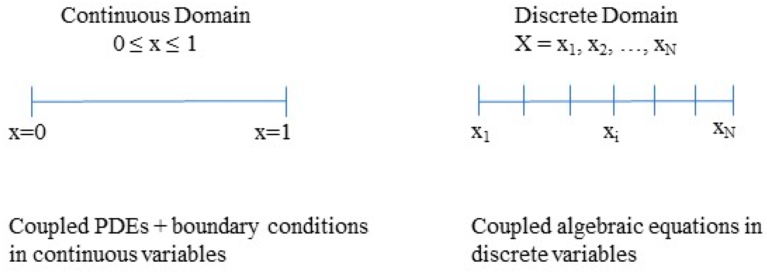
CFD replaces the continuous problem domain with a discrete domain using a grid. Thus, numerical methods are used to convert these partial differential governing equations to a coupled algebraic set of equations. Typically, the governing partial differential equations of fluid mechanics are first discretized into algebraic equations using specialist numerical techniques/methods such as Finite Differences, Finite Elements, Finite Volumes, Lattice Boltzmann, Smoothed Particle Hydrodynamics, etc. Specialist matrix solvers which can be both iterative (i.e., Conjugate Gradient) or direct (Multi-Frontal) are then used to solve this algebraic system of equations. Each variable is defined at every point in the continuous domain, while in the discrete domain, each variable is defined only at the grid points, as in Figure 1. CFD directly solves for flow variables only at the grid points, but interpolation techniques are used for values between the grid points. The discrete variables become a large system of coupled algebraic equations that involves iterative calculations amenable for computer computation. The reader can view many introductory writings on CFD found elsewhere [7,8,9,10,11,12,13,14]. Solving CFD problems involves three major steps that include (i) preprocessing (creation of geometry and meshing), (ii) solving the governing equations over this meshed model, and (iii) post-processing results to be analyzed. An example is defined at every point in the continuous domain converted into a discrete domain.
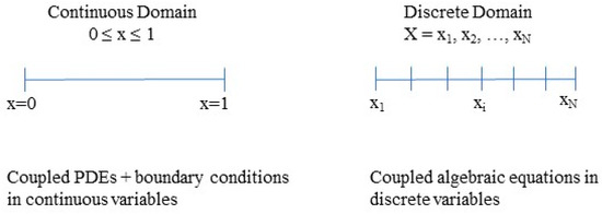
Figure 1.
Example continuous to discrete domain in 1 dimension (i.e., discretizing).
2. Materials and Methods
Conservation of mass can be expressed as
C = Concentration;
D = Diffusion coefficient;
u = Velocity vector.
The conservation of momentum equation can be written as
where (1) represents inertial forces, (2) pressure forces, (3) viscous forces, and (4) external forces applied to the fluid (i.e., gravity).
μ = viscosity;
V = kinematic viscosity = μ/ρ;
u = V = velocity vector;
ρ = fluid density;
I = identity matrix;
F = body force term;
p = pressure;
T = temperature;
τ = shear stress tensor;
D/Dt = material derivative (the rate of change following a moving fluid parcel);
k = material thermal conductivity;
et = Cv T + u2/2 = specific internal energy (internal energy per unit mass);
fG = external body forces acting on the fluid (such as gravity);
Sg = generation source term for energy (radiation effects, thermal heating from electrical current, etc.).
The conservation of energy can be written as
and is used to generate temperatures for the scenario being investigated. Each term in the continuity, momentum, and energy equation (e.g., Equations (1)–(3)) can be found in any elementary treatise on the subject (Bird, Stewart, Lightfoot, 1960 [15]). All three governing equations are numerically solved to generate solutions using CFD. There are many opensource (free) CFD packages, such as OpenFOAM, SU2, Palabos, Fire Dynamics Simulator, and MFIX (OpenFOAM is most popular with users, with a tutorial, extended code, and programmers guide), along with many commercial packages users can utilize. A major advantage of commercial CFD packages is the ease of use via graphical user interfaces for pre- and post-processing, which reduces the hurdle associated with learning the package. CFD code became common during the 1950s–1970s. Computers necessary to run such code cost ~USD 10 million (2024 dollars) and key players were the Los Alamos National Lab, Douglas Aircraft, and NASA, with code written to model specific (not generic) examples. Off-the-shelf commercial code become available during the 1980s–2010s, and many examples of this work used the commercial CFD package COMSOL Multiphysics (https://www.comsol.com, accessed on 11 August 2024), but other packages exist, such as ANSYS FLUENT (https://www.ansys.com, accessed on 11 August 2024), STAR-CCM+ (https://plm.sw.siemens.com/en-US/, accessed on 11 August 2024), Altair (https://www.altair.com/altair-cfd, accessed on 11 August 2024), etc. These codes are designed to run on CPUs and often require extensive training and project time (weeks/months) and computers to run this software, costing ~USD 1–10 million (in 2024 dollars). More recently, GBU execution has evolved (2010s–present) and can be orders of magnitude faster than CPU code via software such as MstarCFD (https://mstarcfd.com accessed on 11 August 2024), Palabos (University of Geneva, https://palabos.unige.ch/publications/ accessed on 11 August 2024), and LB-2D (Harvard University, Randles and Kaxiras 2014 [16]). Project time is now measured in hours or days using computers costing ~USD $2000 (in 2024 dollars). Examples of various GBU algorithms are found in Figure 2.
𝜕 (ρ et)/𝜕t + ∇∙u (ρ et + p) = ∇∙[k ∇T + τ∙u] + Sg
Figure 2.
Examples of various GBU approaches in use. 1 https://www.sciencedirect.com/science/article/pii/S0898122111001064 (accessed on 11 August 2024), 2 https://www.sciencedirect.com/science/article/abs/pii/S092702561930206X (accessed on 11 August 2024), 3 https://papers.ssrn.com/sol3/papers.cfm?abstract_id=4368195 (accessed on 11 August 2024), 4 https://onlinelibrary.wiley.com/doi/abs/10.1002/num.22730 (accessed on 11 August 2024).
3. Results
What follows are specific R&D examples where CFD has been used at Corteva to offer the reader a flavor for the types of simulations and results that can be obtained. This section is broken into two parts, namely (1) General Corteva R&D Examples, and (2) Corteva Manufacturing Examples. It takes an agrochemical company approximately USD 250–300 million and over 10 years of studies to obtain registration of an active ingredient for commercial use. CFD is often used to “fill-in” our understanding of the manufacturing process and environmental fate of a molecule once placed in the environment. The examples provided illustrate the importance of CFD in both R&D and manufacturing at Corteva, and in many cases deal with predictions that could not be measured directly (e.g., testing on humans) or were cost-prohibitive to achieve.
3.1. General Corteva R&D Examples
3.1.1. Potential for Breathing in a Volatile Pesticide
We begin with an R&D example to understand the propensity for humans to breathe in and intake volatile/semi-volatile pesticides. A soil fumigant is a pesticide that when applied to soil forms a gas that subsequently emanates within the soil pores to control pests that ultimately impact crop production and yield. The soil fumigant 1,3-dichloropropene (1,3-D), sulfuryl fluoride (used to treat buildings and grain storage areas), and various metabolites of active pesticides (e.g., IN-VM862, a soil metabolite of Reklemel) are all examples of volatile pesticides. Semi-volatile pesticides include chlorpyrifos, various formulations of 2,4-D, dicamba, etc. The volatile soil fumigant 1,3-dichloropropene (1,3-D) used to be a USD 150 MM a year product for Dow AgroSciences, but went back to the Dow Chemical portfolio following the creation of Corteva in 2019. However, the following example highlights the power of CFD when experiments on humans could not be performed. 1,3-dicloropropene is injected into the ground as a liquid to control nematodes (primarily) and some weed species. The material vaporizes and begins to rise back towards the soil surface, while impacting soil-borne nematodes. There are several techniques to stop the material at the soil surface, such as the use of tarps or some types of chemical and/or an impermeable layer, but the potential of becoming airborne is a real possibility and thus can create potential inhalation risks for humans.
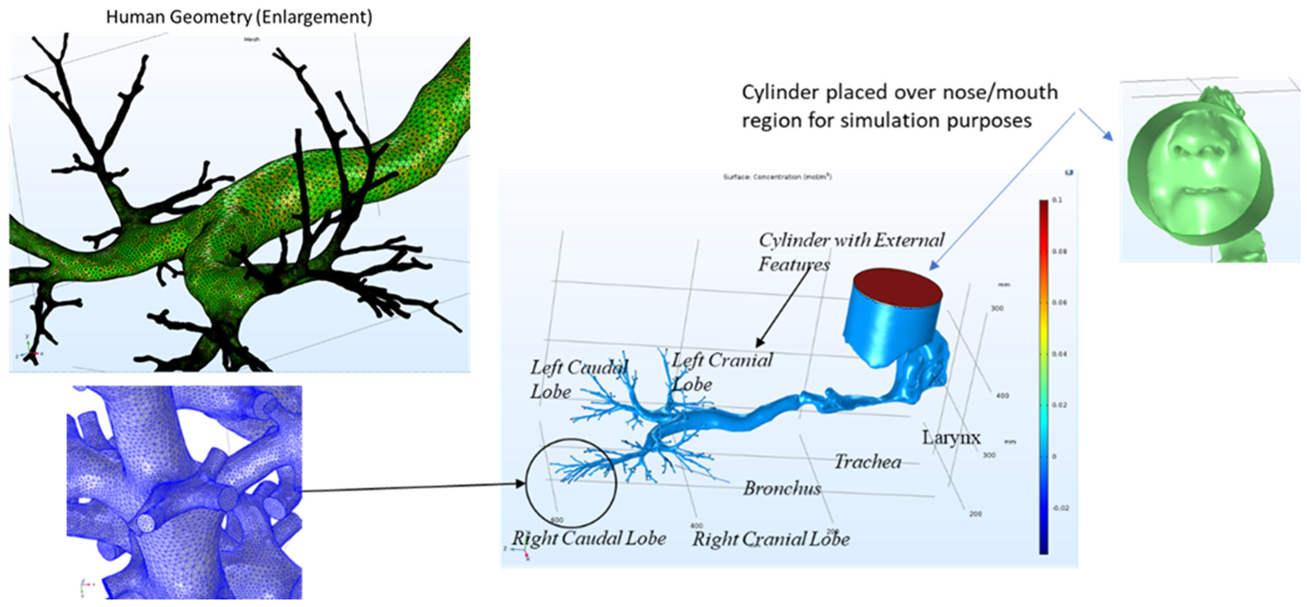
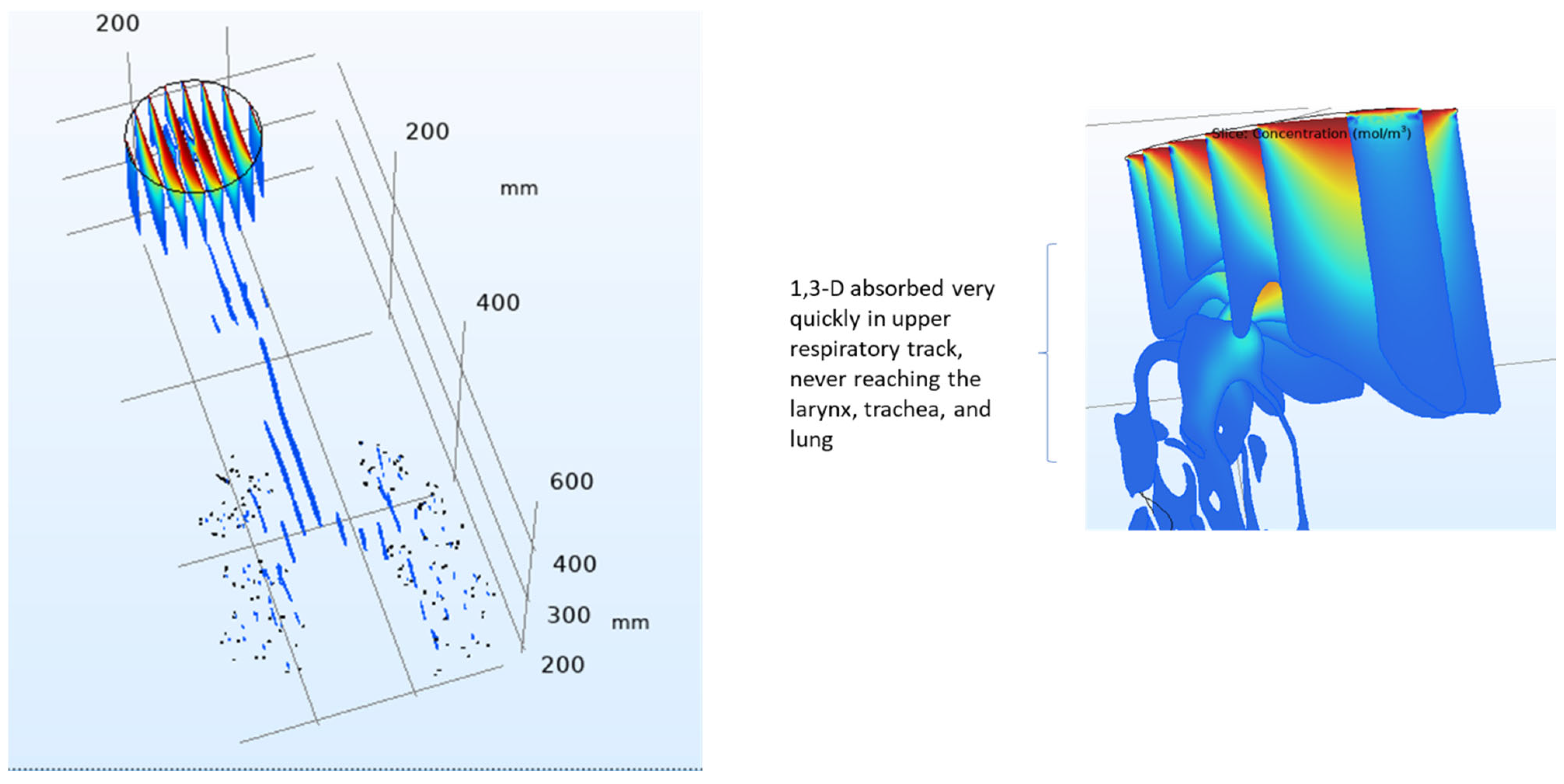
References for three dimensional CFD modeling for inhaled material transport are found elsewhere [17,18,19,20]. The following provides an example of the use of CFD for 1,3-D, which was undertaken about the time the product was returned to Dow when Corteva was formed. It is based upon an award-winning paper by Corley et al., 2012 [21] (Pacific Northwest National Lab). These researchers investigated the inhalation of a volatile material when smoking cigarettes. Files used by Corley et al., 2012 [21] were converted from OpenFoam (a freeware CFD package) to COMSOL Multiphysics. Now, we assume that a former Corteva product (1,3-dichloropropene) resulting from agricultural use was inhaled instead of cigarette smoke. COMSOL was used for human and rat inhalation scenarios; see Figure 3 and Figure 4. This analysis bypassed the need for lower tier (and higher safety factor) approaches and allowed Corteva to assess the risk directly associated with inhaled vapor of 1,3-dichloropropene. Computed tomography (CAT) scans for a human and rat (corpses) were used, with a cylinder placed around the mouth/nose for CFD input; see Figure 3. The assigned breathing rates for a typical human and rat were used, partition coefficients and physicochemical properties for 1,3-D, etc., were assumed, and the determination of where 1,3-D was absorbed in the body was determined. The regional uptakes of 1,3-D in the human respiratory track were sensitive to air concentration levels, airflow rates, air-tissue partition coefficients, tissue thickness, and metabolism rates and occurred early in the process, well before reaching the lung. CFD predictions of 1,3-D exposure and uptake to humans via the inhalation exposure route eliminated the simplistic back-of-the-envelope exposure approaches (with safety factors) often used to estimate dose and exposures for inhalation gas dosimetry, while providing a key scientific approach for the inhalation dosimetry of gasses. It was found that 1,3-D is absorbed rapidly early in the breathing process (e.g., in the trachea) and does not reach deep into the lungs when predicted losses of 1,3-D from the soil (vapor phase) are anticipated; see Figure 4. Computational Fluid Dynamics eliminates the need for lower-tier (and higher safety factor) approaches to allow the ability to predict risk associated with inhaled vapor and aerosol exposures of organic chemicals.

Figure 3.
Example of using CFD modeling when experiments cannot be performed (human/rat breathing 1,3-D-laden air required for reregistration of 1,3-D).

Figure 4.
COMSOL CFD results [human, 1,3-D concentration results (mol/m3)].
3.1.2. Reactor Design
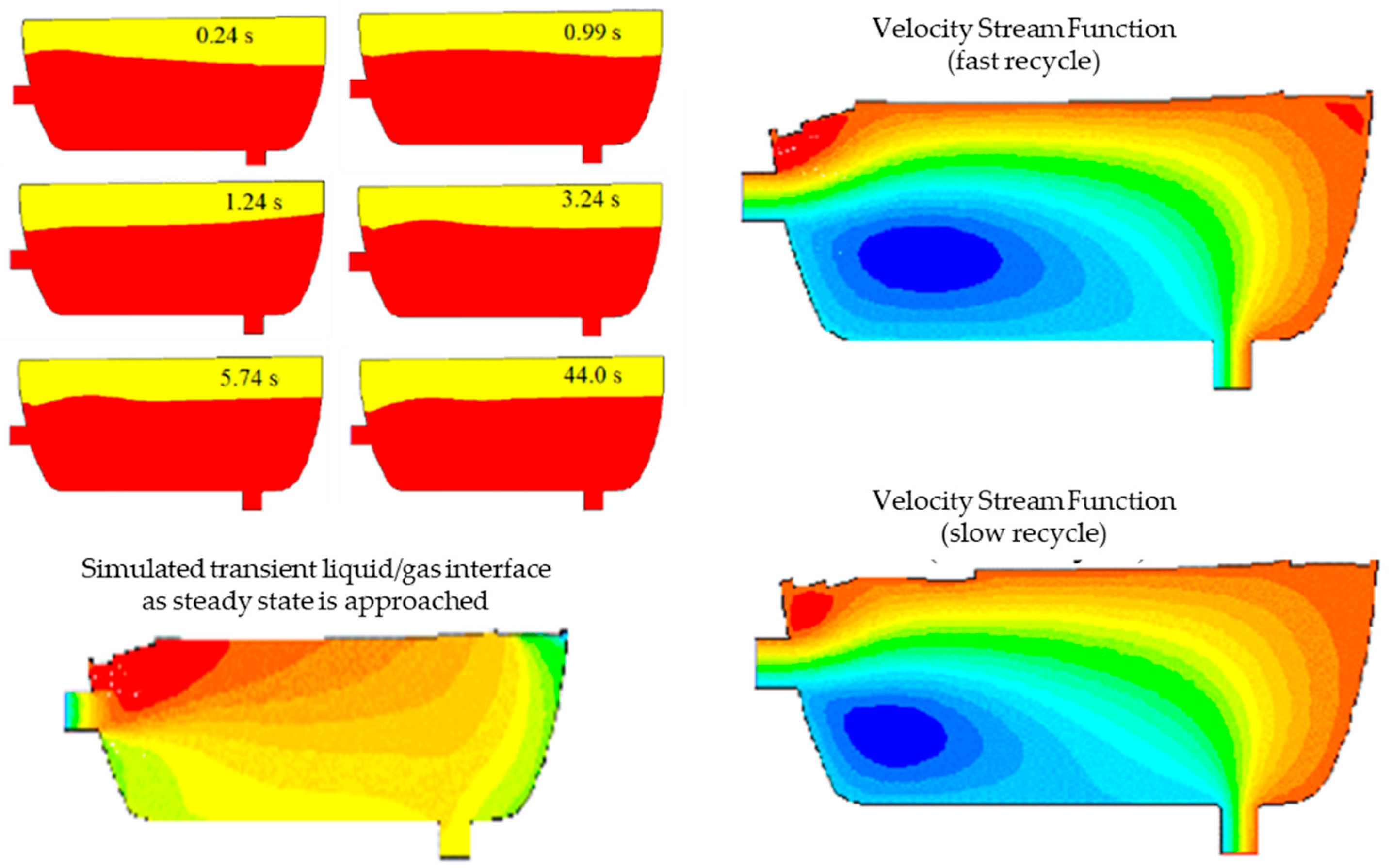
Several decades ago, CFD was used to investigate whether process conditions for the dichlorophenol reactor in Midland, MI (a precursor to 2,4-D synthesis) could be operated to enhance dichlorophenol yield. Several findings from this work summarized the filling of the reactor with fluid, the simulation of the transient liquid/gas interface as a steady state was considered, and operating conditions were looked at for the recycle stream as a product to be recycled back into the reactor to optimize performance; see Figure 5. As the velocity stream is slowed (slow recycle), the recycle region within the reactor is minimized, thus giving insight into the ideal conditions for operating the reactor.

Figure 5.
CFD results using the FLUENT software package to simulate the optimal practices for filling and operating the dichlorophenol reactor.
3.1.3. Home Fumigation
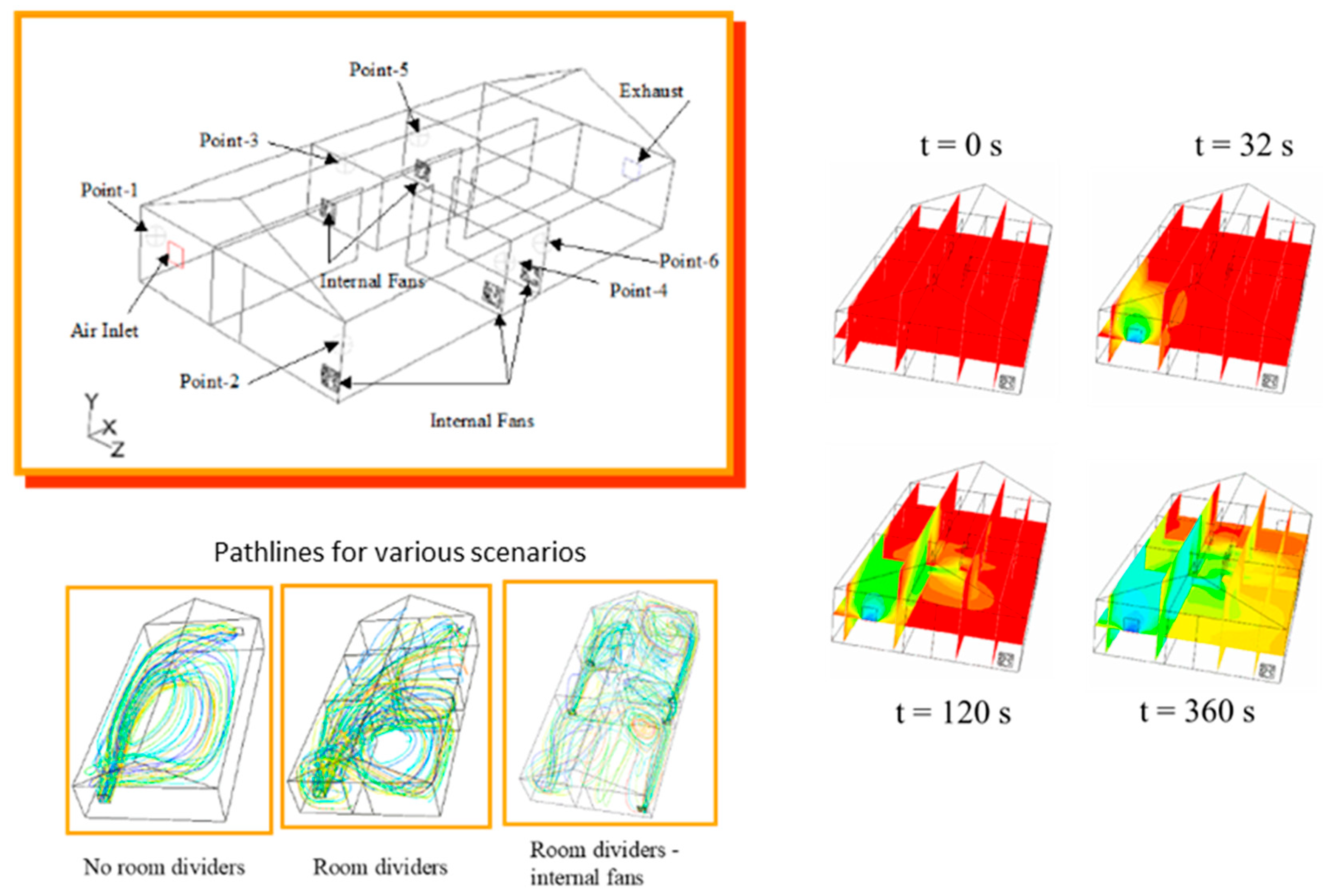
Sulfuryl fluoride is a gas that is pumped into a house/structure for around a 24 h period to kill insect pests. The structure is often covered with tarps during fumigation to keep the fumigant from leaking out. Following fumigation, the structure is vented to the outside using fans, open doors/windows, etc., so residents and workers can reenter safely. Several constraints need to be heeded. First is that the venting to the outside is slow enough that the outside air concentrations are below threshold levels for the safety of residents/passersby in proximity, and the second deals with when residents can safely return to the structure post fumigation and ventilation. CFD is an ideal tool to address this scenario; see Figure 6.
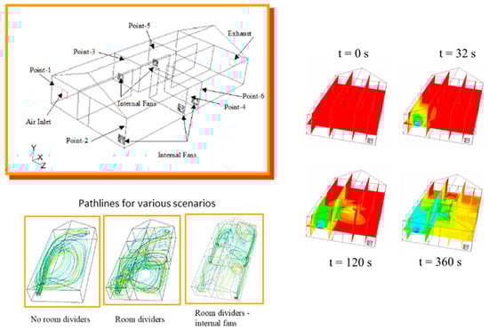
Figure 6.
Home aeration following pest fumigation (e.g., when can a resident safely reenter a treated structure?) Graphic on the right gives 2D slices in the 3D simulation domain as the home is aerated with fresh air.
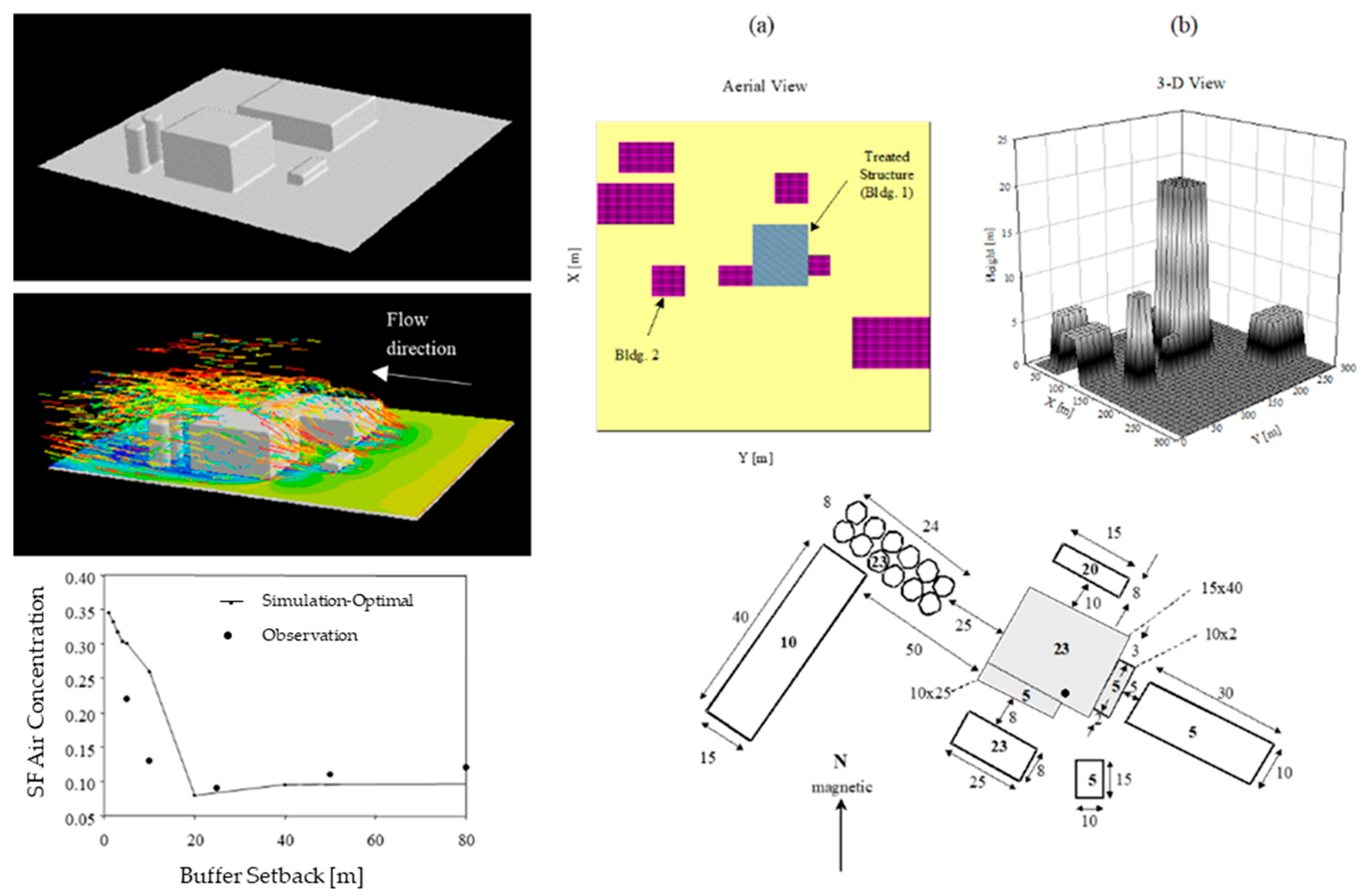
Outside air concentrations were simulated following mill fumigation using Sulfuryl Fluoride, where the gas was released into the environment; see Figure 7. Best management practices could be deciphered to minimize bystander exposure during the clearing process for the mills, such that operators could safely return [22,23]. The work documented in this Biosystems Engineering paper, “Estimating Outside Air Concentrations Surrounding Fumigated Grain Mills,” won the EurAgEng outstanding paper award from Biosystems Engineering in 2008, the only nonacademic paper to do so [24].

Figure 7.
Mill fumigation and aeriation with potential exposure to sulfuryl fluoride, with results compared to experimental results for different large-scale milling facilities. (a) Aerial View, (b) 3-D View.
3.1.4. Quantifying Efficacy and Bystander Exposure from Expanded Uses of Sulfuryl Fluoride
Grain is often stored on the ground and covered with a tarp for extended periods of time before being taking to market in regions such as Australia and New Zealand. A fumigant such as sulfuryl fluoride is often used to control pests over this time interval. An applicator walks along the tarp and injects fumigant into the grain below and repeats this process until the entire pile has been treated. CFD was used to simulate the resulting concentration profile in the grain as a function of depth and location, such that advice about application practices (and amount of chemical used) can be made to maximize efficacy; see Figure 8.
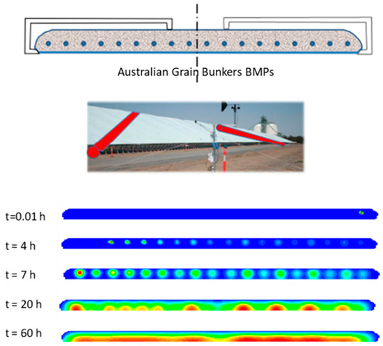
Figure 8.
An Australian grain bunker treated with sulfuryl fluoride to control insect pests, where CFD was used to simulate the amount, location, and duration (e.g., best management practices (BMP)) for the pesticide such that efficacy estimates could be made.
3.1.5. Drift Loading to Stream and Backwater Regions: Refinement of Acute Exposure
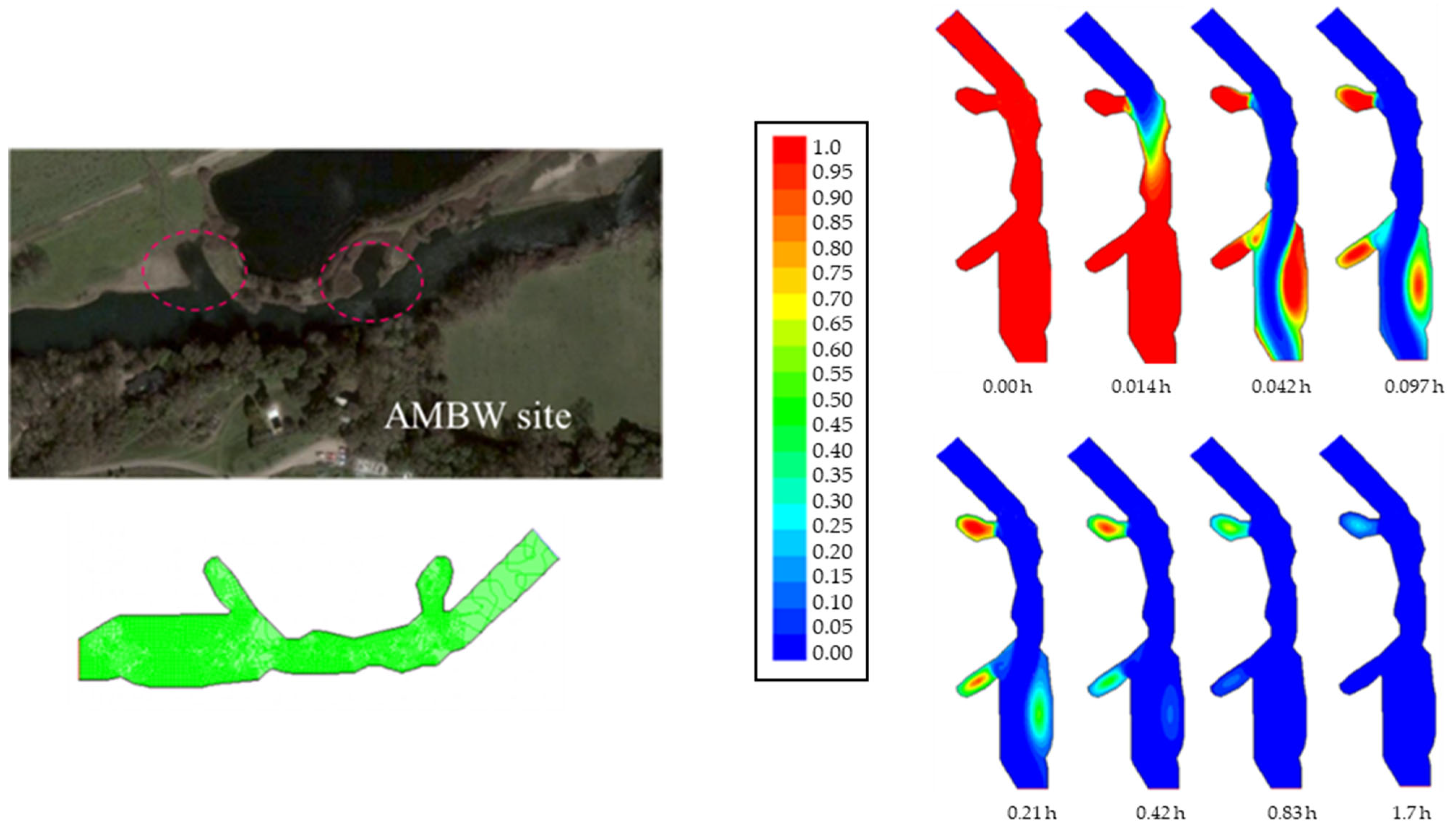
Salmon are an endangered species in California, USA. In many areas of California, agricultural fields often border streams where small salmon live during part of their lifecycle, before heading back to the ocean to grow, ultimately returning to these streams to spawn and continue this lifecycle. There is a concern that pesticide sprays from neighboring farms can enter these surface waters and injure the small salmon fry that live there. This work looked at three different regions within the Mokelumne River that have backwater regions where these young salmon fry live. Thus, work was undertaken to see if a stream received pesticide loading from a spray drift, and then to see how long the concentrations remained in the stream, especially in these backwater regions where the salmon live. CFD was an ideal tool to simulate the residence time in this California stream for a pesticide to be cleared following the original insult; see Figure 9. These transient concentrations could be compared with acute toxicity data for the organism in question.
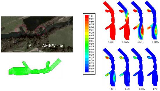
Figure 9.
Drift loading to stream and backwater regions: 2D geometry of the stream section was discretized by hand, where backwater regions are clearly seen. Graphic on the right is the transient stream mass fraction following a chemical insult predicted by CFD.
3.1.6. Predicting Pesticide Volatility through Coupled above/below Ground Multiphysics Modeling
A large CFD simulation that involves both mass transfer for chlorpyrifos (semi-volatile) from plant surfaces and chlorpyrifos air concentrations once in the air was conducted, such that volatile airborne concentrations of chlorpyrifos could be addressed. The flow field and streamlines for geometries associated with row/furrow agriculture for a peach tree are found in Figure 10 (tree only). The air velocity is much lower near the plant/crop due to the crop canopy, due to obstructions created by the plant (Figure 10). The highly curved streamlines (Figure 10) lead to effective mixing of pesticide vapor within the canopy. Interested readers can find more detail elsewhere (Mao et al., 2018 [25], Wolters et al., 2004 [26]; Yates et al., 2002 [27]).
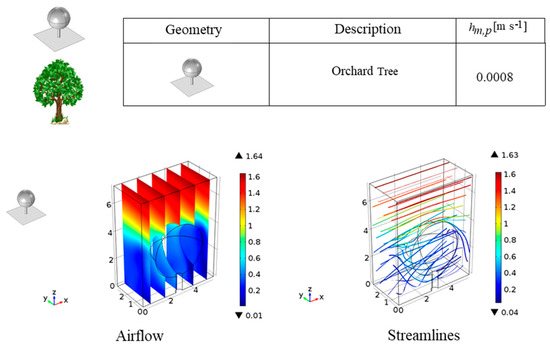
Figure 10.
Turbulent flow past a modeled tree (top); air flow (left) and airflow streamlines (right). Specific details can be found in Mao et al., 2018 [25].
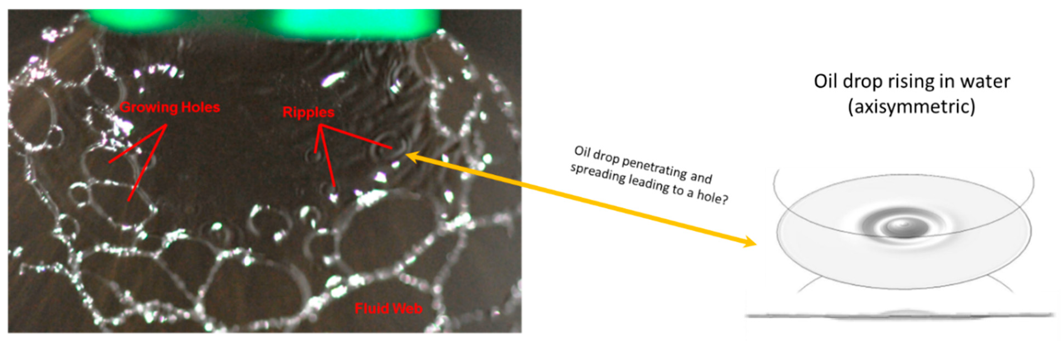
3.1.7. Why Holes Form in Oil-in-Water-Sprayed Liquid Sheets, Leading to Sheet Breakup
The breakup for a spray sheet consisting of an oil-in-water formation (e.g., atomization of a continuous sheet emanating from an agricultural spray nozzle) was also investigated using CFD. The breakup pattern for oil-in-water formulation starts with holes first forming within the spray sheet. These holes grow, collide, and eventually lead to sheet breakup. The oil drop within the water makes it way to the air/water interface and creates a disturbance; see Figure 11. These disturbances can grow and lead to holes within the sheet that are responsible for the sheet’s demise and the resulting atomization drop sizes that ensue. Details of the modeling approaches for oil-in-water formulation breakup patterns emanating from agricultural nozzles mounted along a spray boom can be found elsewhere (Altieri et al., 2014 [28], Cryer and Altieri, 2017 [29], Altieri and Cryer, 2018 [30], Krishnan et al., 2022 [31].
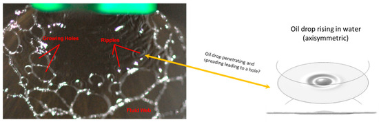
Figure 11.
CFD results for the “dimple” that that forms in an oil-in-water formulation being sprayed from an agricultural nozzle as an oil drop penetrates the water film surface, compared to an observation of the film breakup process.
3.2. Corteva Manufacturing Examples
As discussed in the introduction section, CFD involves the use of computer modeling to study a system or process equipment to visualize the fundamental fluid flow-based physics associated with the chemical process. The biggest advantage of using CFD modeling in manufacturing is that it does not rely on any scale-up or scale-down approaches, due to its reliability on fundamental governing equations of fluid flow (i.e., mass, momentum, and energy balances).
Additional benefits of using CFD in manufacturing are listed below:
- Achieving a better understanding of the physical phenomena in mixing-based processes.
- Prototyping mixing designs at manufacturing scale cost-effectively compared to experiments.
- Evaluating impacts of design/parameter changes through computer simulations.
- Understanding transient effects and mixing heterogeneities during scale-up.
CFD can be generically used for
- Troubleshooting and hypothesis testing;
- Feasibility studies;
- Engineering design, redesign, and optimization;
- Flow-physics-based visualization.
The traditional approach to characterizing mixing and associated physics, mass transfer, and chemical reactions in mixing systems has been to apply engineering correlations based on a combination of first principles and empirical relationships. This is a logical first step to understanding a mixing process. The investment is low, and the information is quite useful. Furthermore, the process of gathering the specific information necessary for this approach is essential for understanding the process. However, the challenge for the mixing experts is to navigate the vast amount of literature that is typically written for specific systems and then apply it to their unique mixing process.
Our present computational methodology to model, simulate, and understand mixing-based multi-physics processes within Corteva includes using a Lattice Boltzmann LES framework on GPU architecture [32,33,34]. This strategy inherently alleviates the limitations posed by Reynolds Averaged Navier–Stokes (RANS)-equation-based approaches by resolving the transients in fluid flow, turbulence, and additional physics associated with scalar species transport, gas–solid, gas–liquid mass transfer, liquid–liquid immiscible interactions, non-Newtonian rheology, bubble coalescence/break-up, bubble/particle motion tracking, and rotating impeller/shaft geometries within the stirred tank reactor vessels or continuous flow reactor systems.
Corteva in-house applications of CFD in manufacturing (specifically related to mixing) include:
- Flows in batch and continuous processes.
- Mixing and mass transfer in stirred tank reactors;
- ○
- Mixing/blend time calculations;
- ○
- Power requirement calculations;
- ○
- Vortexing and splashing computations;
- ○
- Non-Newtonian fluid mixing;
- ○
- Multiple miscible fluid blending;
- ○
- Gas–liquid mixing and mass transfer.
- Flow in static/in-line mixers.
- Flows in jet mixers/tanks/non-standard geometries.
- Free surface flows in centrifugation.
- Tank recirculation flows.
- Gas entrainment in recirculation flows;
- ○
- Mixing and hydrodynamics in crystallization;
- ○
- Mixing and mass transfer in fermentation and chlorination;
- ○
- Chemical reactions coupled with mixing and mass transfer.
Although there are a diverse range of manufacturing (mixing-related) examples in which CFD has been applied, for sake of brevity only a few will be discussed here.
3.2.1. Mixing and Hydrodynamics in Crystallization
Both empirical and CFD modeling were used to compare mixing in different vessels at different sites in the manufacturing process. CFD modeling helped identify agitation conditions at site-1, in Cernay, which would be closer to site-2 performance. CFD was also used to quantify the effect of impeller geometry and agitation speed on the following:
- Mixing hydrodynamics and statistics;
- Power number;
- Mixing time.
The modeling work was utilized to guide configuration changes to the site-1 crystallizer to best represent the site-2 process; see Figure 12. Corteva was able to increase the agitation performance from 63 to 88% relative to site-1, which was a minor change without any significant capital investment.
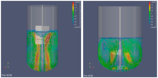
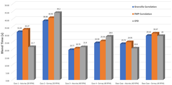
Figure 12.
Mixing hydrodynamics and blend times.
3.2.2. Reactor Yield Mixing-Based Investigation
CFD was used to investigate the impact of mixing on yield during the production of a fine chemical using the first commercial campaign. Here, both empirical and CFD studies were undertaken to compare the agitation profiles within glass-lined and stainless steel reactors at a third-party manufacturing site.
Key differences in the two different mixing vessels were identified, which include:
- Fluid flow and hydrodynamics (i.e., vortex formation);
- Mixing performance (dead velocity zones, flow recirculation regions).
This case study, as illustrated in Figure 13, demonstrated how CFD modeling could be used to

Figure 13.
Reactor yield investigation (glass-lined vs. stainless steel), free surface velocity, and micro-mixing times.
- Evaluate the impact of mode of addition of reactants;
- ○
- Top surface vs subsurface loading provided the opportunity to increase yield, batch size, improve cycle time and increase production rates.
- Investigate new reactor designs for upcoming/new commercial campaigns when there is a question about yield performance for mixing sensitive reactions, impeller location, retrofit tank shape, or optimal batch size.
- Understand key mixing scenarios affecting the yield performance of the cyclization step of the chemical manufacturing process.
Field observations illustrated that yield performance directly correlated to the mixing performance identified through CFD simulations.
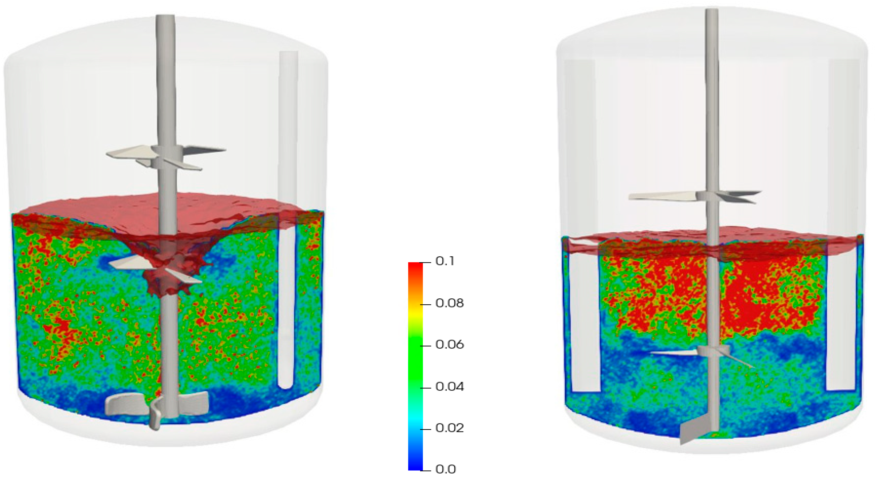
3.2.3. Non-Newtonian Miscible Fluid Mixing in Formulations
This next case-study is for a formulations process at Valdosta, GA, where poor flow at the top liquid surface resulted in extended blend/mixing times. As a result, the batch processing volumes reduced from 9k->7k gal, resulting in extended processing/cycle times. Here, CFD modeling was used for the following:
- Proposing optimal impeller designs (narrow blade hydrofoils) and optimal impeller placement with original batch size.
- Investigating single phase and miscible non-Newtonian fluid blending.
- Quantifying the effect of miscible fluid blending on velocity profiles, blend times and power consumption.
Figure 14 illustrates how CFD helped in the following:

Figure 14.
Non-Newtonian fluid mixing, top free surface velocity, miscible phase volume fraction, and blend time comparison.
- Modeling single phase and miscible non-Newtonian fluid blending.
- Quantifying the effect of non-Newtonian flow on velocity profiles.
- Quantifying the effect of miscible fluid blending on the following:
- ○
- Velocity profiles;
- ○
- Blend times;
- ○
- Power consumption.
- Determining the optimal impeller placement for blend time reduction.
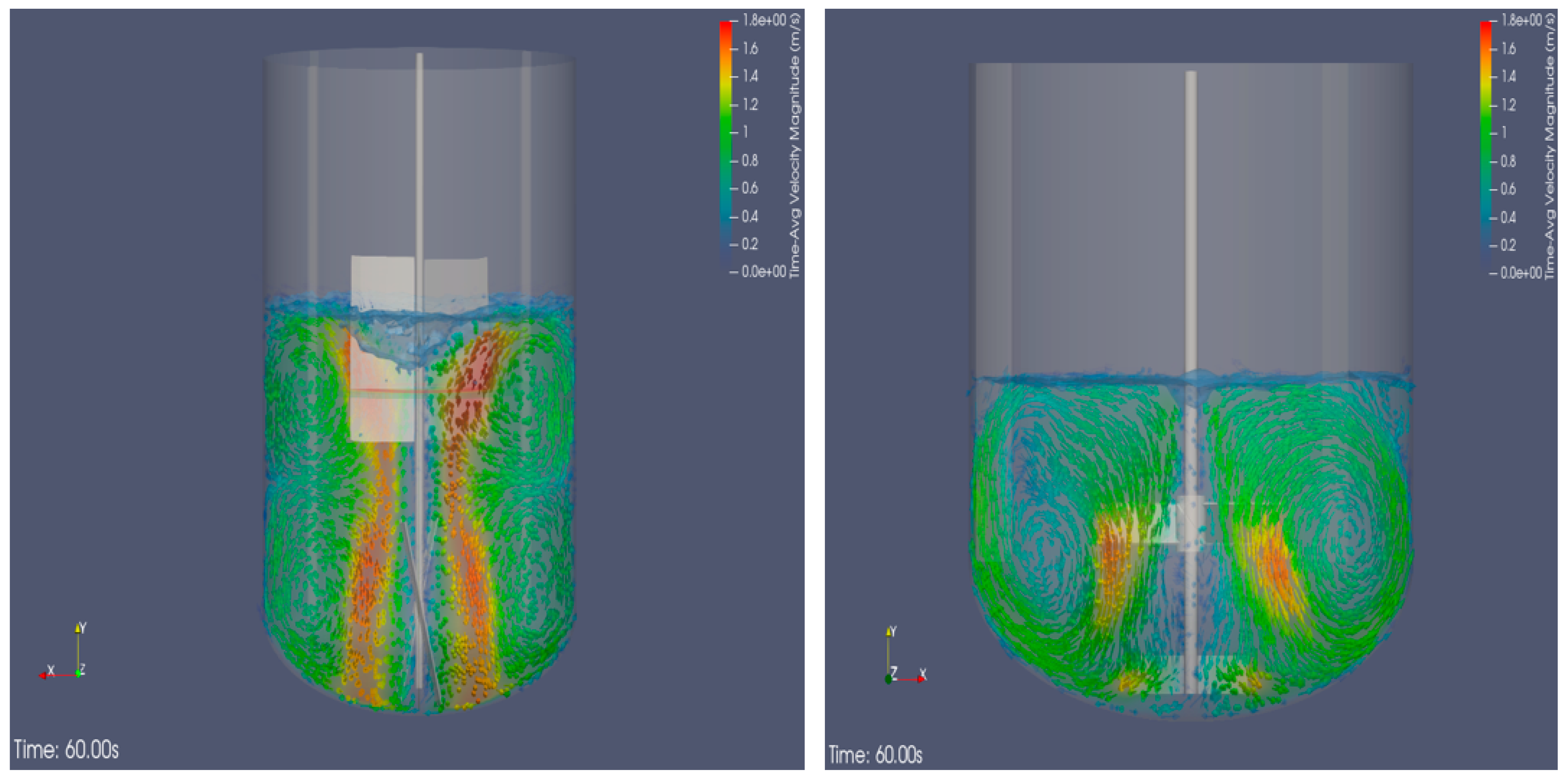
3.2.4. Agitation Design Modifications in Formulations
This example is for a formulation solid–liquid mixing case in a gel tank that did not incorporate xanthan gum powder into water as expected. As a result, powder was floating on the liquid surface and was not being drawn down by the sawtooth blade shear impeller. This led to production delays and forced the gel to be prepared in another area of the plant and transferred via totes. This resulted in added costs for the fleet of totes, adjusting the schedules of other production units, and concerns about the operation of the gel tank. CFD modeling was used here to propose agitation design modifications, enhancing the tank and subsequent formulation processes up to design rates (by as much as 15%).
Figure 15 illustrates how CFD was used in the following:

Figure 15.
Gel tank agitator design modifications, and the effect on flow and blend times.
- Validation of modifications to agitator design with the addition of a second hydrofoil impeller.
- Comparison of current and modified designs.
The base design showed no vortexing during simulations, in comparison to the modified design, which illustrated a strong vortex development 18 s into the simulation. A higher velocity was observed in the entire tank in the modified design, as compared to the base scenario.
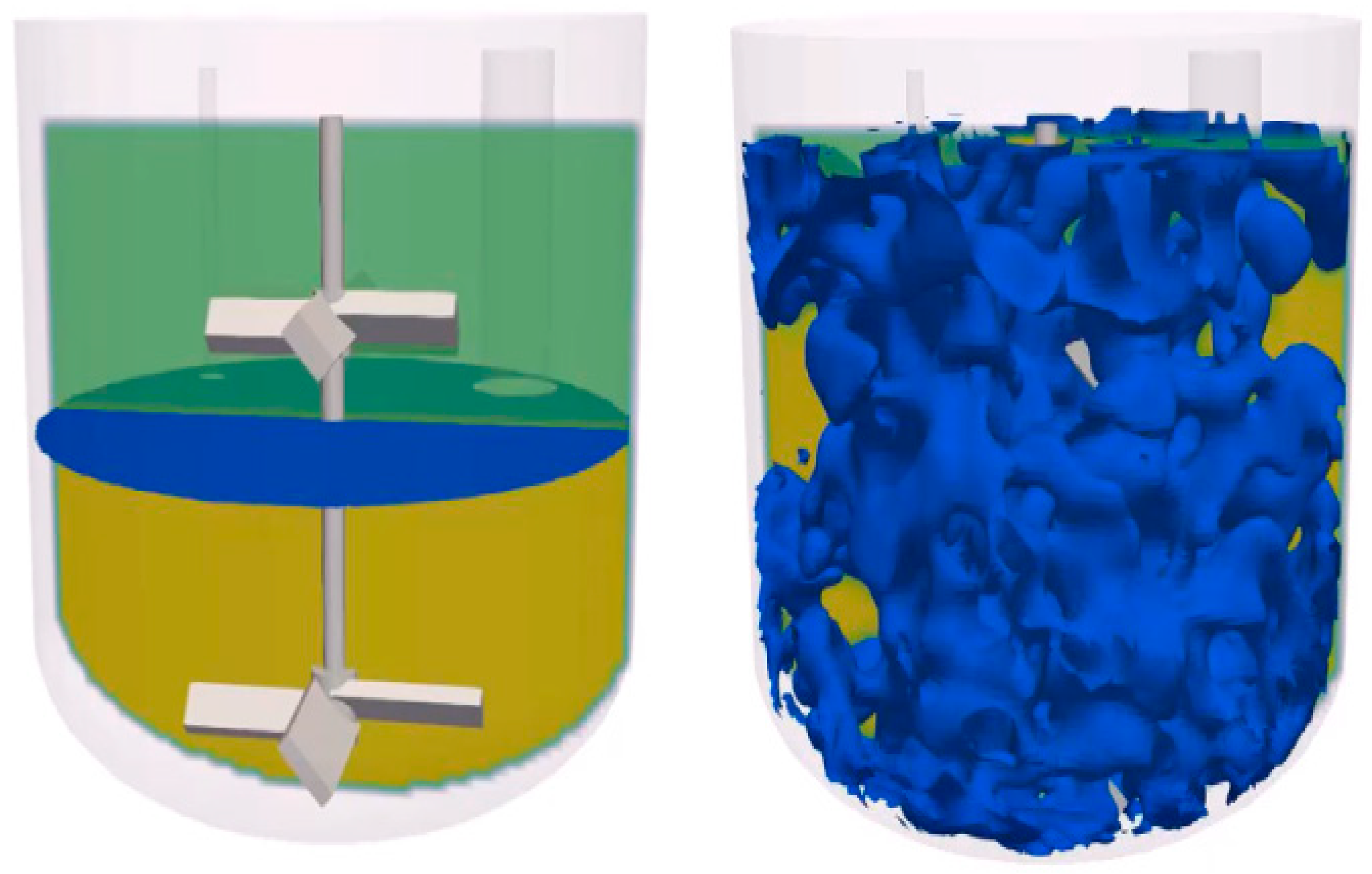
3.2.5. Bi-Phasic Immiscible Mixing CFD Model
This example corresponds to the acidic hydrolysis of an organic toluene bi-phasic system in which two immiscible liquids sit on top of each other. CFD was utilized to predict the range of agitation speeds at which the two liquid layers would break apart and mix with each other, resulting in an increased interfacial surface area. CFD simulations helped to predict the dispersed speed and the contact interfacial surface area between the immiscible phases.
Figure 16 illustrates how CFD was used for this immiscible liquid–liquid mixing scenario. The following were noticed:

Figure 16.
Bi-phasic immiscible mixing model and interfacial liquid–liquid layer at two different operating RPMs.
- Increasing the thermowell ID from 0.125″ to 0.375″ at 100 RPM does not help break up the toluene–HCl layer.
- Introducing baffles with thermowell and pH probes does not help the liquid layer to break up when operating RPM < Njd (just dispersed speed).
- Increasing agitation to 500 RPM breaks up the two liquid layers, inducing maximum interfacial surface area.
CFD can therefore help with predicting dispersed speed and interfacial surface area, and in designing lab scale experiments.
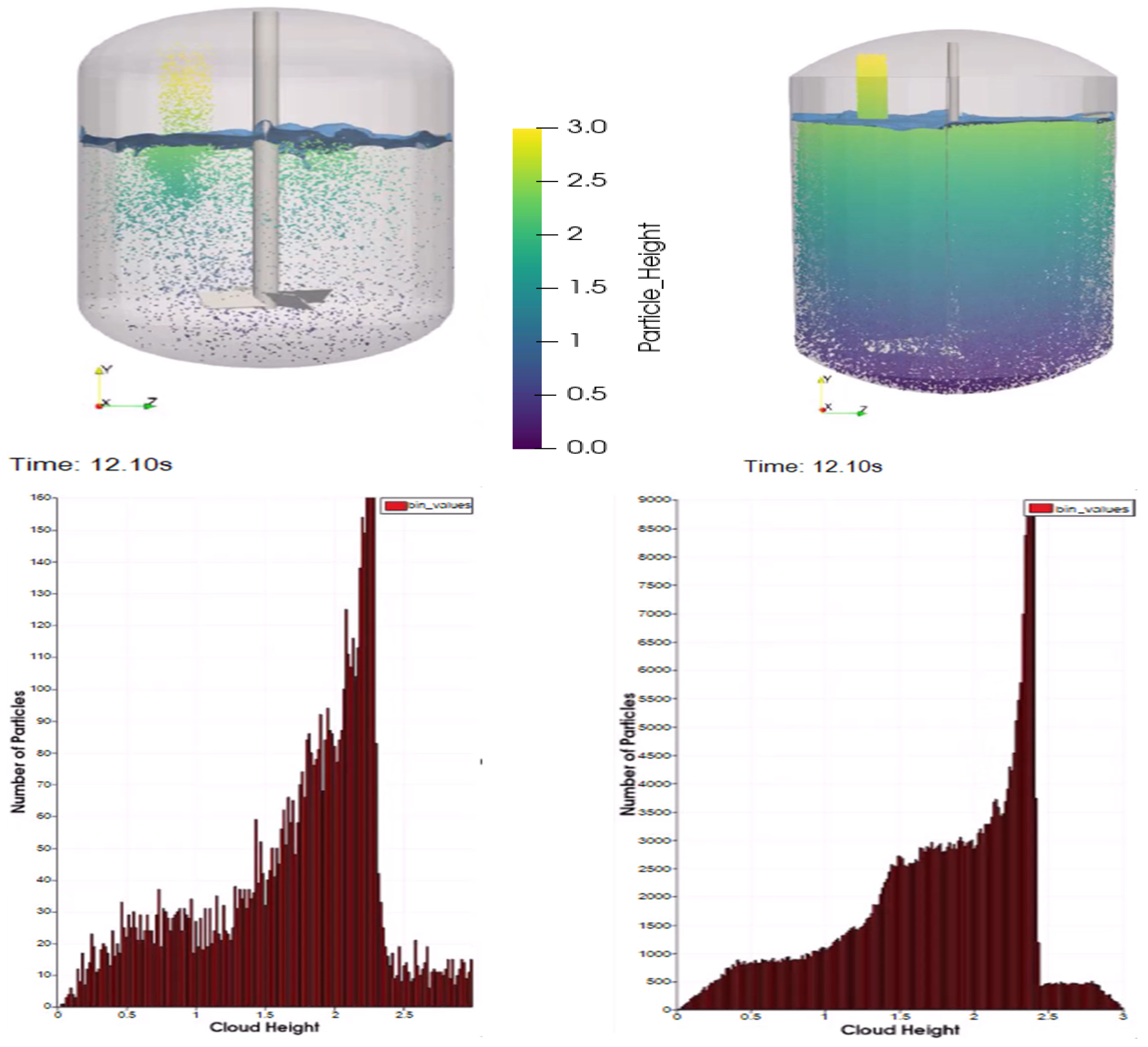
3.2.6. Solid–Liquid Mixing in Formulations
The case study focuses on the solid–liquid mixing formulation process to incorporate floating powder particles within the bulk liquid.
Figure 17 illustrates how CFD was used for the following:

Figure 17.
Solid–liquid mixing for formulations and particles colored by velocity-Y component and cloud height.
- To determine if the operating RPM was sufficient to entrain the powder particles in the bulk liquid.
- To quantify the effect of powder incorporation on velocity, blend times, power consumption, and cloud heights.
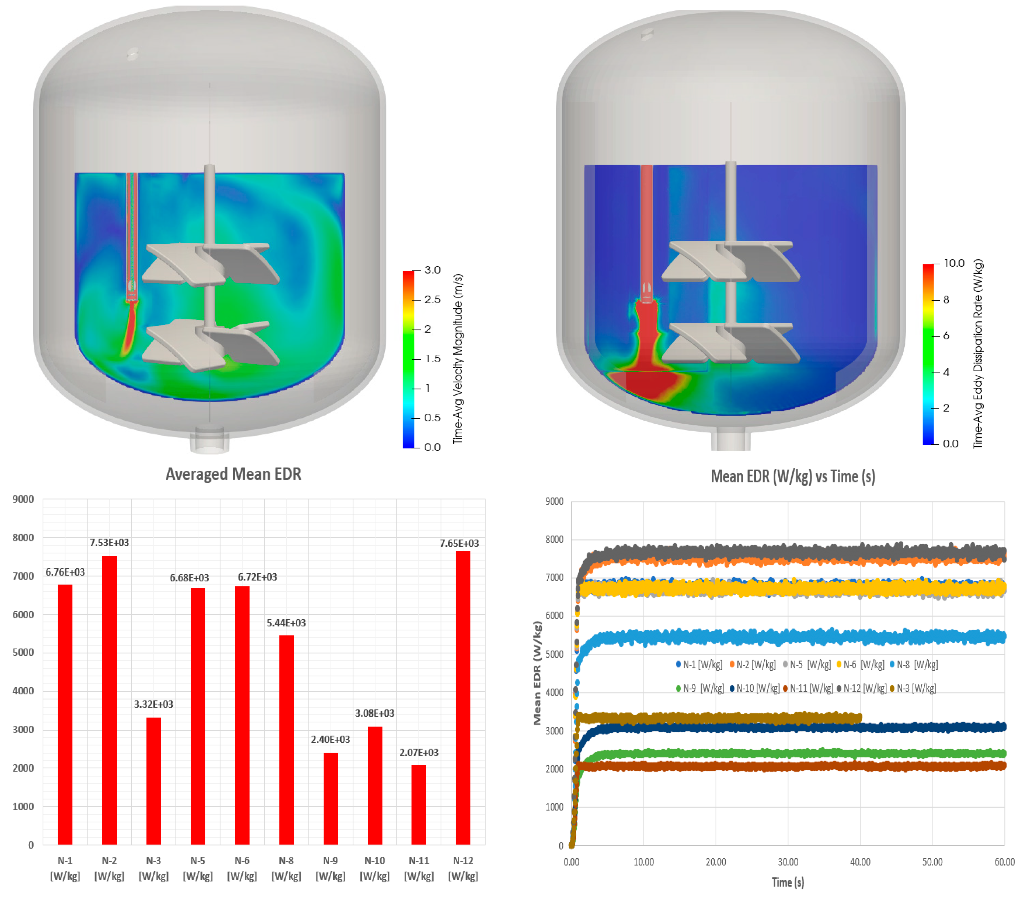
3.2.7. Static Mixer Flow Modeling for Nozzle Design Comparison
Next, we have an example that relates to a drying unit operation which experienced plugging/fouling. CFD was utilized to investigate 12 different static mixer nozzle designs and identify one which promotes the highest droplet break-up. A specific laser-scanned nozzle provides a higher turbulent dissipation rate and a higher pressure drop, indicating a better droplet breakup capability and finer particle size while reducing the possibility of fouling.
CFD, as illustrated in Figure 18, was used for the following:
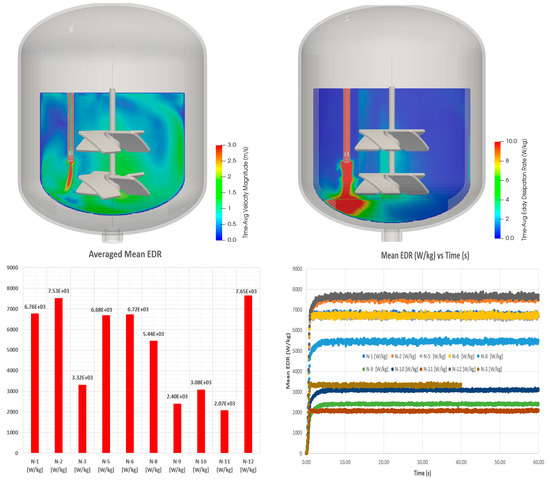
Figure 18.
Static mixer nozzle flow model; base case mixing and nozzle design comparison.
- To understand the impact of key dimensions in the static mixer nozzle design.
- To quantify the impact of nozzle dimensions on the energy dissipation rate and droplet break-up through the simulation of turbulent energy dissipation rates.
- To compare twelve different nozzle variants for reducing fouling.
3.2.8. Jet Mixing Modeling
This example refers to computing blend times for a jet mixing process in non-standard vessel geometries for which empirical correlations are not available. We first built a CFD model to simulate the transient jet mixing hydrodynamics in a vessel with a flat bottom and compared the blend times predicted using CFD to those obtained using empirical correlations. Once we were confident in the CFD predictions, we further extended our CFD modeling approach to compute jet mixing blend times in dished vessels, as illustrated in Figure 19.
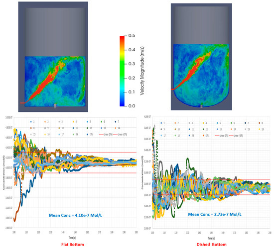
Figure 19.
CFD modeling of jet mixing, velocity profiles, and tracer concentrations for blend time determination.
CFD, as illustrated in Figure 19, was used for the following:
- To model flow hydrodynamics in continuous flow systems like jet mixers with flat and dished bottom heads.
- To quantify the effect of inlet nozzle flow and tank bottom head geometry on the following:
- ○
- Mixing hydrodynamics;
- ○
- Mixing/blend times;
- ○
- Spatial/transient tracer concentration.
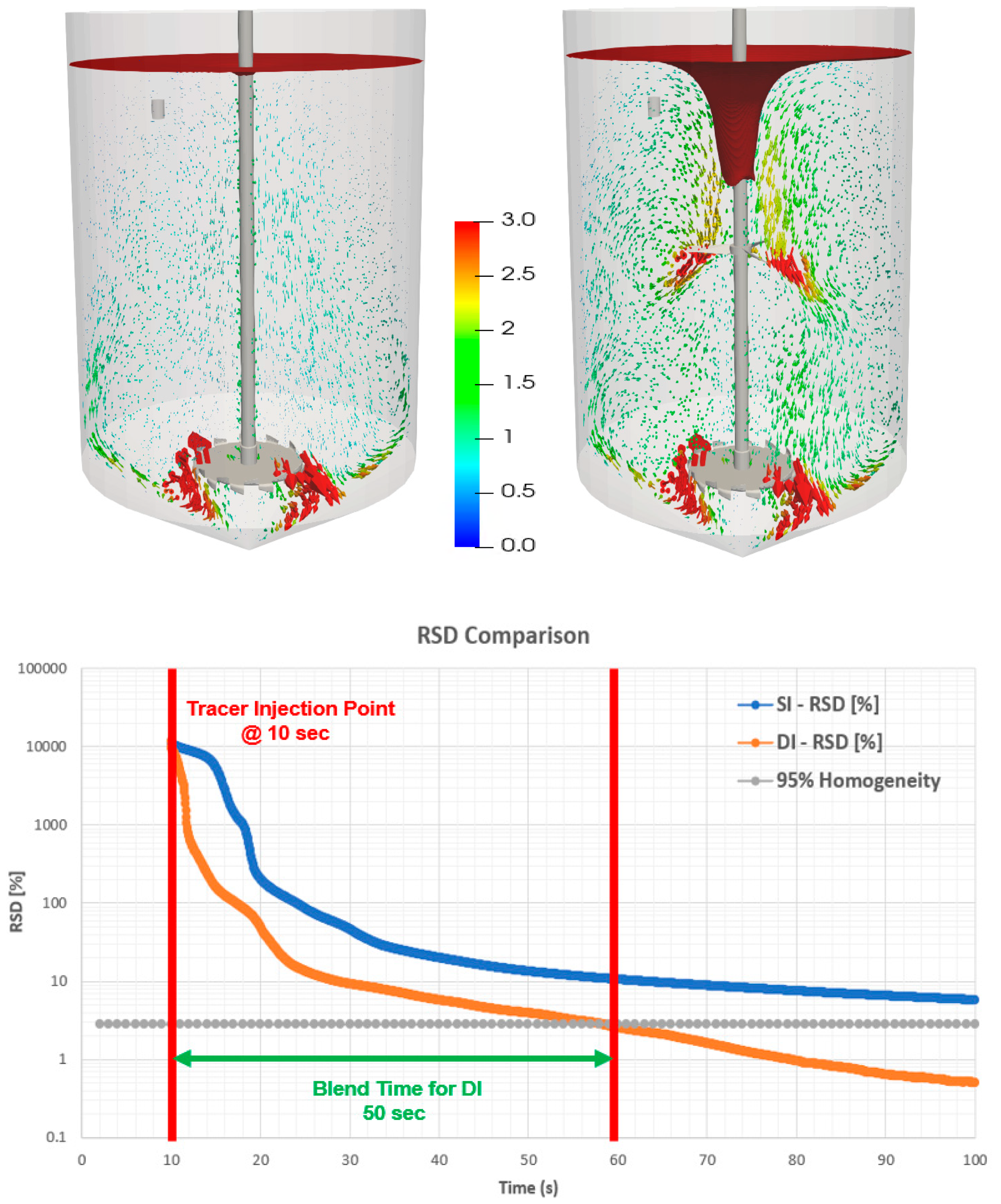
3.2.9. Continuous Flow Process CFD Modeling
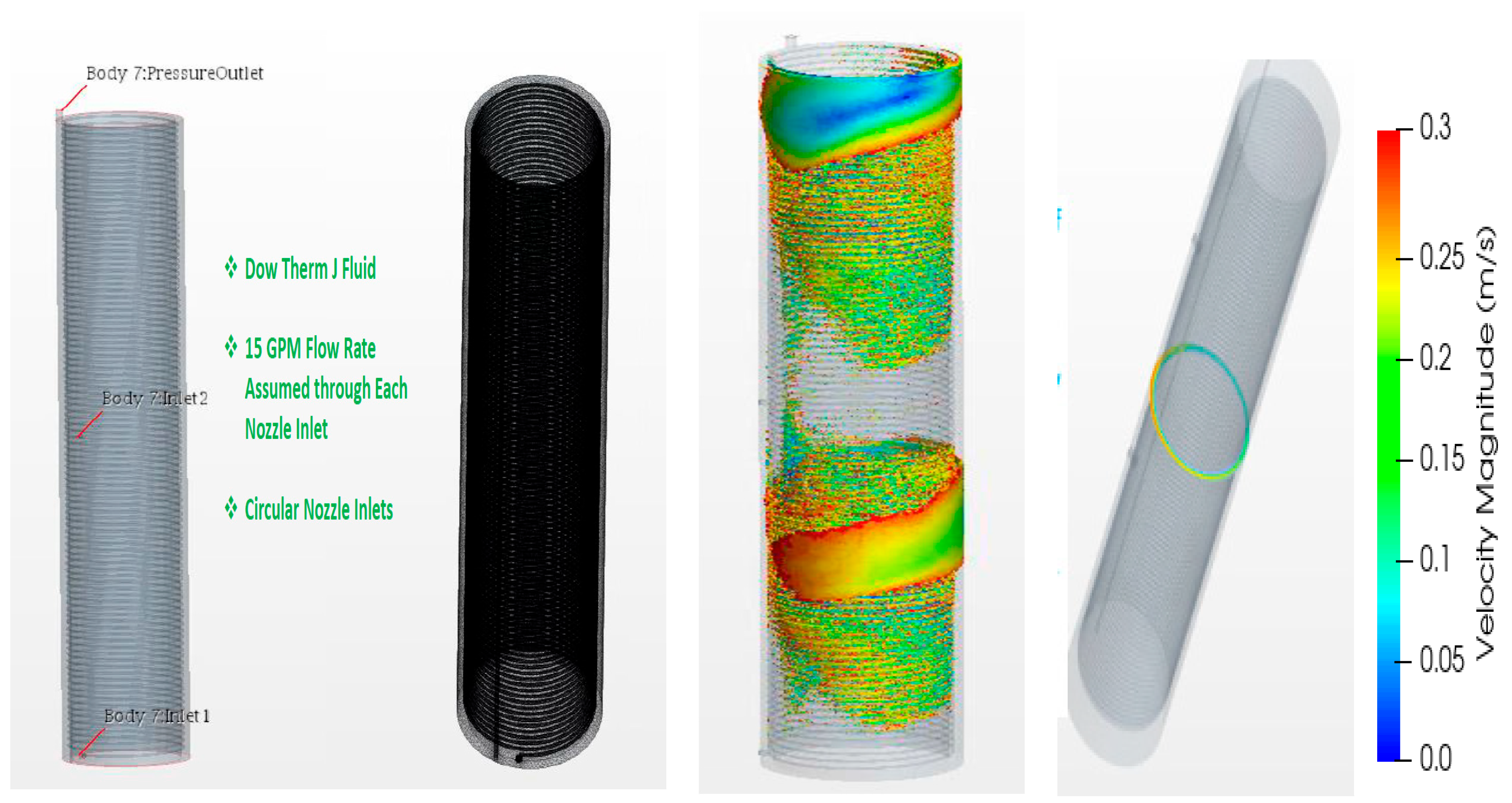
A reaction was being carried out in a coiled reactor. Optimizing the heat exchanger fluid velocity profile through the reactor shell was critical to maintaining the appropriate temperature profile and heat removal rate. As such, agitating nozzles needed to be designed with an optimized nozzle size, no. of nozzles, and vertical position(s) in the shell considering fluid and flow properties, to provide a spiral flow and hence turbulence.
CFD was leveraged to provide insights into the velocity profile as a function of the variables mentioned above. As illustrated in Figure 20, CFD was used for the following:

Figure 20.
Continuous flow processes, velocity profile in volume, and cross-section.
- To quantify the (%) volume of annular flow region within given thresholds.
- To guide the optimal nozzle placement in a continuous flow reactor for minimizing dead zones associated with low velocity thresholds.
- To quantify the effect of viscosity on velocity profiles, and in turn its effect on the wall heat transfer coefficient.
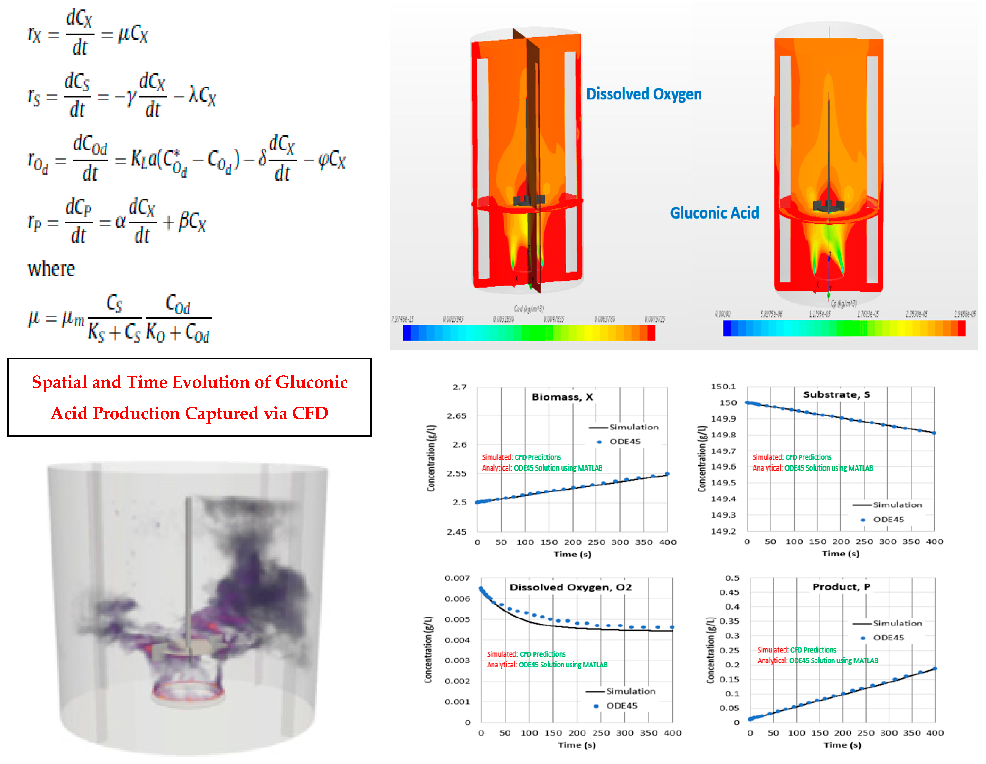
3.2.10. Fermentation, Integrating Biochemical Kinetics with CFD
Finally, we highlight an approach to integrate the unstructured biochemical reaction kinetics with our existing Lattice Boltzmann-based CFD modeling framework (Hanspal et al., 2023 [32], Hanspal et al. [33], Hanspal and Thomas [34], Yeoh et al., 2004, 2005 [35,36], Sirasitthichoke et al., 2022 [37]). This case study involves the application of a Euler–Lagrange CFD approach for the simulation of gluconic acid production based on Contois chemical kinetics published in the literature. Sample results illustrate the time evolution of species concentrations, including glucose, dissolved oxygen, gluconic acid, and biomass, which have been simulated using CFD and compared against the ordinary differential equation (ODE)-based solution implemented in MATLAB (R2020a). Illustrated in Figure 21 are the spatially varying heterogeneous distributions of gluconic acid in the system that can result in an overall yield loss for the fermentation process.
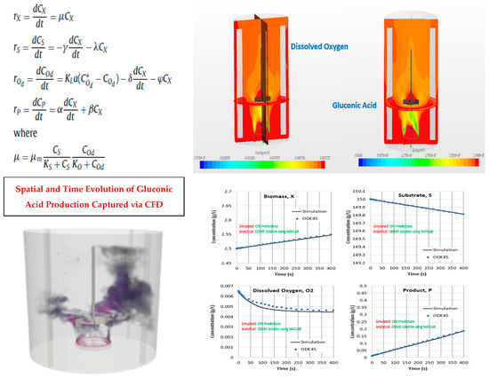
Figure 21.
Fermentation, integrating biochemical kinetics with CFD.
A CFD modeling approach, including the unstructured kinetics (illustrated in Figure 21), was used to simulate the following (Hanspal et al. [33]):
- Heterogeneous distribution of gluconic acid that can result in an overall yield loss.
- Slight differences in DO concentration between CFD and perfectly mixed ODE solution.
- Differences in the results caused by the underlying spatial variations in the gas–liquid mass-transfer coefficient across fluids.
4. Discussion
CFD is the numerical solution to the Navier–Stokes equation (conservation of momentum), continuity equation (conservation of mass), and energy equation (all are partial differential equations—several analytical solutions with various limits, but most applications need to be solved numerically). CFD is used to solve these governing equations and finite volume/element/difference techniques. Many examples in manufacturing and throughout R&D have been provided to highlight the types of problems that can be investigated. Since CFD is based on theory, there are a vast array of other problems that can be explored.
As shown in this work, CFD has been used in a plethora of R&D projects. For example, COMSOL was used to estimate pesticide uptake in humans via inhalation when little or no prior knowledge is available and/or experiments cannot be performed (since humans cannot be tested on experimentally). It was found the pesticide 1,3-D readily adsorbed immediately during inhalation and never reached deep into the lung tissue, which could never have been found out without CFD. These CAT scan files for humans and rats exist and can be used for any volatile material, including volatile pesticide metabolites. These computational approaches using CFD can help avoid the 10x safety factor assigned by regulatory bodies in going from rat to human.
Subsequently, Corteva’s Global Active Process Technology Expertise Center (GAPTEC) group acquired the CFD tool MStarCFD, which is based on the Lattice Boltzmann approach and has been successfully used to study and investigate a variety of continuous flow and batch processes involving mixing as the key unit operation. The key outcomes when applying MStarCFD have been in troubleshooting existing processes, retrofitting existing agitation designs, and proposing new mixing systems/designs that can increase the efficiency, enhance the productivity, and reduce batch cycle or processing times, leading to increased cost savings and revenue.
As illustrated through diverse examples presented in this manuscript, CFD is quite valuable in the following areas:
- For extrapolating field study observations to different and diverse scenarios or when testing on mammals such as humans cannot be performed.
- For achieving a better understanding of the physical phenomena in mixing-based processes.
- For prototyping mixing designs at manufacturing scale cost-effectively, as compared to experiments.
- Understanding transient effects and mixing heterogeneities during scale-up.
Henceforth, CFD has led to many engineering solutions for Corteva problems, as documented by the many publications and examples listed, while increasing our understanding of experimental observations and mixing processes. This paper provides examples in industrial manufacturing and R&D to offer a flavor of the types of simulations that have been historically performed and to offer insights for other projects to pursue.
5. Future Work
Scientists at Corteva have been on the cutting edge of CFD advancement as relevant to the agricultural industry, utilizing various techniques to overcome the numerical problems and to increase speed as problems continue to grow in size. Architecture is now focused on multi-core cloud or grid-computing CPUs and GPUs. In addition, the coupling of machine learning approaches with CFD is coming to the forefront (Vinuesa and Brunton 2022 [38]; Panchigar et al., 2022 [39]), and many commercial software companies offer this coupling in their most recent versions (e.g., SmartUQ, COMSOL, Ansys, Altari, etc.).
Author Contributions
N.H. contributed the manufacturing examples using MstarCFD, STAR-CCM+ and MATLAB, and S.A.C. contributed to the general R&D section using COMSOL Multiphysics and Fluent CFD software. N.H. and S.A.C. were responsible for conceptualization, methodology, use of commercial software packages, validation, formal analysis, and writing this manuscript. All authors have read and agreed to the published version of the manuscript.
Funding
This research received no external funding and was entirely supported by Corteva Agrisciences.
Data Availability Statement
Data are unavailable due to commercial confidential privacy restrictions.
Acknowledgments
All work was supported by Corteva Agriscience.
Conflicts of Interest
Navraj Hanspal and Steven A. Cryer were employed by Corteva at the time of this publication, and this information went through Corteva’s Information Release process before being published. The research was conducted in the absence of any commercial or financial relationships that could be construed as a potential conflict of interest.
Nomenclature
| C | concentration [g·m−3] |
| D | diffusion coefficient [m2·s−1] |
| u = V | velocity vector [m·s−1] |
| p | pressure [kg·m−1·s−2] |
| F = fG | external body forces acting on the fluid (such as gravity) [kg·m·s−2] |
| μ | dynamic viscosity [kg·m−1·s−1] |
| ζ | kinematic viscosity [m2·s−1] |
| ρ | fluid density [kg·m−3] |
| I | identity matrix |
| T | temperature [°K] |
| τ | shear stress tensor [kg·m−1·s−2] |
| D/Dt | material derivative (the rate of change following a moving fluid parcel) [s−1] |
| k | material thermal conductivity [W·m−1·°K−1] |
| et | specific internal energy (internal energy per unit mass) [J·kg−1] |
| Sg | generation source term for energy (radiation effects, thermal heating from electrical current, etc.) [W·m−1] |
| Cv | heat energy absorbed/released per unit mass (constant volume) [J·kg−1·°K−1] |
References
- Yuan, X.; Chai, Z.; Wang, H.; Shi, B. A generalized lattice Boltzmann model for fluid flow system and its application in two-phase flows. Comput. Math. Appl. 2020, 79, 1759–1780. [Google Scholar] [CrossRef]
- Lallemand, P.; Luo, L.S.; Krafczyk, M.; Yong, W.A. The lattice Boltzmann method for nearly incompressible flows. J. Comput. Phys. 2021, 431, 109713. [Google Scholar] [CrossRef]
- Succi, S. The Lattice Boltzmann Equation for Fluid Dynamics and Beyond; Oxford University Press: Oxford, UK, 2001. [Google Scholar]
- Shu, C.; Guo, Z. Lattice Boltzmann Method and Its Application in Engineering; World Scientific: Hackensack, NJ, USA, 2013. [Google Scholar]
- Kruger, T.; Kusumaatmaja, H.; Kuzmin, A.; Shardt, O.; Silva, G.; Viggen, E. The Lattice Boltzmann Method: Principles and Practice; Springer: Cham, Switzerland, 2017. [Google Scholar]
- Sukop, M.; Thorne, D. Lattice Boltzmann Modeling: An Introduction for Geoscientists and Engineers; Springer: Berlin/Heidelberg, Germany, 2006. [Google Scholar]
- Pachpute, S.N. An Introduction to Computational Fluid Dynamics (CFD). Basics of CFD Modeling for Beginners CFD Flow Engineering. Available online: https://cfdflowengineering.com/basics-of-cfd-modeling-for-beginners/ (accessed on 11 August 2024).
- Ray, B.; Bhaskaran, R.; Collin, L. Introduction to CFD Basics; Cornell University: New York, NY, USA, 2012; Available online: https://dragonfly.tam.cornell.edu/teaching/mae5230-cfd-intro-notes.pdf (accessed on 11 August 2024).
- Tu, J.; Yeoh, G.H.; Liu, C.; Tao, Y. Computational Fluid Dynamics: A Practical Approach, 3rd ed.; Butterworth-Heinemann, Elsevier Science: Amsterdam, The Netherlands, 2018; 498p, ISBN 9780081012444. [Google Scholar]
- Tey, W.Y.; Asako, Y.; Sidik, N.A.C.; Goh, R.Z. Governing Equations in Computational Fluid Dynamics: Derivations and A Recent Review. Prog. Energy Environ. 2017, 1, 1–19. [Google Scholar]
- Bournet, P.-E.; Rojano, F. Advances of Computational Fluid Dynamics (CFD) applications in agricultural building modelling: Research, applications and challenges. Comput. Electron. Agric. 2022, 201, 107277. [Google Scholar] [CrossRef]
- Kanti, P.K.; Chandran, S.A. A Review Paper on Basics of CFD and Its Applications. 2016. Available online: https://api.semanticscholar.org/CorpusID:212454797 (accessed on 11 August 2024).
- Hosain, M.L.; Fdhila, R.B. Literature Review of Accelerated CFD Simulation Methods towards Online Application. Energy Procedia 2015, 75, 3307–3314. [Google Scholar] [CrossRef]
- Soodmand, A.M.; Azimi, B.; Nejatbakhsh, S.; Pourpasha, H.; Farshchi, M.E.; Aghadasinia, H.; Mohammadpourfard, M.; Heris, S.Z. A comprehensive review of computational fluid dynamics simulation studies in phase change materials: Applications, materials, and geometries. J. Therm. Anal. Calorim. 2023, 148, 10595–10644. [Google Scholar] [CrossRef]
- Bird, R.B.; Stewart, W.E.; Lightfoot, E.N. Transport Phenomena; John Wiley & Sons: New York, NY, USA, 1960; ISBN 978-0-470-11539-8. [Google Scholar]
- Randles, A.; Kaxiras, E. Parallel in time approximation of the lattice Boltzmann method for laminar flows. J. Comput. Phys. 2014, 270, 566–586. [Google Scholar] [CrossRef]
- Kabilan, S.; Lin, C.L.; Hoffman, E.A. Characteristics of airflow in a CT-based ovine lung: A numerical study. J. Appl. Physiol. 2007, 102, 1369–1482. [Google Scholar] [CrossRef] [PubMed]
- Longest, P.W.; Holbrook, L.T. In silico models of aerosol delivery for the respiratory tract- Development and applications. Adv. Drug Deliv Rev. 2011, 64, 296–311. [Google Scholar] [CrossRef]
- Garcia, G.J.; Schroeter, J.D.; Segal, R.A.; Stanek, J.; Foureman, G.L.; Kimbell, J.S. Dosimetry of nasal uptake of water-soluble and reactive gases: A first study of interhuman variability. Inhal. Toxicol. 2009, 21, 607–618. [Google Scholar] [CrossRef]
- Schroeter, J.D.; Kimbell, J.S.; Gross, E.A.; Willson, G.A.; Dorman, D.C.; Tan, Y.M.; Clewell, H.J., III. Application of physiological computational fluid dynamics models to predict interspecies nasal dosimetry of inhaled acrolein. Inhal. Toxicol. 2008, 20, 227–243. [Google Scholar] [CrossRef]
- Corley, R.; Kabilan, S.; Kuprat, A.P.; Carson, J.P.; Minard, K.R.; Jacob, R.E.; Timchalk, C.; Glenny, R.; Pipavath, S.; Cox, T.C.; et al. Comparative Computational Modeling of Airflows and Vapor Dosimetry in the Respiratory Tracts of Rat, Monkey, and Human. Toxicol. Sci. 2012, 128, 500–516. [Google Scholar] [CrossRef]
- Quinn, A.D.; Wilson, M.; Reynolds, A.M.; Couling, S.B.; Hoxey, R.P. Modeling the dispersion of aerial pollutants from agricultural buildings-an evaluation of computational fluid dynamics (CFD). Comput. Electron. Agric. 2001, 20, 219–235. [Google Scholar] [CrossRef]
- Cryer, S. Predicted Gas Loss of Sulfuryl Fluoride and Methyl Bromide During Structural Fumigation. J. Stored Prod. Res. 2008, 44, 1–10. [Google Scholar] [CrossRef]
- Cryer, S.A.; Barnekow, D.E. Estimating Outside Air Concentrations surrounding Fumigated Grain Mills. Biosyst. Engr. 2006, 94, 557–572. [Google Scholar] [CrossRef]
- Mao, M.; Cryer, S.A.; Altieri, A.; Havens, P. Predicting Pesticide Volatility Through Coupled Above- and Belowground Multiphysics Modeling. Environ. Model. Assess. 2018, 23, 560–582. [Google Scholar] [CrossRef]
- Wolters, A.; Leistra, M.; Linnemann, V.; Klein, M.; Schäffer, A.; Vereecken, H. Pesticide volatilization from plants: Improvement of the PEC model PELMO based on a boundary-layer concept. Environ Sci Technol. 2004, 38, 2885–2893. [Google Scholar] [CrossRef] [PubMed]
- Yates, S.; Wang, D.; Papiernik, S.K.; Gan, J. Predicting pesticide volatilization from soils. Environmetrics 2002, 13, 569–578. [Google Scholar] [CrossRef]
- Altieri, A.L.; Cryer, S.A.; Acharya, L. Mechanisms, Experiment and Theory of Liquid Sheet Breakup and Drop Size from Agricultural Nozzles. At. Sprays 2014, 24, 695–721. [Google Scholar] [CrossRef]
- Cryer, S.A.; Altieri, A.L. Use of large inhomogeneity’s to initiate sprayed sheet demise during atomization. Biosyst. Eng. 2017, 163, 103–115. [Google Scholar] [CrossRef]
- Altieri, A.L.; Cryer, S.A. Break-up of sprayed emulsions from flat-fan nozzles using a hole kinematics model. Biosyst. Eng. 2018, 169, 104–114. [Google Scholar] [CrossRef]
- Krishnan, G.; Cryer, S.A.; Turner, J.; Rajan, N.S. Spray Atomisation in Multiphase Flows with References to Tank Mixes of Agricultural Products. Biosyst. Eng. 2022, 223, 232–248. [Google Scholar] [CrossRef]
- Hanspal, N.; Chai, N.; Allen, B.; Brown, D. Applying multiple approaches to deepen understanding of mixing and mass transfer in large-scale aerobic fermentations. J. Ind. Microbiol. Biotechnol. 2020, 47, 929–946. [Google Scholar] [CrossRef]
- Hanspal, N.; Thomas, J.; DeVincentis, B. Modeling Multiphase Fluid Flow, Mass Transfer, and Chemical Reactions in Bioreactors using Large-Eddy Simulation. Eng. Life Sci. 2023, 23, e2200020. [Google Scholar] [CrossRef] [PubMed]
- Hanspal, N.; Thomas, J. CFD Modeling of Two-Phase Stirred Bioreaction Systems: Applications of Large-Eddy-Simulation (LES) Simulation. In Proceedings of the 2020 American Institute of Chemical Engineers (AIChE) Annual Meeting, San Francisco, CA, USA, 16–20 November 2020; American Institute of Chemical Engineers: New York, NY, USA, 2020. [Google Scholar]
- Yeoh, S.L.; Papadakis, G.; Yianneskis, M. Determination of mixing time and degree of homogeneity in stirred vessels with large eddy simulation. Chem. Eng. Sci. 2005, 60, 2293–2302. [Google Scholar] [CrossRef]
- Yeoh, S.L.; Papadakis, G.; Yianneskis, M. Numerical Simulation of Turbulent Flow Characteristics in a Stirred Vessel Using the LES and RANS Approaches with the Sliding/Deforming Mesh Methodology. Chem. Eng. Res. Des. 2004, 82, 834–848. [Google Scholar] [CrossRef]
- Sirasitthichoke, C.; Teoman, B.; Thomas, J.; Armenante, P.M. Computational prediction of the just-suspended speed, Njs, in stirred vessels using the Lattice Boltzmann method (LBM) coupled with a novel mathematical approach. Chem. Eng. Sci. 2022, 251, 117411. [Google Scholar] [CrossRef]
- Vinuesa, R.; Brunton, S.L. Enhancing computational fluid dynamics with machine learning. Nat. Comput. Sci. 2022, 2, 358–366. [Google Scholar] [CrossRef] [PubMed]
- Panchigar, D.; Kar, K.; Shukla, S.; Mathew, R.M.; Chadha, U.; Selvaraj, S.K. Machine learning-based CFD simulations: A review, models, open threats, and future tactics. Neural Comput. Applic. 2022, 34, 21677–21700. [Google Scholar] [CrossRef]


Disclaimer/Publisher’s Note: The statements, opinions and data contained in all publications are solely those of the individual author(s) and contributor(s) and not of MDPI and/or the editor(s). MDPI and/or the editor(s) disclaim responsibility for any injury to people or property resulting from any ideas, methods, instructions or products referred to in the content. |
© 2024 by the authors. Licensee MDPI, Basel, Switzerland. This article is an open access article distributed under the terms and conditions of the Creative Commons Attribution (CC BY) license (https://creativecommons.org/licenses/by/4.0/).