Abstract
This study numerically analyzes a submerged horizontal plate (SHP) device subjected to both regular and irregular waves. This device can be used either as a breakwater or a wave energy converter (WEC). The WaveMIMO methodology was applied for the numerical generation and wave propagation of the sea state of the Rio Grande coast in southern Brazil. The finite volume method was employed to solve conservation equations for mass, momentum, and volume fraction transport. The volume of fluid model was employed to handle the water-air mixture. The SHP length (Lp) effects were carried out in five cases. Results indicate that relying solely on regular waves in numerical studies is insufficient for accurately determining the real hydrodynamic behavior. The efficiency of the SHP as a breakwater and WEC varied depending on the wave approach. Specifically, the SHP demonstrates its highest breakwater efficiency in reducing wave height at 2.5Lp for regular waves and 3Lp for irregular waves. As a WEC, it achieves its highest axial velocity at 3Lp for regular waves and 2Lp for irregular waves. Since the literature lacks studies on SHP devices under the incidence of realistic irregular waves, this study significantly contributes to the state of the art.
1. Introduction
The climate crisis, which has been announced since the last century, is now a reality. The Paris Agreement in 2015 and the United Nations Sustainable Development Goals (SDGs) highlight the importance of concrete actions to transform production and development processes [1,2]. Fossil fuels are still the largest source of the global energy matrix. However, the quest for decarbonization and the Net Zero goal of the Paris Agreement are of increasing interest in the development of renewable energy sources [3].
Among the SDGs, SDG 7 (affordable and clean energy) and SDG 13 (climate action) are directly related to this study, since a submerged horizontal plate (SHP) can be used as a wave energy converter (WEC). However, the SHP also acts as a breakwater, consequently working on coastal protection and indirectly achieving SDG 11 (sustainable cities and communities) and SDG 12 (responsible consumption and production). Another relevant mobilization is the United Nations Decade of Ocean Science for Sustainable Development (2021–2030), which also has a direct correlation with this study [2,4].
González et al. [3] claimed regarding wave energy that “it is a reliable source since waves could provide a constant energy supply, which is an advantage compared with wind and solar intermittent energy sources; the time variability of energy supply can be much more accurately predicted” [3] (p. 11). Tavakoli et al. [5] pointed out that “research in the field of ocean engineering is in line with general demands such as environmental sustainability, clean, and affordable energy, and absolute safety”. [5] (p. 20). Wahyudie et al. [6] reported an estimated 32 TW of energy available in the ocean. Out of this potential, 2 TW is in the form of sea wave energy. More specifically, on the south-southeast coast of Brazil, the potential energy values are between 6 and 22 kW/m to wave front (as depicted in Figure 1). The measure of energy per meter of wave front is used since the energy power of a wave is proportional to its height and period [7].
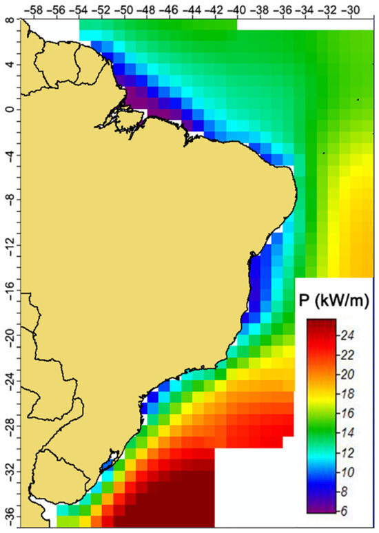
Figure 1.
Average annual power distribution per meter of wave front along the Brazilian coast (adapted from [8]).
The incidence of waves over maritime structures has been widely studied by means of computational fluid dynamics (CFD), which allows investigation of the most different types of applications [9,10,11,12,13,14,15,16,17,18]. Confirming this trend, Opoku et al. [19] explained that research into WEC devices has used CFD as the main source of approach. In this sense, numerical modelling is widely used for the propagation of regular waves in the analysis of WECs, but it is not so frequent to analyze WEC devices when subjected to irregular waves. Studies of irregular waves generally involve the use of wave spectra rather than an actual sea state [20].
Complementary to the objective of reducing carbon emissions through the energy transition to renewable energy sources is the need to protect, adapt, and mitigate the effects caused by extreme events generated by climate change. Tavakoli et al. [5] defined extreme ocean climate events as “strong wind and waves, sea-level rise or loss of ice extents may also necessitate adaptive and mitigative measures.” (p. 2). Muehe [21] estimates that 40% of the Brazilian coast is under severe erosion. This erosion process, as well as damage to constructions in coastal cities, can be intensified as the severity and frequency of climatic events increase. This highlights the relevance of developing coastal erosion protection technologies [22].
In this sense, this work expands scientific investigation through an unprecedented numerical study of the SHP device subjected to representative regular waves and realistic irregular waves of the sea state occurring on the coast of Rio Grande, state of Rio Grande do Sul (RS), in southern Brazil. It is noteworthy that the SHP was originally proposed as a breakwater, but due to its hydrodynamic characteristics, it has been observed in the course of other studies that the SHP can also be used as a WEC. Therefore, the SPH efficiency in both functionalities is numerically evaluated considering five device lengths and keeping constant its submergence depth.
2. Operating Principle, Historical Review, and State of the Art of the SHP Device
The early studies of the SHP as a breakwater in order to attenuate the incident waves date back to the 1950s, by Heins [23] and Greene and Heins [24]; while studies on the WEC function emerged almost 20 years later, starting with Dick and Brebner [25]. After that, other studies were developed, such as Graw [26] and, more recently, Seibt et al. [7].
2.1. Hydrodynamic Principle of the SHP
Analyzing the SHP as a breakwater, the mitigation of coastal erosion is due to the decrease in wave energy and, consequently, the height of the waves after they propagate over the device. In addition, Lima et al. [27] affirm that the SHP has less dependence and influence on local geomorphology and sediment transport conditions than traditional breakwaters because there is no complete reduction in the waves reaching the coast. Still in contrast to a conventional breakwater, the SHP relies not only on fluid-structure interaction but also on fluid-fluid interaction to reflect the waves and reduce the height of the transmitted waves [28,29]; being less dependent on seabed geotechnical conditions where the structure will be installed [30]. Its performance, in terms of cost, is high in relatively deep waters, has no negative effects on the marine landscape, and will never create a zone of standing water, where great efforts are usually needed to maintain water quality [28].
On the other hand, SHP as a WEC is a consequence of experimental analyses. Dick and Brebner [25] were the ones who first observed that due to the propagation of waves over the SHP, the axial velocity of water under the device is sometimes in the direction of wave propagation and sometimes in the opposite direction, generating a pulsating water flow under the structure. Based on that observation, Graw [26] carried out an experimental study on the variation of water flow velocity below the SHP, suggesting that its use as a WEC is possible by inserting a hydraulic turbine below the device.
Figure 2 illustrates a longitudinal section of the SHP structure, making it possible to identify its function as breakwater (due to the reductions of the wave height after the SHP) and its function as WEC (due to the alternating flow under the SHP that can drive a hydraulic turbine).
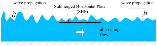
Figure 2.
Submerged horizontal plate device.
2.2. Studies of the SHP as Breakwater
The main goal of the Dick and Brebner [25] study was to develop an empirical and theoretical relationship for the reflection coefficient (Cr) and the transmission coefficient (Ct) through tests with regular sinusoidal waves equivalent to the same wave energy as the irregular wave actually transmitted. The results obtained indicate that the permeable submerged breakwater, for submergence depths greater than 5% of the total depth, transmits less energy than a solid breakwater under a certain frequency range.
Other works have also investigated the Cr and Ct through different waves and computational models. Siew and Hurley [31] investigated the effect of a long wave train on an SHP to design floating breakwaters that are less permanent. Wang and Shen [32] considered the potential analysis of linear waves for a group of SHPs. They obtained the coefficients to evaluate the performance of multiple plates as a breakwater and the effects caused by the gap between the plates. Karmakar and Soares [30] studied the interaction of waves with two floating submerged plates, one of them tilting. The 2D problem was formulated based on linear wave theory. The analysis showed that wave elevation in the transmitted region was lower compared to the incident wave region. Cheng et al. [33] investigated the non-linear transformation and dispersion of incident waves on an SHP in the presence of a uniform stream. It is found that the maximum reflection or minimum transmission for different currents occur at the same plate width because of the compensating Doppler effects of current. The current has a stronger influence on the wave forces than on wave surface elevation. Fang et al. [34] used an analytical model based on potential flow theory. The authors reported a general solution for the hydrodynamic pressure and wave forces exerted on submerged plates. The authors found that the reflection coefficient is sensitive to the peak frequency of the focused wave group and the length of the plate. In addition, the length of the plate significantly alters the hydrodynamic performance, while the height of the plate has little influence.
Yu [28] presented the hydrodynamic effects in relation to the geometry and characteristics of the SHP: plate length, minimum transmission and maximum reflection, installation depth, and others.
Aghili et al. [35] studied the interaction of solitary waves with a SHP. The numerical results indicated that, as the distance of the horizontal plate from the free surface decreases, the energy of the waves propagating past the plate is significantly reduced. However, as the distance of the SHP from the seabed increases, the vertical component of the wave force and its pressure component decrease substantially.
2.3. Studies of the SHP as WEC
Based on the study of Graw [26], Orer and Ozdamar [36] carried out an experimental test in a laboratory wave channel, monitoring the axial velocity under the SHP device for the 2nd order Stokes waves incidence. Results highlighted the existence of horizontal water flow, in both directions, below the SHP. In the pulsating flow, the authors found that the magnitude of the velocity in the opposite direction was greater than the wave propagation.
After that, some investigations have been performed for different aspects of the SHP as a WEC. Wagner et al. [37] explored the hydrodynamics of a submerged WEC using the Green-Naghdi equations with experimental and numerical data. The device’s geometry involves a SHP that oscillates vertically in a range of space. Xu et al. [38] studied the fluid-structure interaction between the solitary wave and the SHP with their own CFD code, MLParticle-SJTU. The results indicate that the effect of the plate on the wave velocity differs under different wave heights.
In its turn, Seibt et al. [39] numerically investigate the effect of the distance from the SHP to the bottom of the channel (hp) on its performance as a WEC using 2nd order Stokes waves. The pulsating flow behavior is in line with previous findings in the literature [36,40]. As a result, the greatest efficiency of SHP occurred in the case of hp = 0.53 m (88% of depth) with a value of 64.0%. Seibt et al. [41] also studied the influence of the opening rate below the SHP on the efficiency of the device as a WEC. Results showed that a 5% increase in aperture rate can increase efficiency by approximately 93%. Besides that, Seibt et al. [42] carried out a numerical study to evaluate the theoretical efficiency for various relative plate heights using 2nd order Stokes waves. Overall, the highest wave power had a 250% increase in maximum axial velocity compared to the lowest. Finally, Seibt et al. [7] applied the Constructal Design in the SHP as WEC. This method allows evaluation of the influence of the geometric configuration on a flow system performance. The authors presented an optimal full-scale geometry defined from the incidence of regular waves corresponding to the 2nd order Stokes wave theory. The degree of freedom optimized in the study was the plate installation height (hp).
2.4. Studies of the SHP as Breakwater and WEC
He et al. [43] developed a two-dimensional numerical study with regular waves and using the numerical method Weakly Compressible Smoothed Particle Hydrodynamics (WCSPH). The authors remark that although SHP attenuates waves and, in the meantime, aids energy acquisition, little effort has been made to combine these two functionalities. Hayatdavoodi et al. [29] presented a numerical study of solitary and cnoidal wave transformation over a SHP using the non-linear Green-Naghdi (GN) Level I equations for shallow waters. The aim of the study was to quantify the dispersion of nonlinear waves as they propagate over the SHP. The conclusions highlight the possibility of SHP as a breakwater and, in shallow waters, as a WEC device. They also mentioned that the ratio of wavelength to plate length and the depth of submergence of the plate play a significant role in SHP’s function as a WEC.
Zheng et al. [44] show an experimental solution to the effect of wave dissipation and the velocity field characteristics at the base of both solid and permeable SHP employing irregular waves. The authors concluded that the attenuation of the wave period (SHP as a breakwater) is more significant when the submerged depth is small; and an adequate rate of transverse openings (holes) in the plate can improve period attenuation. Additionally, the maximum flow velocity of the unperforated plate decreases with increasing relative plate lengths and significant wave heights; and relative depth of the unperforated SHP has no significant effect on the flow velocity. For the range of experiments carried out, the correlation between the transmission coefficient of the solid plate and the maximum velocity at the bottom of the plate is not equally strong compared to the one for the perforated plate.
3. Materials and Methods
Regular wave theories are idealized analytical solutions that are very useful for representing waves in deep water and for structure design. Countless numerical studies have analyzed the performance of WEC with regular waves, even though the ocean surface is irregular [45].
To properly describe the ocean surface, a large number of monochromatic waves with different frequencies and heights must be overlapped. A wave spectrum involves a known amount of energy and is formed by the superposition of nonlinear waves [46]. Spectral analysis increases the accuracy of determining the energy available in ocean waves compared to the monochromatic regular wave models available. The waves for this process are described by the value of the significant height (Hs) of the series, representing the average height of the upper third of the wave height series (H) [47].
This paper analyzes the SHP device for both regular and irregular waves. Both wave series are generated using the WaveMIMO methodology proposed in Machado et al. [20]. The equations of the linear wave theory are used to obtain the orbital velocities over time [48]. What sets this methodology apart from other numerical solutions is its ability to reproduce realistic irregular waves of sea states based on data measured on site or obtained from software such as TOMAWAC (https://www.opentelemac.org/index.php/download) [20].
Linear wave theory is the simplest description of a wave; the trough and crest of the wave are considered to have the same amplitude and the height is considered to be very small compared to the wave’s length (λ). The horizontal component of the wave’s velocity (u) and the vertical component (w), which define the progressive linear wave, are given, respectively, by [46]:
where is the wave frequency (s−1) and is the wave number (m−1).
The 2nd order Stokes wave theory is used in the verifications and validation procedures in this work. The nonlinear theory is applicable on deep water and its perturbation series added to the linear equations improves the analytical description on the relation between the flow velocity and the wave height. The wave profiles are combined to provide a steeper crest and shallower trough and are located at more than half the wave height above the mean water level. This approach delivers more accurate free surface elevation and wave kinematics, which are often considered in the design of coastal and offshore structures [45,46,49]. Its horizontal (u) and vertical (w) components of the wave’s velocity and the water free surface elevation (η) are given, respectively, by [46]:
3.1. Computational Model
Numerical simulations were carried out using ANSYS Fluent software (https://www.esss.com/en/ansys-simulation-software/ansys-fluent-cfd/), which is a CFD package based on the finite volume method (FVM) [50,51,52]. In this study, simplifying hypotheses are applied for the numerical solution of the flow: isothermal, laminar, incompressible, two-dimensional, and transient flow. Thus, the equations of conservation of mass and momentum are defined, respectively, as [53]:
where p is the pressure (Pa), is the density (kg/m3), t is the time (s), is the absolute viscosity coefficient (kg/m·s), is the strain rate tensor (N/m2), and is the damping sink term (N/m3).
To numerically reproduce the interaction between water and air, the volume of fluid (VOF) model proposed by Hirt and Nichols [54] was adopted. This is based upon the premise that the volume of a fluid (q0) cannot occupy the volume of another fluid, which is represented in each control volume of the numerical domain by the volume fraction (αq). The volume fraction transport equation is then added to the model [55] as follows:
where is the velocity vector (m/s).
Once the equations for the conservation of mass and momentum have been solved for the mixture between air and water, the absolute values for density () and viscosity () of the volume fraction are calculated as follows [55]:
According to Srinivasan et al. [56], by treating the phase boundary as an embedded interface and adding the appropriate source terms to the conservation laws, this model consequently allows the identification of the elevation of the free surface. The model considered that when the cell contained only water, when it contained only air, and values of indicated the free surface interface within the cell.
Figure 3 shows the two-dimensional numerical channel geometry with the SHP and the boundary conditions (BC) applied to the model. The dimensions outlined in Figure 3 are wave channel height (Hc); wave channel length (Lc); channel depth (d); horizontal distance from the channel entry to the beginning of the SHP (Xp); SHP length (Lp); SHP depth (hp); SHP thickness (tp); and numerical beach length (Lnb). The dimensions for the verification, validation, and case study processes are presented separately throughout the respective sections.
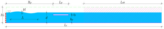
Figure 3.
Numerical wave channel geometry with SHP.
Regarding the BC, the bottom of the channel and the SHP contour, in blue color, are attributed to the condition of impermeable, non-sliding walls, i.e., no mass transport through them. The green dashed line is the pressure outlet. There is a pressure outlet to the right of the channel, the black dotted line, with a constant water depth, known as the hydrostatic profile and allowing the employment of the numerical beach (explained below).
The numerical wave generator located on the left vertical edge of the channel is based on the imposition of the wave’s velocity components, i.e., a BC of prescribed velocity (also called velocity inlet). To generate regular waves, the conventional methodology consists of imposing the velocity components in a continuous line (which would be the line formed by the red and white segments in Figure 3) from the regular theory equations, given by, for instance, Equations (1) and (2) or Equations (3) and (4) [7,49,55]. However, due to the WaveMIMO methodology, the procedure for input velocity BC is imposing prescribed velocity profiles with discrete component data of the u and w velocity components over time in each of the red and white subdivisions of the wave channel entrance region of Figure 3.
Further explanations will be given in Section 3.3. This different way of applying the velocity components is used in all the numerical simulations carried out in this study, since the WaveMIMO allows not only the generation of regular waves but also mainly the generation of irregular waves.
The numerical beach, pink hatched region (see Figure 3), avoids interference with the results due to reflected waves at the end of the channel. Wave damping is in a limited region (Lnb) and ruled by [57]:
where C1 (s−1) and C2 (m−1) are the linear and quadratic damping coefficients, V is the velocity (m/s), z is the vertical position (m), zη and zb are the vertical positions of the free surface and the bottom, respectively, x is the horizontal position (m), and xs and xe are the horizontal positions of the start and end of the numerical beach, respectively. Values of C1 = 20 s−1 and C2 = 0 m−1 were adopted as recommended by Lisboa et al. [57].
The spatial discretization employed the stretched mesh methodology previously used in Gomes et al. [55] and based on Mavriplis [58], where the mesh resolution is increased only in the regions of greatest variation or interest in the result in order to reduce the computational effort. This mesh generation strategy is widely used in numerical simulations of wave generation and propagation and consequently broadly adopted in computational modeling applied to WECs. For the present study, the stretched mesh is employed in the regions before and after the region in which the SHP is located; while in the region of the SHP a quite refined mesh was used in order to capture the fluid dynamic behavior around the device.
The VOF model was chosen with an explicit formulation, and the flows in the cells were interpolated with the Geo-reconstruct scheme. With the Pressure Staggering Option scheme (PRESTO), the pressure on the edges of each cell is interpolated. The Pressure Implicit with Splitting of Operators method (PISO) was used for pressure-velocity coupling [7].
The accuracy of the computational model in relation to the reference data was assessed by a statistical approach. To do this, the mean absolute error (MAE) and root mean square error (RMSE) indicators were used [59], as well as the relative percentage error (RPE) [60] in the verification and validation of the computational model, defined respectively by:
where is the result obtained in this study, is the reference value for comparison, and n is the sample size of the considered data.
Lastly, in order to determine the Hs from the numerical results obtained for the analyses made with representative regular and realistic irregular waves, the OCEANLYZ software (https://github.com/akarimp/Oceanlyz) was used. This software is a toolbox for analyzing wave time series data collected by sensors in open bodies of water, such as oceans, seas, and lakes, or in a laboratory. The software has a graphical interface that allows spectral and wave analysis using the zero-crossing method [61].
3.2. Representative Regular and Realistic Irregular Waves of a Sea State
The WaveMIMO methodology, presented by Machado et al. [20], allows the propagation of a realistic sea state in ANSYS Fluent software by processing the wave spectrum of a desired region. In this work, the wave spectrum is the result of a numerical simulation carried out in the TOMAWAC software for a defined geographical point and time period. Figure 4 is a schematic representation of the data processing stages in this methodology.
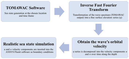
Figure 4.
Schematic representation of the data processing stages in WaveMIMO methodology (adapted from [20]).
In the present study, as in Maciel et al. [62], the application of the WaveMIMO methodology considers the sea state for the region of the municipality of Rio Grande, in the state of Rio Grande do Sul, Brazil. The realistic sea state generated in TOMAWAC is for the period between 1 January and 31 December 2024. The point at which the data for this study were extracted is located at the coordinates 52°17′47.25″ W, 32°22′30.95″ S at a distance of 2 km from the coast and a depth of 9.52 m. This point is called “Node 1545”, as shown in Figure 5.
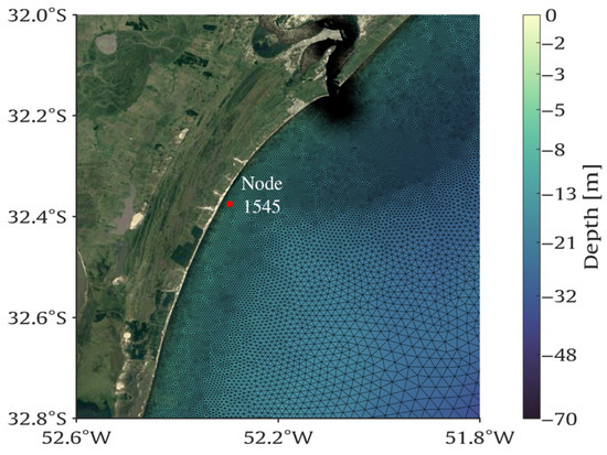
Figure 5.
Location of the realistic sea state extraction point (adapted from [62]).
Once the wave spectrum has been transformed into a time series of free surface elevation, this series is statistically analyzed using a histogram of pairs of significant heights (Hs) and mean wave periods (Tm). For the considered sea state, the wave histogram is shown in Figure 6a, with the most frequent value being the wave with Hs = 0.66 m and Tm = 6.30 s. Figure 6b presents the frequency spectrum with most similar characteristics of the most frequent values from the yearlong series presented in Figure 6a. This spectrum from Figure 6b is actually the one from which the η series is decomposed into the velocity components u and w. These wave characteristics are defined as the representative regular waves of the sea state of Rio Grande. This definition will be an important parameter for the mesh design and to verify the WaveMIMO methodology.
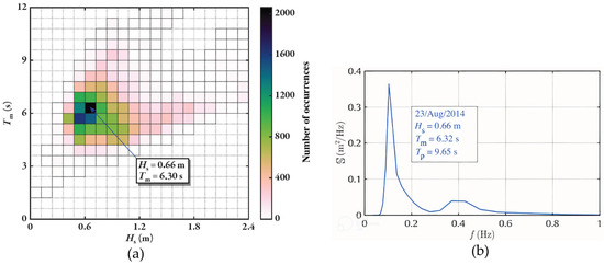
Figure 6.
(a) Histogram with significant wave height and mean wave period of the sea state (adapted from [62]); (b) Variance spectral density as a function of the frequency f of the sea state on 23 August 2014 at 00:00 (adapted from [62]).
In Figure 7, the surface elevation series, i.e., the realistic sea state to be propagated in the numerical simulations of the two-dimensional channel, is shown.
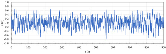
Figure 7.
Free surface elevation (η) of the realistic sea state considered.
The WaveMIMO methodology is applied to the case study, and the geometry of the numerical channel follows the recommendations of Maciel et al. [62]. The wave channel length is 5 times the length of the representative regular waves of the sea state (λ = 51.6 m), obtained from the Hs and Tm. Therefore, the length of the numerical channel is 258 m, the height is 12 m, and the depth is 9.52 m.
To apply the η series in the numerical channel simulation in ANSYS Fluent software requires a transformation of the elevation data into velocity components u and w over time to be imposed as velocity inlet boundary condition. Further information about this data transformation from η to u and w can be found in Machado et al. [20] and Oleinik et al. [48], while Maciel et al. [63] investigated the number of subdivisions of the input velocity imposition region with the aim of achieving maximum approximation between the waves generated in the numerical model and the waves in the elevation series from which the velocities were extracted. The result obtained by Maciel et al. [62] indicates that the velocity inlet region (see Figure 3) must be subdivided into 10 segments. For each of those, the components u and w are determined over time with a fixed depth at the base of the segment. Thus, each of the 10 segments will have its own velocity profiles over time, which allows the generation of representative regular waves and realistic irregular waves of the Rio Grande sea state.
3.3. Verification and Validation Procedures
Initially, the WaveMIMO methodology for generating representative regular and realistic irregular waves of a sea state is verified. Then, considering the presence of SHP in the wave channel, a validation and verification of the computational model adopting the WaveMIMO methodology for generating regular waves are developed. Finally, a verification of the OCEANLYZ software is also performed.
3.3.1. Verification of the WaveMIMO Methodology
The verification of the WaveMIMO methodology is carried out considering the sea state of the coast of the city of Rio Grande, RS, Brazil, for two situations: numerical simulation with representative regular waves (see Figure 6) and numerical simulation with realistic irregular waves (see Figure 7). The simulation lasts 300 s for both cases.
The numerical generation of representative regular waves is verified by comparing the numerical results of this computational model with the analytical solution of the 2nd order Stokes wave theory, as described in Equation (5), from the position of the free surface at coordinate x = 50 m. Meanwhile, the numerical verification of realistic irregular waves is carried out by comparing the numerical results of this computational model at the position of the wave generator (x = 0 m) and the data from the free surface elevation series derived from the TOMAWAC wave spectrum; in other words, with the η series that generated the orbital velocities imposed as BC in the ANSYS Fluent software.
3.3.2. Validation of the Computational Model in a Laboratory Scale with SHP
The computational model was validated with the experimental study of Orer and Ozdamar [36]. The authors analyzed the efficiency of SHP as a WEC. This study was carried out in a laboratory wave channel with a piston-type unidirectional wave generator. The characteristics of the regular waves generated experimentally and reproduced numerically in this work are shown in Table 1, where d/λ is the relative depth.

Table 1.
Characteristics of regular waves for validation.
The numerical model consists of a two-dimensional wave channel with the SHP. For the validation process of the computational model, according to data from Orer and Ozdamar [36], the dimensions of the numerical channel are (see Figure 3) as follows: Hc = 1 m; Lc = 40 m; d = 0.6 m; Lp = 1 m; tp = 0.02 m; and Xp = 19.5 m. The WaveMIMO methodology was used, so the velocity inlet boundary condition was divided into 10 segments and the velocity profiles were inserted for each of them considering the 2nd order Stokes wave theory.
The stretched mesh methodology was used, with spatial discretization in the regions upstream and downstream of the SHP as recommended by Gomes et al. [55]. The water-only region is divided into 60 computational cells; the water-air interaction region has 40 computational cells; and the air-only region has 20 computational cells. Along the channel, the mesh has a discretization of λ/50. Figure 8 shows the mesh around the SHP, with 100 horizontal divisions and the same vertical discretization as before. This change is essential for analyzing the hydrodynamics of the SHP due to the high velocity gradient. Figure 8 depicts in detail the mesh generated in the SHP region, however, it is also possible to observe the stretched mesh generated before and after the SHP.
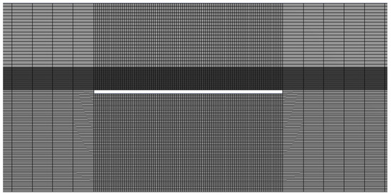
Figure 8.
Computational domain discretization for validation, detailing the regions near the SHP.
For validation, the parameter used is the axial velocity of the water flow at the midpoint between the bottom of the channel and the SHP. The case corresponding to the SHP without any restrictions between it and the bottom of the wave channel was considered. For this case, the installation height of the plate is 0.52 m. The numerical probe is a point (x = 20 m, z = 0.26 m), see Figure 9, to monitor the axial velocity below the SHP and then compare it with the values provided by Orer and Ozdamar [36].
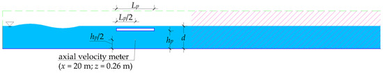
Figure 9.
Numerical probe position for validation.
In the ANSYS Fluent software, the simulation was carried out with a time step of 0.001 s, as in Seibt et al. [7], and a time interval of 25 s was simulated, resulting in 25,000 iterations.
3.3.3. Verification of the Full-Scale Computational Model with SHP
This verification was based on the comparison between the numerical results of Seibt et al. [7] and the numerical results obtained in the present study. While Seibt et al. [7] employed the conventional methodology to the generation of regular waves, i.e., employing Equations (3) and (4); the current study applied the WaveMIMO methodology to do so. Seibt et al. [7] indicated the optimum full-scale dimension of SHP as WEC for the characteristics of regular waves, shown in Table 2. The numerical channel parameters were built with the following dimensions (see Figure 3): Lp = 4.653 m; Xp = 2λ = 139.584 m; Lnb = 2λ = 139.58 m; Lc = Xp + Lp + 1 m + Lnb = 284.82 m; Hc = 16 m; hp = 8.64 m; and tp = 0.32 m.
Table 2.
Characteristics of regular waves for verification.
Another difference between Seibt et al. [7] and the present work concern the spatial discretization. Seibt et al. [7] used a non-homogenous mesh where the horizontal discretization was defined as a function of the third harmonic equivalent wave length (λ3) and the vertical discretization was defined as a function of the wave height (ε), as can be seen in Figure 10. Further details about this spatial discretization can be found in Seibt et al. [7].
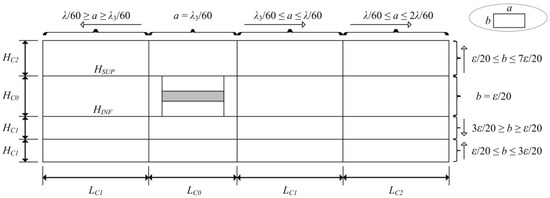
Figure 10.
Mesh used for verification (adapted from Seibt et al. [7]).
In turn, the present work adopts the stretched mesh methodology, with spatial discretization in the regions upstream and downstream of the SHP as recommended by Gomes et al. [55] and already described in the validation methodology. Close to the SHP, 1 m upstream and 1 m downstream are regions of high interest, therefore the horizontal discretization has a 0.05 m dimension, while the vertical discretization respect those of the stretched mesh.
Additionally, another difference is related to the length and right end of the wave channel. In Seibt et al. [7], a longer wave channel having a wall as right end was adopted; while in the present study, a shorter wave channel with a numerical beach after the SHP and a hydrostatic profile as right end was employed by means of Equation (11).
To verify the computational model, the elevation of the free surface before the SHP and the axial velocity of the flow below the SHP were measured. More precisely, the elevation of the free surface was monitored using a vertical line-type numerical probe located between the channel entrance and the SHP device (x = 104.688 m); while the axial velocity was monitored using a numerical point probe, located at the coordinates (x = 141.911 m; z = 5.616 m), i.e., in the region between the bottom of the channel and the SHP. The simulation time step was 0.001 s, the simulated time interval was 100 s, and the data analysis considered a times step of 0.05 s, in agreement with Seibt et al. [7].
3.3.4. Verification of the OCEANLYZ Software
To ensure that the mathematical model used by the OCEANLYZ software is accurate, the software was verified to calculate the significant wave height using a series of data with a known value. To do so, the elevation series was generated analytically using the 2nd order Stokes wave theory, as described in Equation (5), with waves 0.66 m high (see Figure 6). Thereby, OCEANLYZ is applied to these data in order to determine the Hs value.
3.4. Case Study Methodology
As already mentioned, the aim of this paper is to analyze the hydrodynamics of the SHP device in relation to its function as a breakwater and WEC through numerical simulations, with the propagation of representative regular waves and realistic irregular waves of a sea state occurring in the city of Rio Grande. Concerning the random waves, this study was made possible by the WaveMIMO methodology of Machado et al. [20].
The computational model consists of a numerical wave channel with dimensions as indicated by Maciel et al. [62] and verified for the realistic sea state of Rio Grande, RS, Brazil. The SHP device is inserted into the channel based on the dimensions recommended by Seibt et al. [7], also verified, and it is proportional to the representative regular waves of the sea state of Rio Grande, RS, Brazil. Hence, the dimensions of the computational domain of this study are as follows (see Figure 3): Hc = 12 m; Lc = 258 m; d = 9.52 m; Xp = 2λ = 103.2 m; Lp varies; hp = 0.9d = 8.568 m; tp = Hs/3 = 0.223 m; and Lnb = 129 m.
Concerning the spatial discretization, the stretched mesh is used in the regions upstream and downstream of the intermediate region where the SHP is located (based on recommendations of [55,58], as previously explained in validation and verification procedures), however, some minor changes were necessary in order to adjust the mesh in the free surface region. Considering the representative wave high of 0.66 m and the highest velocity inlet segment with 0.952 m, a vertical discretization with 29 divisions was necessary. In addition, in the region with only water, it had 63 divisions to be a multiple of 9 segments with 7 divisions each. In the SHP region, a more refined mesh was used (with horizontal discretization of 0.05 m and vertical discretization respecting the recommendations of the stretched mesh) aiming to better represent the high velocity and pressure gradients around the device. The simulation time step was 0.01 s, and the simulation lasted 900 s.
Taking into account the proposal of this study to investigate both functions of the SHP, as a breakwater and as a WEC, it was necessary to expand the study cases by varying the length of the plate (Lp). This variation allows better interpretation of the results, especially for the breakwater function. The following lengths of SHP were simulated for the same numerical channel: 1Lp (based on Seibt et al. [7]), 1.5Lp, 2Lp, 2.5Lp, and 3Lp. The discrete dimensions are shown in Table 3.
Table 3.
Dimensions that vary in each case.
The SHP device is analyzed as a breakwater by comparing the significant wave height (Hs) upstream and downstream from the device. The purpose of this analysis is for SHP to be a good breakwater, i.e., to reduce the height of the waves after they have propagated over it [43]. To do this, proportional analysis patterns are created for all cases. Since the length of the SHP is variable for each case (see Table 3), only a fixed probe would not allow proper analysis of the efficiency of each case by monitoring the free surface elevation data, as it would be at a different distance from the device for each case.
Thus, it was determined that the numerical probes would be 10 m away from the SHP for each case. The horizontal coordinate of the plate’s starting point is fixed, changing only the position of the downstream probes. The horizontal coordinate of the numerical elevation probe for each case downstream of the SHP is defined in Table 3. In addition, a fixed probe is positioned at the coordinate x = 128.63 m, before the beginning of the numerical beach (which is in Lnb = 129 m). This secondary monitoring for all cases is intended to make it easier to analyze the wave reduction after propagation over the SHP, allowing interpretation of these data as the waves that propagate to the coast.
For the analysis of the SHP device as a WEC, the focus is on the axial velocity underneath it. The analysis of the maximum axial velocity takes place at the midpoint below the plate (z = 4.28 m), as already performed in previous works (such as: [7,36,39,41,42]). Figure 11 shows the vertical coordinates of the numerical point probes used to monitor the axial velocity below the SHP. The probe’s vertical coordinate (z) remains identical for all the cases analyzed. The only variation for this analysis is in the horizontal coordinate (x), which must be central to the SHP. In other words, each time the SHP length is increased, there is a shift in this central coordinate. The horizontal coordinate value for each case is shown in Table 3.
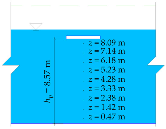
Figure 11.
Vertical position of the numerical probes for the WEC function.
4. Results and Discussion
Here, the results obtained for the verification and validation of the computational model for regular and irregular waves are presented, as well as the result of the verification performed with the OCEANLYZ software. Besides that, the results of the case study considering the SHP as breakwater and WEC when submitted to representative regular or realistic irregular waves from the sea state of Rio Grande are also reported.
4.1. Verification and Validation Results
4.1.1. Verification of the WaveMIMO Methodology
Figure 12 depicts the water free surface elevation result numerically obtained at x = 50 m with the WaveMIMO methodology for the representative regular waves of the Rio Grande coast, confronted with the analytical solution found through Equation (5). To facilitate visualization, the total simulation time of 300 s has been subdivided every 100 s, as can be noted in Figure 12a–c.
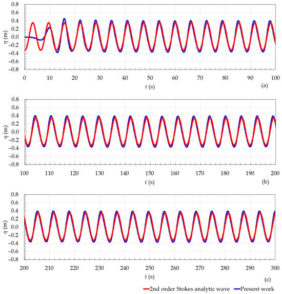
Figure 12.
Free surface elevation of representative regular waves of the Rio Grande sea state, considering (a) ; (b) ; and (c) 20.
In qualitative terms, as in [20,62,63], it can be seen that the WaveMIMO methodology adequately reproduces the representative regular waves. It should be noted that the greatest differences occur for due to the initial condition of fluid inertia, which is at rest at the beginning of the numerical simulation. Thus, quantitatively, the analysis of results considers the time interval 20, achieving MAE of 0.090 m and RMSE of 0.116 m. These results are in line with those found by [20,62,63].
After that, an analogous procedure was adopted to verify the irregular wave generation. Figure 13a,b shows the water free surface elevation for the realistic irregular waves of the Rio Grande sea state at x = 0 m (inlet region) in comparison with the results from TOMAWAC, respectively, in intervals of 300 s.
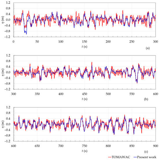
Figure 13.
Free surface elevation of realistic irregular waves, considering (a) ; (b) ; and (c) 60.
One can note that, qualitatively, the results of Figure 13 satisfactorily represent the random variation of the free surface elevation of the waves. During the 900 s taken into account in this analysis, MAE of 0.117 m and RMSE of 0.152 m were found. It stands out that the qualitative and quantitative results are consistent with those found by [62,64,65].
Based on the results of Figure 12 and Figure 13 and in the qualitative and quantitative evaluations carried out, it is possible to infer that the computational model employing the WaveMIMO methodology was verified for the numerical generation of regular and irregular waves from a sea state. It is worth mentioning that further details about verification and validation of the WaveMIMO can be found in Machado et al. [20] and Maciel et al. [63].
4.1.2. Validation of the Computational Model in a Laboratory Scale with SHP
Just as observed in the studies of Dick and Brebner [25], Graw [26], and Orer and Ozdamar [36], Figure 14 shows the pulsating effect of the axial velocity below the SHP obtained in the present work during wave propagation. This effect has led to further research into SHP as a WEC. As can be seen, the velocity is approximately zero up to t = 10 s. This is due to the time it takes for the first wave to propagate from the generation zone to the center of the SHP, since the initial condition of the fluid is rest.
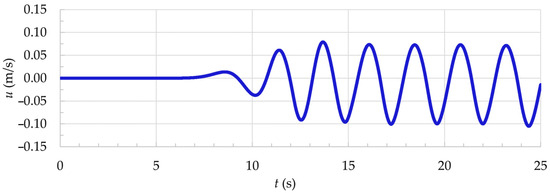
Figure 14.
Axial velocity pulsating effect under the SHP.
Table 4 shows a comparison of the maximum axial velocity found in the present study (from Figure 14 and through the WaveMIMO methodology) with that found in the experimental study by Orer and Ozdamar [36]. As presented in the literature [7,36,43], the pulsating flow below the SHP has its highest values in the opposite direction to the propagation, therefore, the results are presented with a negative value. Considering the RPE, Equation (14), the error between the numerical results obtained in this study and the experimental results by Orer and Ozdamar [36] is 7.73%, due to a difference of −0.0088 m/s. Therefore, it is considered that the computational model has been properly validated.
Table 4.
Computational model validation results.
4.1.3. Verification of the Full-Scale Computational Model with SHP
This evaluation was carried out by comparing the results obtained here by means of the WaveMIMO methodology with those reported by Seibt et al. [7]. To this end, due to the initial condition of fluid inertia, the analysis considers the interval between 25 s 104 s. Figure 15 shows, qualitatively, that the elevation of the water free surface monitored at the position of x = 104.688 m is properly reproduced. The quantitative analysis took into account Equations (12) and (13), where the differences for the free surface elevation were MAE of 0.030 m and RMSE of 0.040 m. Figure 16 also shows adequate reproduction of the axial velocity monitored below the SHP. Quantitatively, differences of 0.061 m/s and 0.077 m/s were observed for MAE and RMSE, respectively. Given the qualitative and quantitative results found in both analyses carried out, the numerical model is considered to be verified.
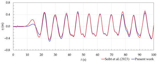
Figure 15.
Free surface elevation in x = 104.688 m for verification, Seibt et al. [7].
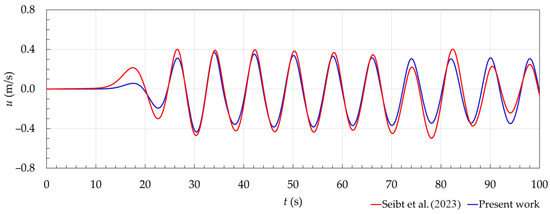
Figure 16.
Axial velocity below SHP at x = 141.911 m; z = 5.616 m for verification, Seibt et al. [7].
4.1.4. Verification of the OCEANLYZ Software
The last verification is addressed to show the applicability of the OCEANLYZ software in calculation of the Hs of waves. Then, it was applied in the free surface elevation data obtained by Equation (5) for the representative regular waves (see Figure 6). The result reached by the OCEANLYZ software was Hs = 0.66997 m, which in comparison with the Hs = 0.66 m has a RPE = 1.51%. It is therefore understood that the OCEANLYZ software is verified and adequately determines the value of the significant height for the data series in this study.
4.2. Results from the Case Study
As stated in this paper, the case study evaluates 5 different lengths of the SHP, with the aim of understanding the effects of this variation when the SHP is considered as a breakwater and when it is considered as a WEC. To do so, numerical simulations are performed of these 5 SHPs when submitted to the incidence of the representative regular and realistic irregular waves from the sea state of Rio Grande city. The influence of other important constructive (such as the SHP submergence depth) and operational (such as the incidence of different sea states) parameters was not evaluated in the present study but will be addressed in future investigations.
As for the analysis of the results, when the SHP is considered as a breakwater, the significant wave heights upstream and downstream of the SHP are compared. When the SHP is considered as WEC, the analysis is carried out by determining the maximum axial velocity occurring under the SHP. It is noteworthy that the SHP can be considered a WEC due to the axial velocity having positive and negative signs, indicating that the flow under the SHP occurs in an alternating way, a fact that is in agreement with other authors [7,36,42,43] and already reproduced here in Figure 14 and Figure 16.
4.2.1. SHP under the Incidence of the Representative Regular Waves
The characteristics of the representative regular waves can be seen in Figure 6. Due to the initial resting condition of the fluid, as previously mentioned, together with the stabilization of the regular waves, the time range under consideration is 20.
Concerning the evaluation of the SHP as breakwater, Figure 17a–e compares the results of the free surface elevation upstream and downstream of the SHP for each of the cases.
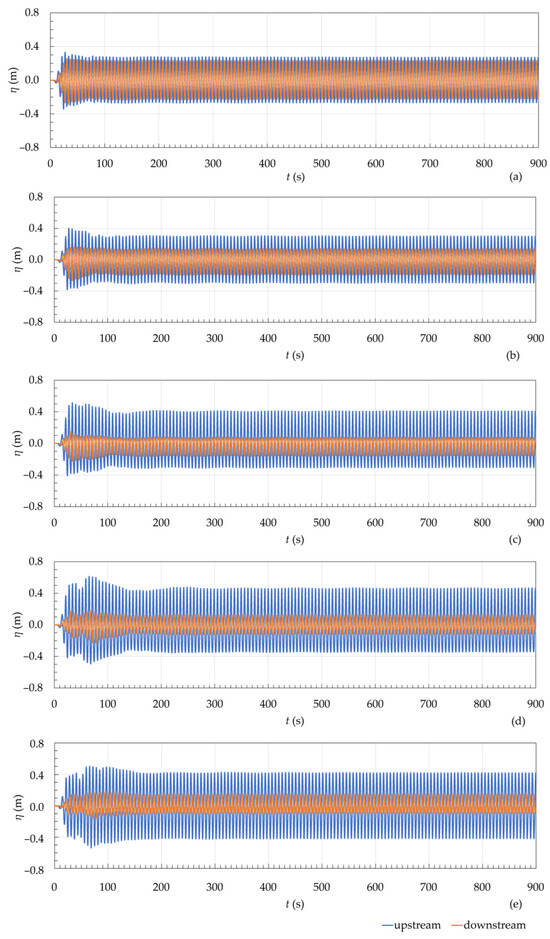
Figure 17.
Analysis of the SHP as a breakwater under representative regular waves: (a) 1Lp; (b) 1.5Lp; (c) 2Lp; (d) 2.5Lp; and (e) 3Lp.
Qualitatively, it can be seen in Figure 17 that there is a reduction of Hs for all cases, demonstrating consistency with SHP’s initial interest in reducing waves. It can also be seen that the reduction in free surface elevation after SHP is directly proportional to the length of the plate, with the 1Lp case showing the highest significant wave height downstream of the device. Therefore, quantitative analysis of the results is necessary to confirm this first visual impression.
Table 5 shows the results of Hs for all cases in the probes 10 m upstream and downstream of the SHP. The last column shows the RPE value between the probes in each case, i.e., the percentage reduction after propagation over the device.
Table 5.
Hs calculated at 10 m upstream and downstream of the SHP.
One can observe in Table 5 that the augmentation of the SHP length improves its effect as a breakwater, since between cases 1Lp and 3Lp a reduction superior to 55% was reached.
Next, a second way of evaluating the SHP in the breakwater function is presented. To do this, in all the cases evaluated (1Lp, 1.5Lp, 2Lp, 2.5Lp, and 3Lp), a probe was used to monitor the elevation of the free surface positioned at x = 128.63 m. Because this probe is further away from the SHP compared to the previous analysis and positioned before the start of the numerical beach, it is interpreted that these would be the significant wave heights that would reach the coast after passing through the device. Table 6 shows the quantitative comparison of Hs obtained from the probes located upstream and downstream of the SHP.
Table 6.
Hs considering the probe located 10 m upstream of the SHP and the fixed probe, at x = 128.63 m.
From Table 6, the results obtained for the 1Lp case show the efficiency of the device’s application as a breakwater under the incidence of representative regular waves. It has also been observed that the 3Lp case increased Hs reduction capacity by 5 times compared with the initial case. In contrast to the previous analysis, when comparing the significant height of the waves upstream of the SHP with the waves that reach the coast after passing through the device, the 2.5Lp case is the most efficient.
An interesting behavior is related to the efficiency increase in Hs reducing by approximately 3 times for the 1.5Lp case compared to the 1Lp case; whereas the Hs reduction of the best cases (2.5Lp and 3Lp) increased the efficiency around 4.5 times if compared with the worst one (1Lp). It is therefore understood that the variation in wave height reduction effects due to the length of the SHP is not linear, even in regular wave propagation.
Another point to discuss is the affordability of a long SHP. When comparing the Hs values that reach the coast for cases 2.5Lp and 3Lp, for example, the 20% increase in device length for the second case led to a decrease in wave height reduction efficiency. Therefore, given the nonlinear evolution of wave reduction efficiency, the interest in the behavior of SHP under the incidence of realistic irregular waves is greater.
Finally, one can highlight in Table 5 and Table 6 that the case 2Lp reaches percentage Hs reduction almost as large as the maximum values. In other words, it is possible to employ the SHP with 2Lp that is 50% smaller (see Table 5) and 25% smaller (see Table 6) than the best cases, with a difference of only 2.54% and 5.64%, respectively, in its efficiency as breakwater.
In sequence, the SHP was evaluated as a WEC when submitted to the representative regular waves of the Rio Grande sea state. Figure 18 shows the maximum axial velocity profiles obtained below the SHP along the depth (see Figure 11) for each of the cases. As mentioned, the maximum values are negative because the highest velocities occur in the opposite direction to wave propagation. This pattern is repeated in this study, as well as in the literature [36,42,43].
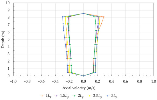
Figure 18.
Maximum axial velocity profiles over depth for the representative regular waves.
From Figure 18, one can observe that the 2.5Lp and 3Lp cases have a similar velocity profile in the direction of wave propagation, while for the maximum negative axial velocities, the case 3Lp achieves the highest velocity magnitudes among all cases. It can also be seen in Figure 18 that for the 1.5Lp and 2Lp cases, there were no considerable differences in the velocity profiles in the direction opposite to propagation. On the other hand, in the positive direction, there is a variation when approaching the bottom of the SHP. However, in this study, the region of interest for the future installation of a turbine is the midpoint between the bottom of the SHP and the bottom of the wave channel, as in [7,36,39,41,42]. This point of interest has its horizontal coordinate located at the center of the SHP and the vertical coordinate at z = 4.284 m. It should be noted that, as the SHP lengths investigated were different, the horizontal coordinate (x) has a specific value in each case. Thereby, Table 7 shows the maximum axial velocity calculated at the point of interest for each case.
Table 7.
Maximum axial velocity at position z = 4.284 m and time of occurrence for the representative regular waves.
As already noticed in Figure 18, Table 7 indicates that the highest axial velocity was found for the 3Lp case, which means that, among the SHP dimensions evaluated, it had the greatest potential for converting the energy contained in sea waves into electricity. The 3Lp case had the maximum negative axial velocity 5.41% bigger than the 1Lp case; remembering that the 1Lp case has the dimensions optimized for a regular wave from the 2nd order Stokes theory by Seibt et al. [7]. The worst case found is the 2Lp, which has a conversion potential 25.43% lower than the best case, 3Lp.
Figure 19 displays the axial velocity variation for all cases over time at the point of interest. Qualitatively, the pulsating effect of velocity below SHP is visible for all cases, as presented in the verification and validation procedures and in the reference studies of Orer and Ozdamar [36] and Seibt et al. [7]. The variation in the amplitude of these axial velocities between each case is noticeable, demonstrating that the maximum results of each case are regular over time and not an isolated extreme value.
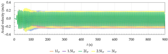
Figure 19.
Axial velocities at the point of interest over time.
4.2.2. SHP under the Incidence of the Irregular Realistic Waves
This section presents the results obtained when the SHP was subjected to the incidence of the realistic irregular waves and considered both as a breakwater and as a WEC. Due to the random behavior of the irregular waves, the entire period of wave generation and propagation is taken into account in the qualitative and quantitative analyses, i.e., the results presented in this section correspond to a series of 900 s.
For the SHP acting as a breakwater, Figure 20 illustrates the free surface elevation of the waves monitored by the probes located 10 m upstream (fixed probes at x = 93.2 m) from the SHP and 10 m downstream (variable probe) from the SHP. Qualitatively, in all five cases, the free surface elevation obtained upstream of the SHP is higher than that obtained downstream of the SHP. This is consistent with the physical principle of a breakwater, which is to reduce the wave height downstream.
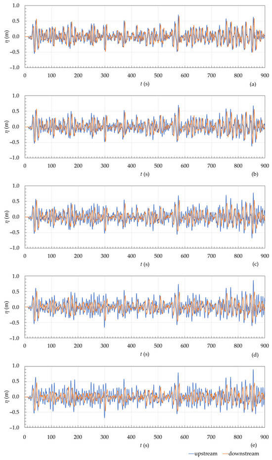
Figure 20.
Analysis of the SHP as a breakwater under realistic irregular waves: (a) 1Lp; (b) 1.5Lp; (c) 2Lp; (d) 2.5Lp; and (e) 3Lp.
In turn, Table 8 reports the quantitative results obtained for the Hs when considering the probes 10 m upstream and downstream of the SHP, as well as the percentage of Hs reduction after the propagation of the realistic irregular waves over the device. As with the previous results, the 3Lp case was the one with the greatest Hs reduction, in short, it demonstrated the greatest efficiency as the breakwater. Furthermore, when comparing the most and least efficient cases, 3Lp and 1Lp, respectively, there was a difference in the damping of the significant wave height of approximately 8 times. Also, the Hs reduction in this comparison was directly proportional to the length of the SHP, i.e., the longer the SHP, the greater the reduction was. The same trend was observed in Table 5 for the representative regular waves.
Table 8.
Hs calculated upstream and downstream of SHP.
As can be seen in Table 8, the Hs reduction in the 1Lp case was negligible for this analysis of the SHP under realistic irregular waves. In contrast, the Hs reduction in the regular wave analysis showed fair results (see Table 5 and Table 6). Therefore, evaluations of the effects of different SHP characteristics on the device as a breakwater under realistic irregular waves are justified.
For the reduction of waves by a breakwater, dimensional parameters of the geometry such as plate length, thickness, and installation depth ratio can be important, as presented by the literature considering regular waves [7,28,32,33,39,41,42,44]. The authors chose to start the investigation varying the length Lp, because, in proportion to the incident representative regular waves, the plate in case 1Lp was too “short” for the wavelength (1Lp = 3.457 m versus λ = 51.6 m). This fact indicated a first path to understanding the relevance of the SHP length on the influence of its efficiency as a breakwater. The authors’ choice led to creating the 4 other cases investigated in this work.
As in the previous study, a second assessment of the SHP as a breakwater is presented below, based on an analysis of the free surface elevations obtained using a probe fixed at the downstream position x = 128.63 m in all cases. As before, these are the free surface elevations of the waves that reach the coast after passing the SHP. Therefore, Table 9 shows and compares the Hs obtained through the fixed probes located in the horizontal coordinates x = 93.2 m and x = 128.63 m, respectively, upstream and downstream of the SHP.
Table 9.
Hs considering the probe located 10 m upstream of the SHP and the fixed downstream probe, located at x = 128.63 m.
From Table 9, the result of the 1Lp case reveals poor efficiency in the application of the device as a breakwater under the incidence of realistic irregular waves, as also noticed in Table 8. However, there was a significant increase in device efficiency when 1.5Lp SHP was considered. Moreover, when comparing the cases with the highest and lowest efficiency, 3Lp and 1Lp, respectively, the difference in wave damping was more than 19 times. Finally, it is important to note that when considering realistic irregular waves, unlike representative regular waves, the greater damping of the Hs occurred for the 3Lp case regardless of the position of the downstream probe.
An interesting fact is that for the realistic irregular wave situation, for both probes downstream of the SHP, the efficiency was less than 40% (see Table 8 and Table 9). In the case of representative regular waves, however, only case 1Lp had an efficiency of less than 40% for both downstream probes (see Table 5 and Table 6). It can therefore be seen that there is a wide variation in the effects of the length of the SHP as a breakwater for the different wave approaches. This result, which calls for further investigations, shows the gap between the theoretical values of regular waves and what actually happens with irregular waves on the ocean and coasts.
Both in the case of representative regular waves and realistic irregular waves, it was not possible to determine a pattern to the changes in efficiency in relation to the probe 10 m downstream and the fixed probe after the SHP. This consideration has led to questions about the evolution of the wave during propagation after the SHP.
In the situation of realistic irregular waves, there is no proximity between the values of the efficiency in the reduction of Hs for each case, unlike the results for regular waves. For realistic irregular waves, these differences between the cases 2.5Lp and 3Lp are 7.11% for the probe 10 m downstream of the SHP (see Table 8) and 10.09% for the fixed probe after the device (see Table 9). However, in the approach with the representative regular waves, the variation in reductions was less than 2% when comparing the same cases for both probes after SHP (see Table 5 and Table 6).
Finally, concerning the SHP as a WEC under the incidence of the realistic irregular waves, Figure 21 shows the maximum axial velocity profiles obtained below the SHP along the depth (see Figure 11) for each of the cases. As mentioned, the maximum values are negative due to the fact that the highest velocities occur in the opposite direction to wave propagation. This pattern presented in the literature for regular waves [36,42,43] is repeated in these results for the SHP under realistic irregular waves. The pulsating effect of the flow also occurred in these cases. This can be seen in Figure 21, which shows the maximum axial velocities in the positive and negative directions. However, this pulsating flow is irregular, and so are the free surface elevations.
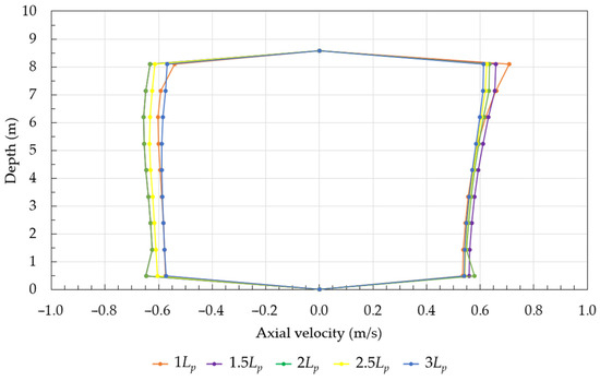
Figure 21.
Maximum axial velocity profiles over depth for the realistic irregular waves.
Among all the depths evaluated, the maximum axial velocities were obtained for the 2Lp case. In turn, when comparing the maximum axial velocities obtained with 1.5Lp and 2Lp, it was clear that there were no considerable differences in the velocities obtained along the depth; the same occurred when comparing cases 1Lp and 3Lp. Then, comparing the case with the lowest maximum axial velocities, 3Lp, with the case showing the highest velocities, 2Lp, there was an average reduction in velocity of 9%.
As already identified in the results depicted in Figure 21, Table 10 shows the maximum axial velocity calculated at the point of interest when considering the random waves. The smallest axial velocity was found for the 3Lp case, that is, among the dimensions of the SHP evaluated, it is the one with the least potential for converting the energy contained in sea waves into electricity, while the case with the highest maximum axial velocity is 2Lp. Comparing the worst and best performing cases, one can note that the 2Lp case has a conversion potential around 9% higher than the 3Lp case.
Table 10.
Maximum axial velocity at point of interest and time of occurrence for the realistic irregular waves.
5. Conclusions
This numerical study investigated different lengths of SHP subjected to representative regular waves and realistic irregular waves of the sea state that occurred on the coast of the city of Rio Grande in southern Brazil. In addition, the SHP was evaluated in terms of breakwater and WEC functionalities. To do so, the computational model employing the WaveMIMO methodology was validated and verified.
As a breakwater and under the incidence of the representative regular waves, with the exception of the 1Lp case, the cases showed an efficiency of more than 40% in the reduction of Hs downstream from the device. Considering the downstream probe fixed at x = 128.63 m and interpreting the significant wave heights as those that reach the shore after passing through the device, the 2.5Lp case had the best performance. In turn, when the SHP was considered as a WEC and submitted to the representative regular waves, the best performance was achieved by the 3Lp case, with the average maximum axial velocity along the depth being 25% higher than the case with the lowest velocities. The pulsating effect of the flow below the SHP was also demonstrated, in agreement with other studies in the literature already mentioned [7,26,36,39,42].
On the other hand, for the evaluation involving the realistic irregular waves, the SHP as a breakwater obtained efficiencies in the Hs reducing less than 40% for all analyzed cases. Here, the SHP length proved to be an important parameter: considering the fixed probe and interpreting it as the value of Hs that reaches the coast, the 1Lp case had a negligible efficiency of 1.98% in reducing the incident wave heights; while the 3Lp case achieved 38.28% in the Hs reduction, being the more efficient breakwater among the investigated cases. In other words, when comparing the most and least efficient cases, i.e., 3Lp and 1Lp, respectively, there was a difference of approximately 19 times in the damping of the wave heights reaching the shore. Besides that, the SHP as WEC and submitted to the realistic irregular waves showed the highest maximum axial velocities for all the depths evaluated in the case of 2Lp, presenting an average increase of 9% in relation to the case 3Lp, which had the lowest velocities.
This paper concludes with two findings: (a) confirmation that the use of regular waves in numerical studies is insufficient to determine the real hydrodynamics of the process, especially if the focus is to define the efficiency of the SHP as breakwater and/or as WEC; (b) these results are the very first ones to numerically consider the SHP with irregular waves and considering both functions as breakwater and as WEC. There is still a need for better understanding of the SHP as a breakwater and the effects of plate length on wave propagation after the device, since there were variations in the efficiency for the cases 2.5Lp and 3Lp between the probes 10 m downstream of the device and on the downstream fixed probe. For the SHP as WEC, the most efficient lengths were different for each wave situation; the 3Lp case showed the highest axial velocity for representative regular waves while the 2Lp case was the one with the highest conversion capacity for realistic irregular waves.
Finally, based on the obtained results, one can infer that the SHP with 3Lp length should be chosen to meet the needs as breakwater and the SHP with 2Lp length as WEC, as these lengths are the most appropriate and with good efficiency level in each function.
In addition, there is a clear need to expand the investigations of the SHP device with sea states, bringing the efficiencies closer to the real situation in which the device is installed, as well as an investigation between the lengths of the cases 2Lp and 3Lp, aiming to refine the search for the best SHP for both functions. Furthermore, an investigation with higher values for the SHP length is also relevant in order to identify to what extent the observed trend persists. In addition, other important constructive parameters, such as the submergence depth, will be evaluated under the incidence of irregular waves. These aspects should be the focus of future studies into the development of SHP with the integration of breakwater and WEC functions.
Author Contributions
Conceptualization, G.Ü.T., B.N.M. and L.A.I.; methodology, G.Ü.T., R.P.M., P.H.O., B.N.M. and L.A.I.; software, G.Ü.T., R.P.M. and P.H.O.; validation, G.Ü.T., R.P.M., P.H.O. and F.M.S.; formal analysis, G.Ü.T., L.A.O.R., E.D.d.S., F.M.S., B.N.M. and L.A.I.; investigation, G.Ü.T., B.N.M. and L.A.I.; resources, L.A.O.R., E.D.d.S., B.N.M. and L.A.I.; data curation, G.Ü.T., R.P.M., P.H.O. and F.M.S.; writing—original draft preparation, G.Ü.T.; writing—review and editing, G.Ü.T., B.N.M. and L.A.I.; visualization, L.A.O.R., E.D.d.S., F.M.S., B.N.M. and L.A.I.; supervision, B.N.M. and L.A.I.; project administration, L.A.I.; funding acquisition, L.A.O.R., E.D.d.S., B.N.M. and L.A.I. All authors have read and agreed to the published version of the manuscript.
Funding
CAPES (Coordination for the Improvement of Higher Education Personnel—Brazil, funding code 001); CNPq (National Council for Scientific and Technological Development—Brazil, processes: 307791/2019-0, 308396/2021-9, 309648/2021-1, and 403408/2023-7); and FAPERGS (Foundation for the Support of Research in the State of Rio Grande do Sul—Brazil, process: 21/2551-0002231-0).
Data Availability Statement
The data presented in this study are available on request from the corresponding author. The data are not publicly available due to privacy reasons.
Acknowledgments
G. Ü. Thum thanks CAPES for the master’s scholarship (funding code 001). L. A. O. Rocha, E. D. dos Santos, and L. A. Isoldi thank CNPq for their research productivity grants (processes: 307791/2019-0, 308396/2021-9, and 309648/2021-1, respectively). The authors would also like to thank CNPq (Call CNPq/MCTI N° 10/2023—Universal, Process: 403408/2023-7), FAPERGS (Public Call 07/2021—Programa Pesquisador Gaúcho—PqG, process: 21/2551-0002231-0), and UFRGS (Edital PROPESQ/UFRGS 2019—Programa Institucional de Auxílio à Pesquisa de Docentes Recém-Contratados pela UFRGS) for their financial support.
Conflicts of Interest
The authors declare no conflicts of interest. The funders had no role in the design of the study; in the collection, analyses, or interpretation of data; in the writing of the manuscript; or in the decision to publish the results.
References
- United Nations Framework Convention on Climate Change. Paris Agreement. In Proceedings of the Conference of Parties 17; United Nations Framework Convention on Climate Change: Paris, France, 2015; p. 32. Available online: https://unfccc.int/process-and-meetings/the-paris-agreement (accessed on 13 July 2024).
- United Nations. Transforming Our World: The 2030 Agenda for Sustainable Development. Resolution Adopted by the General Assembly on 25 September 2015. Available online: https://www.un.org/en/development/desa/population/migration/generalassembly/docs/globalcompact/A_RES_70_1_E.pdf (accessed on 13 July 2024).
- González, A.T.; Dunning, P.; Howard, I.; McKee, K.; Wiercigroch, M. Is Wave Energy Untapped Potential? Int. J. Mech. Sci. 2021, 205, 106544. [Google Scholar] [CrossRef]
- UNESCO. The Science We Need for the Ocean We Want: Report; Intergovernmental Oceanographic Commission: Paris, France, 2019; Available online: https://en.unesco.org/news/science-we-need-ocean-we-want (accessed on 13 July 2024).
- Tavakoli, S.; Khojasteh, D.; Haghani, M.; Hirdaris, S. A Review on the Progress and Research Directions of Ocean Engineering. Ocean Eng. 2023, 272, 113617. [Google Scholar] [CrossRef]
- Wahyudie, A.; Jama, M.A.; Susilo, T.B.; Saeed, O.; Nandar, C.S.A.; Harib, K. Simple Bottom-up Hierarchical Control Strategy for Heaving Wave Energy Converters. Int. J. Electr. Power Energy Syst. 2017, 87, 211–221. [Google Scholar] [CrossRef]
- Seibt, F.M.; Dos Santos, E.D.; Isoldi, L.A.; Rocha, L.A.O. Constructal Design on Full-Scale Numerical Model of a Submerged Horizontal Plate-Type Wave Energy Converter. Mar. Syst. Ocean Technol. 2023, 18, 1–13. [Google Scholar] [CrossRef]
- Espindola, R.L.; Araújo, A.M. Wave Energy Resource of Brazil: An Analysis from 35 Years of ERA-Interim Reanalysis Data. PLoS ONE 2017, 12, e0183501. [Google Scholar] [CrossRef] [PubMed]
- Dias, F.; Dutykh, D.; Ghidaglia, J.-M. A two-fluid model for violent aerated flows. Comput. Fluids 2010, 39, 283–293. [Google Scholar] [CrossRef]
- Kim, S.P. CFD as a seakeeping tool for ship design. Int. J. Nav. Archit. Ocean Eng. 2011, 3, 65–71. [Google Scholar] [CrossRef]
- Dutykh, D.; Poncet, R.; Dias, F. The VOLNA code for the numerical modeling of tsunami waves: Generation, propagation and inundation. Eur. J. Mech. B Fluids 2011, 30, 598–615. [Google Scholar] [CrossRef]
- Rafiee, A.; Dutykh, D.; Dias, F. Numerical Simulation of Wave Impact on a Rigid Wall Using a Two–phase Compressible SPH Method. Procedia IUTAM 2015, 18, 123–137. [Google Scholar] [CrossRef]
- Wang, J.; Wan, D. CFD Investigations of Ship Maneuvering in Waves Using naoe-FOAM-SJTU Solver. J. Marine. Sci. Appl. 2018, 17, 443–458. [Google Scholar] [CrossRef]
- Liu, S.; Gatin, I.; Obhrai, C.; Ong, M.C.; Jasak, H. CFD simulations of violent breaking wave impacts on a vertical wall using a two-phase compressible solver. Coast. Eng. 2019, 154, 103564. [Google Scholar] [CrossRef]
- Jiao, J.; Huang, S.; Guedes Soares, C. Viscous fluid–flexible structure interaction analysis on ship springing and whipping responses in regular waves. J. Fluids Struct. 2021, 106, 103354. [Google Scholar] [CrossRef]
- Liu, B.; Park, S. CFD Simulations of the Effects of Wave and Current on Power Performance of a Horizontal Axis Tidal Stream Turbine. J. Mar. Sci. Eng. 2023, 11, 425. [Google Scholar] [CrossRef]
- Amini, M.; Memari, A.M. CFD Evaluation of Regular and Irregular Breaking Waves on Elevated Coastal Buildings. Int. J. Civ. Eng. 2024, 22, 333–358. [Google Scholar] [CrossRef]
- Liao, X.-Y.; Xia, J.-S.; Chen, Z.-Y.; Tang, Q.; Zhao, N.; Zhao, W.-D.; Gui, H.-B. Application of CFD and FEA Coupling to Predict Structural Dynamic Responses of a Trimaran in Uni- and Bi-Directional Waves. China Ocean Eng. 2024, 38, 81–92. [Google Scholar] [CrossRef]
- Opoku, F.; Uddin, M.N.; Atkinson, M. A Review of Computational Methods for Studying Oscillating Water Columns—The Navier-Stokes Based Equation Approach. Renew. Sustain. Energy Rev. 2023, 174, 113124. [Google Scholar] [CrossRef]
- Machado, B.N.; Oleinik, P.H.; de Paula Kirinus, E.; Rocha, L.A.O.; das Neves Gomes , M.; Conde, J.M.P.; Isoldi, L.A. WaveMIMO Methodology: Numerical Wave Generation of a Realistic Sea State. J. Appl. Comput. Mech. 2021, 7, 2129–2148. [Google Scholar] [CrossRef]
- Muehe, D. Erosão E Progradação Do Litoral Brasileiro; Ministério do Meio Ambiente: Brasília, Brazil, 2006. [Google Scholar]
- Trombetta, T.B.; Marques, W.; Guimarães, R.C.; Kirinus, E.D.P.; Silva, D.V.D.; Oleinik, P.H.; Leal, T.F.; Isoldi, L.A. Longshore Sediment Transport on the Brazilian Continental Shelf. Sci. Plena 2019, 15. [Google Scholar] [CrossRef]
- Heins, A.E. Water Waves Over a Channel of Finite Depth with a Submerged Plane Barrier. Can. J. Math. 1950, 2, 210–222. [Google Scholar] [CrossRef]
- Greene, T.R.; Heins, A.E. Water Waves Over a Channel of Infinite Depth. Appl. Math. 1953, XI, 201–214. [Google Scholar] [CrossRef]
- Dick, T.M.; Brebner, A. Solid and Permeable Submerged Breakwaters. In Coastal Engineering; American Society of Civil Engineers: London, UK, 1968; pp. 1141–1158. [Google Scholar]
- Graw, K. Is the Submerged Plate Wave Energy Converter Ready to Act as a New Coastal Protection System? In Proceedings of the XXIV Convegno Di Idraulica e Costruzioni Idrauliche, Napoli, Italy, 20–22 September 1994. [Google Scholar]
- Lima, S.F.; Almeida, L.E.; Toldo, E., Jr. Estimativa da Capacidade de Transporte Longitudinal de Sedimentos a partir de Dados de Ondas para a Costa do Rio Grande do Sul. Pesqui. Em Geociências 2001, 28, 99. [Google Scholar] [CrossRef]
- Yu, X. Functional Performance of a Submerged and Essentially Horizontal Plate for Offshore Wave Control: A Review. Coast. Eng. J. 2002, 44, 127–147. [Google Scholar] [CrossRef]
- Hayatdavoodi, M.; Ertekin, R.C.; Valentine, B.D. Solitary and Cnoidal Wave Scattering by a Submerged Horizontal Plate in Shallow Water. AIP Adv. 2017, 7, 065212. [Google Scholar] [CrossRef]
- Karmakar, D.; Soares, C.G. Wave Motion Control Over Submerged Horizontal Plates. In Proceedings of the ASME 2015 34th International Conference on Ocean, Offshore and Arctic Engineering, St. John’s, NL, Canada, 31 May–5 June 2015. [Google Scholar]
- Siew, P.F.; Hurley, D.G. Long Surface Waves Incident on a Submerged Horizontal Plate. J. Fluid. Mech. 1977, 83, 141–151. [Google Scholar] [CrossRef]
- Wang, K.-H.; Shen, Q. Wave Motion over a Group of Submerged Horizontal Plates. Int. J. Eng. Sci. 1999, 37, 703–715. [Google Scholar] [CrossRef]
- Cheng, Y.; Ji, C.; Ma, Z.; Zhai, G.; Oleg, G. Numerical and Experimental Investigation of Nonlinear Focused Waves-Current Interaction with a Submerged Plate. Ocean Eng. 2017, 135, 11–27. [Google Scholar] [CrossRef]
- Fang, Q.; Yang, C.; Guo, A. Hydrodynamic Performance of Submerged Plates During Focused Waves. J. Mar. Sci. Eng. 2019, 7, 389. [Google Scholar] [CrossRef]
- Aghili, M.; Ghadimi, P.; Faghfoor Maghrebi, Y.; Nowruzi, H. Simulating the Interaction of Solitary Wave and Submerged Horizontal Plate Using SPH Method. Int. J. Phys. Res. 2014, 2, 16–26. [Google Scholar] [CrossRef][Green Version]
- Orer, G.; Ozdamar, A. An Experimental Study on the Efficiency of the Submerged Plate Wave Energy Converter. Renew. Energy 2007, 32, 1317–1327. [Google Scholar] [CrossRef]
- Wagner, J.J.; Wagner, J.R.; Hayatdavoodi, M. Hydrodynamic analysis of a submerged wave energy converter. In Proceedings of the 4th Marine Energy Technology Symposium METS2016, Washington, DC, USA, 25–27 April 2016. [Google Scholar]
- Xu, Y.; Zhang, G.; Wan, D.; Chen, G. MPS Method for Study of Interactions between Solitary Wave and Submerged Horizontal Plate. In Proceedings of the 29th International Ocean and Polar Engineering Conference, Honolulu, HI, USA, 16–21 June 2019. [Google Scholar]
- Seibt, F.M.; Couto, E.C.; Dos Santos, E.D.; Isoldi, L.A.; Rocha, L.A.O.; Teixeira, P.R.D.F. Numerical Study on the Effect of Submerged Depth on the Horizontal Plate Wave Energy Converter. China Ocean Eng. 2014, 28, 687–700. [Google Scholar] [CrossRef]
- Carter, W.R. Wave Energy Converters and A Submerged Horizontal Plate. Master’s Thesis, Ocean and Resources Engineering, University of Hawaii, Honolulu, HI, USA, 2005. [Google Scholar]
- Seibt, F.M.; Couto, E.C.; Teixeira, P.R.D.F.; Dos Santos, E.D.; Rocha, L.A.O.; Isoldi, L.A. Numerical Analysis of the Fluid-Dynamic Behavior of a Submerged Plate Wave Energy Converter. Comput. Therm. Sci. Int. J. 2014, 6, 525–534. [Google Scholar] [CrossRef]
- Seibt, F.; De, C.; Dos, S.; Das, N.; Rocha, L.; Isoldi, L.; Fragassa, C. Numerical Evaluation on the Efficiency of the Submerged Horizontal Plate Type Wave Energy Converter. FME Trans. 2019, 47, 543–551. [Google Scholar] [CrossRef]
- He, M.; Gao, X.; Xu, W.; Ren, B.; Wang, H. Potential Application of Submerged Horizontal Plate as a Wave Energy Breakwater: A 2D Study Using the WCSPH Method. Ocean Eng. 2019, 185, 27–46. [Google Scholar] [CrossRef]
- Zheng, Y.; Zhou, Y.; Jin, R.; Mu, Y.; He, M.; Zhao, L. Experimental Study on Submerged Horizontal Perforated Plates under Irregular Wave Conditions. Water 2023, 15, 3015. [Google Scholar] [CrossRef]
- Chakrabarti, S.K. Handbook of Offshore Engineering; Elsevier: Amsterdam, The Netherlands, 2005; Volume I, ISBN 978-0-08-044568-7. [Google Scholar]
- Dean, R.G.; Dalrymple, R.A. Water Wave Mechanics for Engineers and Scientists; Advanced Series on Ocean Engeneering; WSPC: Singapore, 1991; Volume 2, ISBN 981-02-0420-5. [Google Scholar]
- Samad, A.; Sannasiraj, S.A.; Sundar, V.; Halder, P. (Eds.) Ocean Wave Energy Systems: Hydrodynamics, Power Takeoff and Control Systems; Ocean Engineering & Oceanography; Springer International Publishing: Cham, Switzerland, 2022; Volume 14. [Google Scholar]
- Oleinik, P.H.; Tavares, G.P.; Machado, B.N.; Isoldi, L.A. Transformation of Water Wave Spectra into Time Series of Surface Elevation. Earth 2021, 2, 997–1005. [Google Scholar] [CrossRef]
- Holthuijsen, L.H. Waves in Oceanic and Coastal Waters; Cambridge University Press: New York, NY, USA, 2007. [Google Scholar]
- ANSYS, Inc. Ansys Fluent Theory Guide; ANSYS, Inc.: Canonsburg, PA, USA, 2013. [Google Scholar]
- Patankar, S.V. Numerical Heat Transfer and Fluid Flow; McGraw-Hill: New York, NY, USA, 1980. [Google Scholar]
- Versteeg, H.K.; Malalasekera, W. An Introduction to Computational Fluid Dynamics—The Finite Volume Method; Pearson Education Limited: London, UK, 2007. [Google Scholar]
- Schlichting, H. Boundary Layer Theory; McGraw-Hill: New York, NY, USA, 1979. [Google Scholar]
- Hirt, C.W.; Nichols, B.D. Volume of Fluid (VOF) Method for the Dynamics of Free Boundaries. J. Comp. Phys. 1981, 39, 201–225. [Google Scholar] [CrossRef]
- Gomes, M.D.N.; Lorenzini, G.; Rocha, L.A.O.; Santos, E.D.D.; Isoldi, L.A. Constructal Design Applied to the Geometric Evaluation of an Oscillating Water Column Wave Energy Converter Considering Different Real Scale Wave Periods. J. Eng. Thermophys. 2018, 27, 173–190. [Google Scholar] [CrossRef]
- Srinivasan, V.; Salazar, A.J.; Saito, K. Modeling the Disintegration of Modulated Liquid Jets Using Volume-of-Fluid (VOF) Methodology. Ap. Math. Mod. 2011, 3710–3730. [Google Scholar] [CrossRef]
- da Cruz Lisboa, R.; de Freita, T.P.R.; Eric, D. Simulação da propagação de ondas regulares e irregulares em um canal bidimensional com praia numérica. In Proceedings of the VII Seminário e Workshop em Engenharia Oceânica, Rio Grande, Brazil, 4 December 2016. [Google Scholar]
- Mavriplis, D.J. Unstructured Grid Techniques. Annu. Rev. Fluid. Mech. 1997, 29, 473–514. [Google Scholar] [CrossRef]
- Chai, T.; Draxler, R.R. Root Mean Square Error (RMSE) or Mean Absolute Error (MAE)?—Arguments against Avoiding RMSE in the Literature. Geosci. Model. Dev. 2014, 7, 1247–1250. [Google Scholar] [CrossRef]
- Kar, C.-J.; Els, P.S. Validation Metric Based on Relative Error. Math. Comput. Model. Dyn. Syst. 2012, 18, 487–520. [Google Scholar] [CrossRef]
- Karimpour, A. OCEANLYZ. Available online: https://github.com/akarimp/Oceanlyz (accessed on 13 July 2024).
- Maciel, R.P.; Oleinik, P.H.; Dos Santos, E.D.; Rocha, L.A.O.; Machado, B.N.; Gomes, M.D.N.; Isoldi, L.A. Constructal Design Applied to an Oscillating Water Column Wave Energy Converter Device under Realistic Sea State Conditions. J. Mar. Sci. Eng. 2023, 11, 2174. [Google Scholar] [CrossRef]
- Maciel, R.P.; Fragassa, C.; Machado, B.N.; Rocha, L.A.O.; Dos Santos, E.D.; Gomes, M.N.; Isoldi, L.A. Verification and Validation of a Methodology to Numerically Generate Waves Using Transient Discrete Data as Prescribed Velocity Boundary Condition. J. Mar. Sci. Eng. 2021, 9, 896. [Google Scholar] [CrossRef]
- Cisco, L.A.; Maciel, R.P.; Oleinik, P.H.; Dos Santos, E.D.; Gomes, M.N.; Rocha, L.A.O.; Isoldi, L.A.; Machado, B.N. Numerical Analysis of the Available Power in an Overtopping Wave Energy Converter Subjected to a Sea State of the Coastal Region of Tramandaí, Brazil. Fluids 2022, 7, 359. [Google Scholar] [CrossRef]
- Hubner, R.G.; Fragassa, C.; Paiva, M.D.S.; Oleinik, P.H.; Gomes, M.D.N.; Rocha, L.A.O.; Santos, E.D.D.; Machado, B.N.; Isoldi, L.A. Numerical Analysis of an Overtopping Wave Energy Converter Subjected to the Incidence of Irregular and Regular Waves from Realistic Sea States. J. Mar. Sci. Eng. 2022, 10, 1084. [Google Scholar] [CrossRef]


Disclaimer/Publisher’s Note: The statements, opinions and data contained in all publications are solely those of the individual author(s) and contributor(s) and not of MDPI and/or the editor(s). MDPI and/or the editor(s) disclaim responsibility for any injury to people or property resulting from any ideas, methods, instructions or products referred to in the content. |
© 2024 by the authors. Licensee MDPI, Basel, Switzerland. This article is an open access article distributed under the terms and conditions of the Creative Commons Attribution (CC BY) license (https://creativecommons.org/licenses/by/4.0/).