How to Compute Whether Biomass Fuels Are Carbon Neutral

Abstract

Based on recent interest and on the importance of the ongoing climate change catastrophe, this article provides the basics of global carbon cycle modelling as required for the assessment of the degree of carbon neutrality of biomass energy, and its underlying dynamics. It is aimed at clarifying the question “Are biomass fuels carbon neutral?”. The “Combined Energy and Biosphere Model” (CEBM) computes annual carbon flows including growth and decay of plants on 2.5 × 2.5° grid elements of the continents’ surface and offers detailed results on the changes of after implementation of large-scale biomass energy strategies worldwide. The main (and possibly unexpected) effect is the long-term depletion of the soil organic compartment after extraction of biomass fuels. When comparing CEBM model runs using (i) biomass energy sources and (ii) carbon-free energy sources (such as solar or wind), it becomes quantitatively clear already on the theoretical level (i.e., even without taking into account efficiency losses) that biomass is only “half as carbon neutral” as ideally assumed, to express a rule of thumb—mainly because of soil carbon depletion. Still, biomass energy will play an important role when fighting global warming, even if efforts to lower energy demand are preferable as a fundamental strategy.

1. Introduction

1.1. Motivation

In order to realistically fulfil the (existing and most urgently needed) global and national climate protection targets, all potential measures have to be implemented to a maximum extent. Within the European Union and adjacent countries, the recent “Green Deal” exerted a major wave of innovation [1,2,3] on the policy level. From among the available energy-related strategies, and given its immediate technological availability [4,5,6,7,8,9,10,11,12], biomass energy has been playing a key practical role for decades already, and was conceptually supported by the traditional assumption of its carbon neutrality: under sustainable conditions, carbon dioxide emitted during combustion was held to be equal to its absorption during plant growth [13,14,15,16,17,18,19,20]. However, in order to clarify conditions of carbon (C) neutrality quantitatively and more reliably [21,22,23,24,25,26,27,28,29,30,31,32,33,34], it became necessary to model the annual natural C cycle globally and to consider its changes as a result of steadily growing large-scale biomass strategies [35,36,37,38,39,40,41,42,43]. Because a recent publication [44] found much interest in readership [45,46,47,48,49,50,51,52,53,54,55], this article dwells still deeper into the dynamism of C flows and their alterations after biomass fuel extraction from the natural C cycle.

The present article contributes to solving the question: what type of global model do we need to assess whether biomass fuels are carbon neutral?

The aim of the study is to clarify the degree of carbon neutrality of biomass energy in practice for five different biomass cultivation modes, and to describe it quantitatively in space-time resolution.

Its key contribution is to model the alterations of the C cycle after biomass fuel use.

While there exist analyses for hypothetical geographical areas [56,57,58,59,60], now analysis of the entire surface is visible as of now. Also, this article combines energy modelling (including socio-economic scenarios) to biosphere modelling of the entire C cycle.

1.2. Relevance

Al efforts in the UNFCCC and IPCC frames and quite concretely, the recent “European Green Deal” [61] calls for quantification of the positive effect of various climate protection strategies on the CO₂ content in the atmosphere [62], including foresight methods [63]. The presented models offer support to achieve this goal. Especially because recent publications [44,64,65] receive interest ([48], p. 2), and the theme of biomass C neutrality is continuously discussed [66,67,68,69,70,71,72,73,74,75,76], the present article undertakes to dwell more into modelling details on the global carbon cycle.

What is already known in the open literature? As can be seen from these reference (and the in-depth analysis performed in [44]), a general conviction appears to exist that biomass energy is carbon-neutral. However, this latent conviction is almost never corroborated by model-based evidence. Often, the only reasons for reducing the degree of carbon neutrality seem to be secondary energy use for processing biomass-based fuels only. While these actually do reduce carbon-neutrality, they are not the only one and not the most important reason for biomass not fulfilling the high hopes set into them. This key effect, however, is an intrinsic effect of soil depletion which can only be analysed by a dynamic, time-and-space-resolved C cycle model as the one presented here.

What is missing (i.e., which research gaps remain in literature)? The effects of large-scale removal of plant matter from the biosphere on the carbon cycle after producing biomass energy has not yet been studied consistently. Therefore, the reduced input of plant matter into the humus layers of the soil remains unaccounted for in most cases. Therefore, the generic effects of depletion within the amount of soil organic matter do not show up in the perception—which is a result of the mostly static models used instead of dynamic models being used.

The novelty and originality of this article lies in combining both energy modelling and biosphere modelling on a grid-element level within one and the same model. This makes possible to compute the effects of single states’ energy demand and supply structures on the atmospheric CO₂ content after extensive use of biomass energy in a quantitative manner and as annual time series, while accounting for all effects of the shifting dynamic equilibrium within the planetary carbon cycle including the growth and decay of plants. What needs to be done, why and how? In order to target better any biomass energy strategy (which still represent a valuable and valid component in the fight against global warming) it now becomes necessary to withhold the menacing effects of soil depletion to the maximum effect possible in order to maintain the beneficial effects of (approximate) carbon neutrality. This can be achieved by designing cultivation methods that enhance carbon buildup in the soil reservoir, or by bringing back residues into the wood to a maximum possible amount—all measures which count as sustainable forest economy already now.

1.3. Context

While global climate change is the wider context, the focus of this publication lies within both the themes of energy economic and biosphere modelling (letters E and B in the symbolic image for the “density of description” in the left half of Figure 1).

Contextualization of the carbon cycle within the frame of all existing and relevant cycles of matter (such as oxygen, nitrogen, phosphorus, minerals, water, but also energy and money) is shown in the right half of Figure 1.

2. Materials and Methods

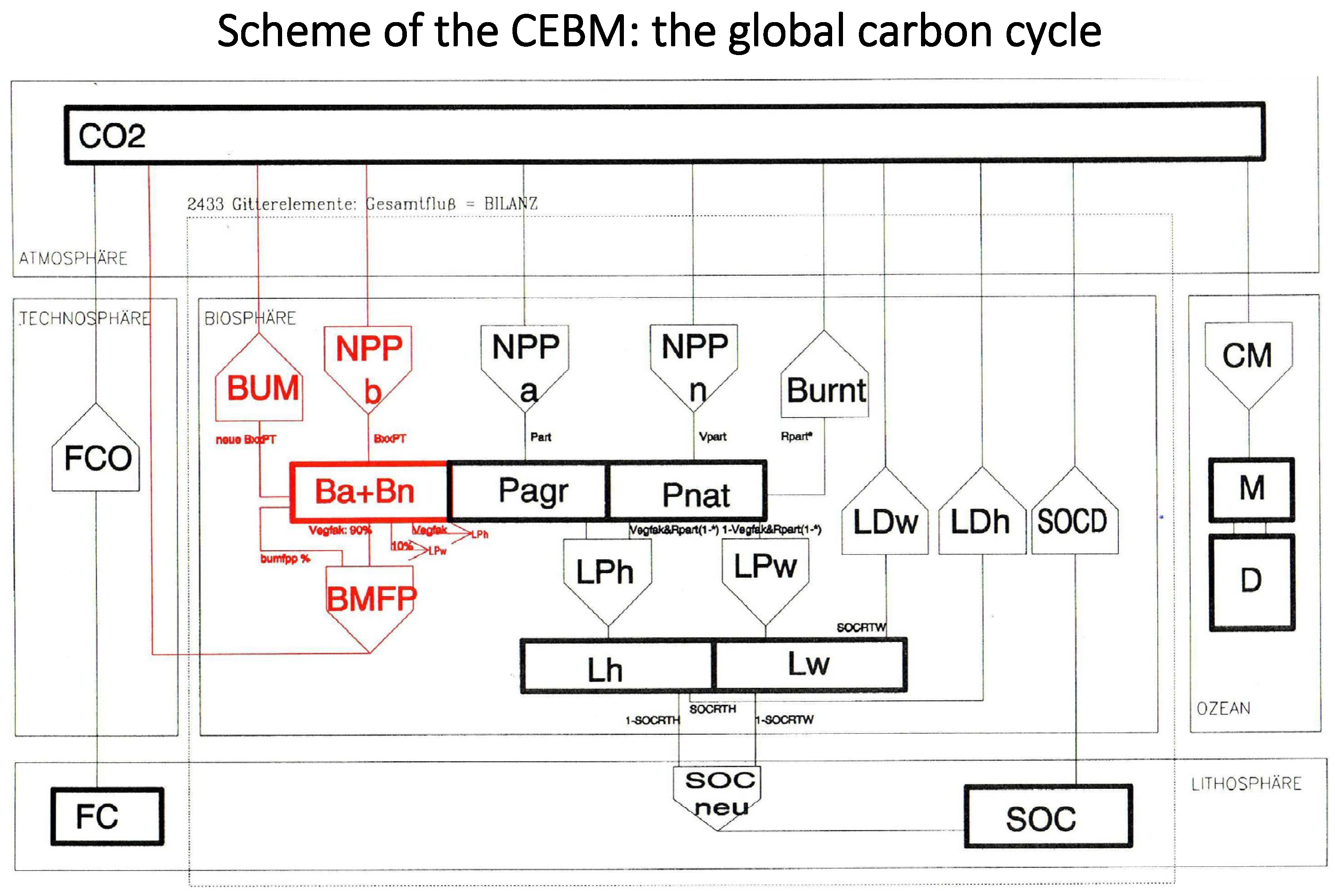
The next sections dwell on several model parameters which provide insight into the functioning of the CEBM and show their frequency distributions, geographic distributions and sensitivities. As mentioned later, the CEBM was constructed by the author by increasing the program volume of the initial program OBM to twice the initial length, mainly by adding the red components in Figure 15.

The essence of the CEBM is to model firstly the (undisturbed, i.e., natural) global carbon cycle) and secondly to model the alterations of this carbon cycle introduced by humans after extensive usage of biomass for energy on the entire globe. In order to be sure about the computational results from the CEBM, this article undertakes to visualise, study and reflect the most important changes with the global carbon cycles, starting from the undisturbed cycle and then including anthropogenic disturbances such as deforestation, fossil fuel use and usage of biomass energy for combustion that is grown in five different biomass energy strategies. While another article [44] reports in more detail on the computational results and interprets them in the light of literature, this article places the emphasis on analysing the usefulness of the model used.

This section explains what input and output parameter the used model has, what the spatial and temporal patterns of these parameters are and where the sensitivities of the models lie (Section 2.1). It shows what the author did to model the past few centuries in order to validate its correct behaviour under real, historic conditions, thus explaining the trust placed into the model for calculating future scenarios (model validation, Section 2.2). These sensitivity studies provide reasonable results which match with the actual historic development and thus allow to positively assess the reliability and validity of results in Section 3.

2.1. Representation of the Model Parameters

In the following section, the various CEBM model parameters are discussed in order to provide an insight into details of the data basis of the “Combined Energy and Biosphere Model”, the energy-related context of which was described recently as based on scenario techniques [77]. The biospheric part of the CEBM is based on detailed modelling while using the following biospheric data. Model input parameters (i.e., those shown until Section 2.1.3) exist as numbers for each of the 2433 grid cells. Almost all model output parameters (i.e., those pictured from Section 2.1.4 onwards) are represented as (a) grid-cell-dependent or (b) global totals of time series in the model. Several of these output parameters are shown in their context in the figure in Section 3.1, and listed in

Table 1. The list of CEBM model variables, issued yearly as a global sum. For their modelling context, see Figure 1 (at right) or (for a larger image) also Figure 15. Data source: as in Figure 2.

Variable	Unit	Designation
CO2	ppm vol	CO2 concentration in the atmosphere
FCO	Gt C	Fossil emissions accumulated over the years
PHYTE	Gt C	Global phytomass
NPP	Gt/a C	Global net primary productivity
LP	Gt/a C	Global inventory waste production (litter production)
LD	Gt/a C	Globally decomposed inventory waste (litter depletion)
M	Gt C	Accumulated increase in the oceanic mixed layer since 1860
D	Gt C	Accumulated increase in the oceanic depth layer since 1860
MD	Gt C	Accumulated increase in the total ocean since 1860
Pnat	Gt C	Global natural phytomass
Pagr	Gt C	Global agricultural phytomass
NPPnat	Gt/a C	Global production of natural phytomass
NPPagr	Gt/a C	Global production of agricultural phytomass
DPHYT	Gt/a C	Globally cleared phytomass
SOC	Gt C	Global reservoir of soil organic carbon at the beginning of the year
SOCD	Gt/a C	Globally depleted soil carbon
BURNT	Gt/a C	Global total of cleared biomass
Balance	Gt/a C	Global balance of the atmosphere ⟶ biosphere flow
FCO	Gt/a C	Annual fossil CO2 emissions
CO2Gt	Gt C	CO2 in the atmosphere in Gt

. For many of them, firstly maps or secondly time lines are provided in this article, in order to illustrate the functioning of the model, its geographical differentiation and its sensitivity of flows and pools.

2.1.1. Basic Climatic Data

The two most important driving climatic parameters in this biosphere model are the annual mean temperature and the annual mean precipitation. A map display with eight levels of grey shades and numerical values is shown in Figure 2 for these two input data sets. Figure 2 shows the global distribution of the annual average temperature as a map (at left) and as a frequency distribution (at right), for both temperature (a) and precipitation (b).

The frequency distribution for the global precipitation values shows an approximately logarithmic-normal distribution, while the frequency distribution for the global temperature averages shows a pronounced two-peak distribution (see frequency diagram inserts in Figure 2). Such a non-uniform distribution must be taken into account when choosing the intervals for sensitivity studies of both parameters.

According to ([80], p. 697), the “mean annual temperature and average annual precipitation data were derived from the WMO standard net of climate stations (data set from NCAR, Boulder, CO, USA), the World Atlas of Climate Diagrams [81], and a data collection with climatic zones maps by [82]. The data were interpolated and corrected for the mean elevation of the grid element”.

2.1.2. Basic Biological Data, Net Primary Productivity (NPP) and Phytomass (P)

The variable “soil” is used as a dimensionless multiplication factor to describe soil quality and can be found in grayscale representation in Figure 3 at left. A frequency distribution of these values, which vary from 0.4 to 1.7, can be found in the representation of the CO₂ fertilizer factor in Figure 3 at centre. The geographical distribution of this soil quality factor “soil” shows a very disparate picture. As expected, desert areas (e.g., Sahara and Central Asia) show low values for this multiplier for net primary productivity. A value of soil = 1 means that the theoretically calculated NPP according to the formula from Lieth and Aselmann [83,84] is used in the CEBM without correction. Values of soil > 1 mean that the NPP actually used in the model is greater than that of the stated theoretical formula of the preceding so-called Miami model (pictured in Figure 4). The variable soil is therefore dimensionless.

This “soil” data were generated according to ([80], p. 697) from the “Soil Map of the World” [85] as digitized onto the grid. Areas covered by the soil units were expressed as percentage of grid element area. 106 soil units were considered. Associated soils were excluded”. This is moreover documented as a table in ([80], p. 687).

There are several ways to visualize the formula for theoretical NPP (which in itself consists of various exponential term that do not lend themselves to immediate practical interpretation). Figure 4 shows from left to right NPP first as a function of temperature, then as a function of precipitation, then as a contour plot as a function of both (while offering the green dots for the distribution of “temperature-precipitation” data pairs and finally as a comparison with decomposition of herbaceous litter—to highlight the slightly different biological dynamics of growth and decomposition processes.

To describe the amount of matter in the standing natural plant cover (i.e., phytomass P, which represents a carbon pool), it is not exactly sufficient to use the annual net primary productivity NPP (i.e., the effective plant growth, which represents a carbon flux) according to the above-mentioned growth formula, but also the so-called stand age (Figure 5 at left) intervenes here (its source is described as a table in ([80], p. 690) and originates from [86]). Incidentally, an essentially multiplicative combination of both values forms the value for the phytomass, a graphical representation of which is given in Figure 3 at right. Depending on the vegetation zones, the variable stand age takes on larger values (e.g., tropical or boreal jungle) or is close to 1 (meaning years) when it comes to grasslands and steppes (Figure 5 at left). This term means the average age of the standing mature natural plant cover, which indicates the time period required for growth to reach a stable flow equilibrium in a specific vegetation zone. Since the stand age variable is reflected in the “existing plant mass” variable, the geographical distribution given here reflects the geographical distribution of the plant population (as density, Figure 5 at centre). As expected, the tropical rainforest areas as well as the temperate zones in Eurasia, the eastern USA and the Far East show a high stand age in the natural phytomass in the range of 100 years and above.

For reasons of comparison, the map of density of agricultural phytomass (based on per-country agricultural yield data, see [80]) is added in Figure 5 at right, with foci in industrialized areas and Southeast Asia.

2.1.3. Decomposition of Plant Matter (Litter Depletion LD and Soil Organic Carbon Depletion SOCD)

After growth of plants and standing plant matter, the next item in the natural carbon cycle (Figure 1 at right) is the decomposition of plant matter by microbial processes. The values for the annually degraded shares of herbaceous and woody litter are also shown graphically, as they again result from heuristic formulas deduced from global synoptics of measurements (Figure 6, in 3-dimenstional representation) (the formula genesis is described in ([80], pp. 692–693) and originates from [87,88]). Figure 7 provides the 2-dimenstional representation regional distribution and comparison by regression with other parameters. As mentioned, both Figures show the two- or three-dimensional representations of the degraded proportions as a function of temperature and precipitation because these heuristic functions have a key role in controlling the global carbon cycle.

Furthermore, the biological type of standing vegetation is determined in the CEBM by the “vegetation factor” which indicates the proportion of herbaceous plant mass in the total plant mass (its source is described as a table in ([80], p. 690), rightmost column] and originates from [86]). It varies from about 30 to 100%, as can be seen from the map illustration in Figure 8 at left. This value will be relevant for the biomass fuel scenarios because the woody but not the herbaceous component is used for combustion in several scenario types. Areas with a high herbaceous content coincide with the well-known desert areas of the world: Sahara, Arabia, Central Asia and central Australia, southwest Africa, the Midwest of the USA and finally the coldest continental areas of the world in the north. If you read this figure the other way around, i.e., looking for areas with a high proportion of wood in the plant mass, you will see mainly the three tropical areas (South America, Central Africa and Indonesia) as well as the temperate belt of the northern hemisphere.

Furthermore, the division between naturally vegetated and agriculturally used areas is of great importance: The variable shown in in Figure 8 at centre indicates the proportion of agricultural area in the total area of the respective grid element, which adds up to 100% with the natural area share. From this map it can be seen that these areas largely correspond to the settlement zones of humanity. For the sake of completeness, it should be noted that areas used for meadows or pastures also fall into the category of agriculturally used areas; this area share lies between 60 and 100%, particularly in some areas of Europe, Ukraine and to the east, in Eastern China, India and the American Midwest. As a mirrored image of the proportion of agricultural areas, Figure 8 at right shows the proportion of naturally vegetated areas in each grid element: in the overwhelming majority of grid elements this is more than 99%.

Finally, agricultural productivity, which differs from natural productivity, is indicated by a separate input variable, which is assumed to be almost evenly distributed within a country (Figure 9 at left). By the way, in grid elements where the agricultural area share (Figure 8 at centre) is zero, the value for agricultural productivity (Figure 9 at left) is also allowed to be zero. Figure 9 at centre and at right offers a possibility to compare the geographic pattern of agricultural productivity with the geographic pattern of natural productivity (while these use slightly different units for their map representation).

With the help of an additionally entered variable for the geometric (i.e., geodetic) area of a grid element on the earth surface and the variable of agricultural productivity, it can be computed that globally around 16.3% of the continental area (excluding Antarctica) is used for agriculture.

2.1.4. Political and Economic Input Data

The structure of the program architecture in the CEBM determines that each grid element corresponds is assigned to one of 119 states. On the computational level, it cannot be the case that a grid element belongs partly to one state and partly to a neighbouring state. Although this predetermined program structure may be detrimental to data accuracy in very small countries, it does not noticeably affect the global final result due to the large number of grid elements.

The country classification mentioned is used for the entire energy strategy program module and will be important there. As mentioned, the coarse grid can lead to data inaccuracies in small states because the exact geodetic localization of the state borders does not correspond to the borders of the grid elements. Sometimes a grid element contains several countries (e.g., the Benelux countries, containing Belgium, The Netherlands and Luxemburg). The grid element for Austria is located northeast of Vienna. As an example, the width of the Alps is only two squares, which leads to climatic uncertainty. If one wishes to use biospheric data for individual small countries, it is important to take into account that the numerical values must be adjusted, at least because of the artificial geometric rectangle area, which is different from the actual country area. Likewise, most accurate databases on deforestation, economy and energy supply are broken down by country.

2.1.5. Historic CO₂ Emission Data

The global sum of energy-related fossil CO₂ emissions from 1860 to 1988 is given based on the very useful available source [89] and subsequent updates, which includes a country-by-country breakdown of carbon emissions annually since 1950 and was published at Oak Ridge National Laboratory (ORNL). This data, differentiated by energy source, almost seamlessly continues the data that has already been available in the CEBM since 1860 into the recent past [90]. The only carbon-containing energy source not taken into account in this data source, but very important, is the energetic use of biomass that has been ongoing since the beginning of human civilization, which is referred to as “traditional biomass” in CEBM’s energy scenarios ([91], pp. 59–64).

2.1.6. Input Data for the Energy Strategy Module: Population and Economic Growth

Energy scenarios were described in much detail elsewhere ([91], pp. 301–310; [44,92,93,94]). For the detailed energy scenarios for the CEBM, a completely new program module was created. The data required for energy economics is not broken down into grid elements (as the biospheric data) but rather into countries because these form meaningful energy economic units given the same energy policies applied. However, it would still be possible to transfer this country-wise data to the level of grid elements with the help of a database created by the author containing the population distribution of the earth. For this purpose, the population density from an atlas was entered for each grid element [95], which was used as the best after having compared three atlases.

The result of this process, namely the global distribution of population density, can be seen in Figure 10 at left. With the help of this population database, it is now possible to distribute country-by-country data (e.g., emissions) approximately accurately (but sufficiently accurate, for the global model’s targets) across the area within a state according to the population distribution (for results see, for example, ([90], pp. 60–64)). In addition, the information for the annual rate of population increase in the individual countries (which is assumed to decrease by 1.6% annually to provide results consistent with the UN estimate; ([78,90], p. 113), taken from the same data source is shown in ([78,96], p. A11/3) and in in Figure 10 at centre while the scenario for the 2100 population distribution is shown in Figure 10 at right—showing a massive shift of earlier centres of gravity.

The connected estimation of GDP growth includes saturation effects within the richest nations ([78], p. 118) which conforms to both experience and the sustainability paradigm of saturating material turnover. Resulting economic levels (measures as GDP/capita) are pictured in Figure 11 at left, and resulting geographic patters of GDP per grid cell in Figure 11 at right. Energy scenarios resulting from these socio-economic patters are discussed in detail in [97,98,99,100].

In order to provide an overview of the main model parameters, Table 1 lists the key global parameters, of which many are pictured in this article as a timeline.

2.2. Checking Accuracy and Sensitivities of Various CEBM Program Parts

In the following section, the various CEBM model parameters are discussed in order to provide an insight into details of the data basis of the “Combined Energy and Biosphere Model” (compare the list in Table 1). For a quick start, it was doublechecked whether the historic (and thus experimental) data path of atmospheric CO₂ concentration values was correctly modelled (“ex post”) by the CEBM, which could be clearly answered by “yes” (thus, no figure, see ([78], p. JB91-6). Furthermore, early enough the plausibility of the dynamics, elasticity and resilience of the ocean subroutine was assessed ([78], p. A5-1-5), a user-friendly macro for creating geographic maps was created by the author ([78], p. A6-1-8), the plausibility of the used country-wise emissions data was doublechecked ([78], p. A7-1-5), and the arithmetic appropriateness of the biological formulas governing the carbon cycle was evaluated through graphic representation ([78], p. A8-1-18).

2.2.1. Sensitivity Studies through Preparatory “Zero Runs”

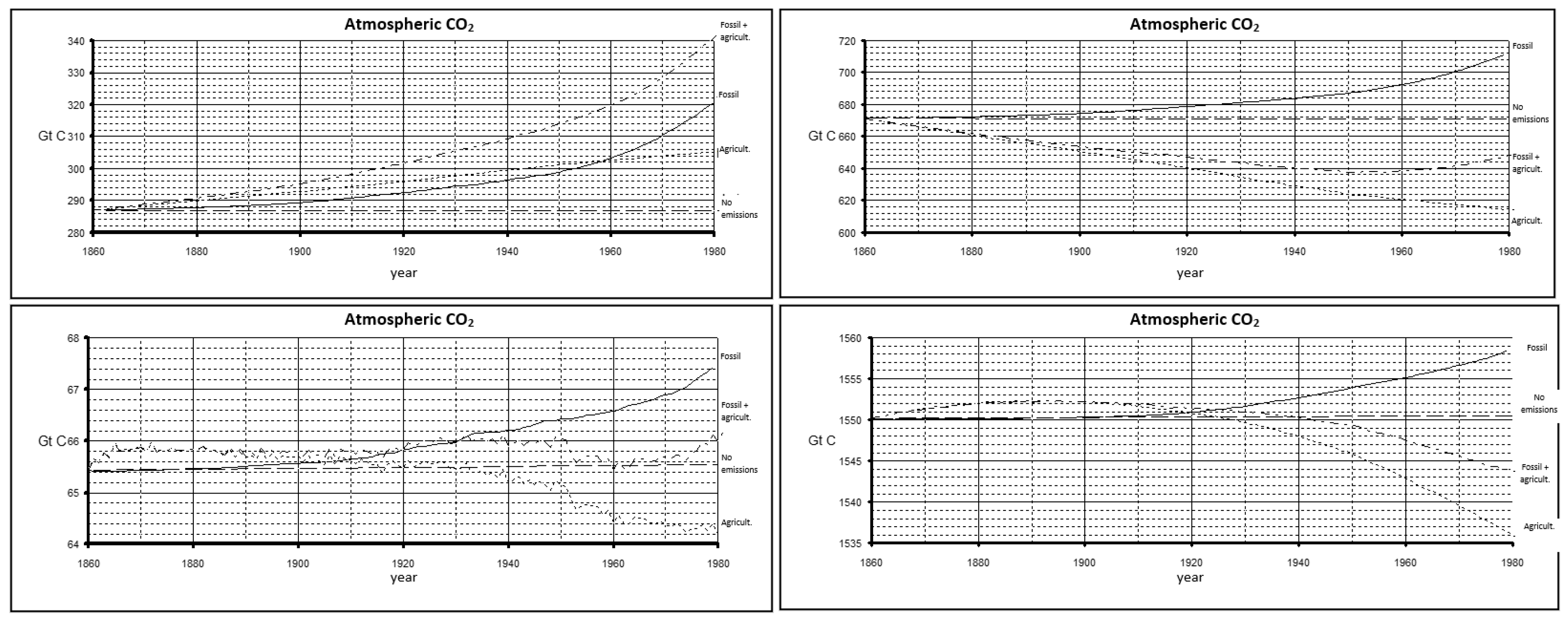
In order to demonstrate the computational efficiency of the CEBM as a hypothetical historic study, fossil emissions or emissions due to land use changes or both were set to zero (these start in 1860). The latter calculation variant (i.e., without any anthropogenic CO₂ emissions) actually showed a constant atmospheric CO₂ content (meaning that the CEBM program did reach the required state of equilibrium within the natural annual carbon cycle). The other two mentioned test runs make it possible to dissect the influence of fossil emissions and deforestation emissions on the historical increase in CO₂ into two separate effects. It turns out that until 1900, agricultural emissions mainly contributed to atmospheric CO₂ (Figure 12 above left). Around 1950, both sources contributed equally, and later fossil emissions contributed significantly more to the rise of atmospheric CO₂ concentration levels. Similar signals within a hypothetical (i.e., only partially disturbed—as a historic what-if analysis) carbon cycle emerge in the global pools of phytomass (above right in Figure 12) and in litter as well as organic soil carbon (below in Figure 12).

Moreover, Figure 12 above right shows that the fossil emissions seem to have resulted in a fertilization effect that increased the stock of global phytomass in the model by over ten percent (in case the used formulaic representation of the fertilizer effect is that exact). However, through deforestation, this phytomass was decimated by more than this same amount. The timeline of the variable litter, on the other hand, is more complicated: until 1900, the clearing contributed to a slight increase (biomass remaining on the ground after the clearing process), from 1900 onwards this compartment decreased compared to the standard run because of the lower phytomass in absolute terms (Figure 12 at below left). The same applies to organic soil carbon SOC (Figure 12 below right).

This modeling of an “imaginary history” in which only one of the two main CO₂ emission sources would have existed can serve to better understand the effect of future human interventions in nature.

2.2.2. Sensitivity Studies as a Result of Different Deforestation Scenarios

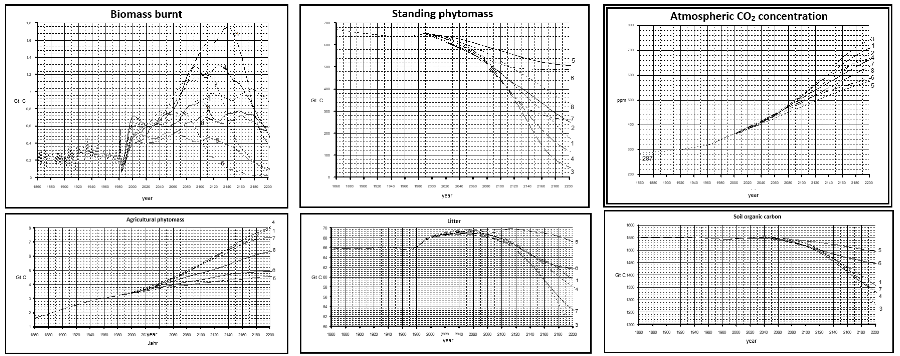
One of the key sensitivities of the modelled global carbon cycle is certainly its response to diverse deforestation scenarios. These can differ quite widely theoretically (i.e., just for arithmetic reasons, not to illustrate realistic practicability), namely ranging from maintaining the current plant cover to complete elimination by reckless total deforestation of the entire planet.

Figure 13 shows the eight different deforestation scenarios which are based on the principal understanding that deforestation activities in a grid cell are influenced by previously occurring deforestation activities in neighbouring grid cells, but with variable probabilities of geospatial propagation. The amount of biomass burnt immediately in a given year (at left in Figure 13) results in an even larger amount of biomass that decomposes according to the existing formulas for plant decomposition, thus picturing the longer-term effects of destruction of a forest. Figure 13 at centre shows the standing plant matter which in the year 2100 varies from ten to eighty percent of the existing amount, while scenario number 5 is the most optimistic scenario (in the sense of preserving forests) and scenario number 3 the most pessimistic one. Figure 13 at right shows the resulting atmospheric CO₂ concentration until 2100 which interestingly does vary but not enormously, when comparing to the variations caused by scenarios with diverging fossil emissions ([91], p. 307).

2.2.3. Assumption of a Uniform Atmosphere

Since the global earth’s atmosphere mixes within 1 to 2 years [101], the assumption of a single numerical value for the CO₂ content in the entire earth’s atmosphere is justified for the calculation accuracy required here. The seasonal fluctuation in CO₂ content detected by measurements due to the growth and decay of plants in the annual cycle (including the iconic and historic Mauna Loa experiment curve) is not taken into account in this model on a monthly basis, but this does not affect its suitability for solving long-term energy management issues. Likewise, a CO₂ concentration gradient from the northern hemisphere to the southern hemisphere can be verified experimentally (e.g., [62]). However, the resulting concentration difference between north and south is very small compared to the increase in concentration over several decades. For this reason, it is also justified that the regional distribution of energy-related CO₂ emissions on the one hand and CO₂ absorption by the oceans on the other hand is not modelled at the grid element level in the CEBM.

2.2.4. The Biospheric Carbon Fluxes

The degree of validity or accuracy of the formulaic relationships in the CEBM will now be examined.

With regard to the formulas for growth and degradation of plant matter, it can be seen as confirmation of the accuracy of the CEBM that a value of around 660 Gt C for the “phytomass” reservoir occurs in the steady state during the preliminary run, as is compatible with literature ([77,84,88], p. 5). The same applies to the litter pool (approx. 70 Gt C) and the soil organic carbon pool (approx. 1550 Gt C) reservoirs. An advantage of the CEBM as compared to other models discussed earlier ([88], p. 3) is the distinction between herbaceous and woody biomass. A graphical representation of the comparison of the two degradation constants with one another or the shares of biomass degraded with one another can be found in Figure 7 (2nd and 4th from left). This shows that as a rule of thumb, herbaceous biomass is decomposed about 2.5 times more (or faster) than woody biomass. Of course, the rate of degradation is also correlated to a certain extent with the net primary productivity of the natural vegetation, which is shown in the rightmost image in Figure 6.

On the other hand, the mathematical representation of soil carbon degradation in the model suggests that exact information for such complex processes is difficult to find: the degradation rate for soil organic carbon is one hundredth of the degradation rate for herbaceous stand waste (Figure 7 at right). The resulting flows for the degradation of soil carbon correspond to the expectations of experts in ecosystem research ([79,83,84,88,102]), but may represent only one of several possible attempts at quantitative description. In this context, attention should be paid to the complex processes involved in mineralization (degradation of organic material through microbes) in the different soil layers. The extent of this degradation depends on many local factors that are difficult to describe in a global model in their local details.

2.2.5. The Ocean Model

Since the thematic core of the model is in the area of biospheric cycles and not in the area of oceanic carbon cycles, a simplified model was used to model the CO₂ absorption processes in the global ocean. The physical process of the diffusion of CO₂ into the several assumed deep layers of the ocean is modelled in a dedicated sub-program. However, other approaches to modelling processes in the ocean can also be found in the literature, which are listed below according to the degree of spatial differentiation:

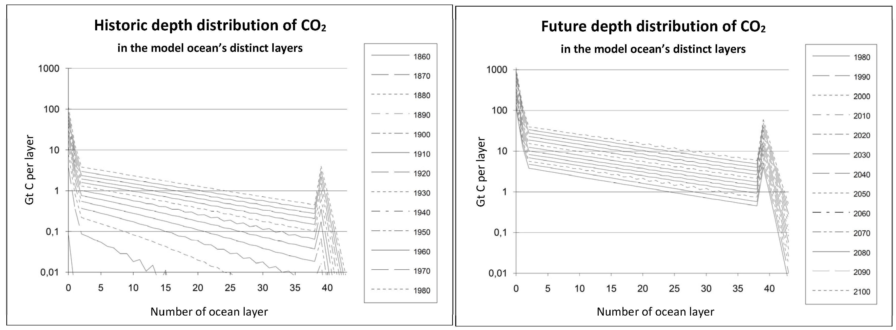
• The model used in the CEBM is a one-dimensional “box-diffusion model” with spatial resolution only in the vertical axis, but not along the earth’s surface (see Figure 14 at left and second left).
• A first improvement would be the differentiation into different latitudes (two-dimensional models). Here the global ocean is divided into ring-shaped zones surrounding the globe. CO₂ diffusion also occurs between the various ocean rings. Each of these sub-oceans is assigned the corresponding geographical extent, which comes from the distribution of the continents on the globe.
• Two-dimensional “upwelling” models: In addition to diffusion, vertical mechanical mixing of the ocean’s water masses is assumed. This also means that carbon is transported in the form of CO₂. An example of this is the model designed [103] at IIASA. This also has a “wind-driven” component, which models the movement of oceanic water masses due to wind activity. The flow conditions are shown in Figure 14 at third left, where only the northern hemisphere is taken into account.
• Three-dimensional ocean models with spatial resolution in all three coordinate directions are being developed, for example, at the Max Planck Institute in Hamburg (MPI) for Meteorology. Horizontal flows circulating around the globe can also be depicted (see Figure 14 at fourth left). Such models are connected to the “High Resolution Biosphere Model” (HRBM) by [104] as part of the European carbon cycle modelling program ESCOBA [103,105,106,107]. The reference value of 1.8 Gt C can serve as a guideline for the absorption capacity of the model ocean of the Max Planck Institute (MPI) Hamburg according to an oral communication by authors Heimann and Meier-Reimer at MPI. This value is slightly lower than the value of the model ocean used in the CEBM, and thus seems consistent.

After reflection of the advantages and disadvantages of the several available ocean models, the author concluded that the already included ocean model is sufficient for the envisaged task, namely to compute the net effect of large-scale energetic biomass use. Other modelts might be more exact regarding geographic distribution across the planet’s oceans and regarding vertical mixing processes, but these details do not visibly influence the final result of the CEBM major task, namely to yield the net increase in atmospheric CO₂ concentration after a period of a few decades. Therefore, the decision was made to leave the initial ocean submodel as it is. This decision was corroborated after several long discussions with expert modellers at the International Institute for Applied Systems Analysis (where the author was affiliated for several years) and at the Hamburg-based Max-Planck Institute for Meteorology (in the frame of semi-annual C cycle conferences) who undertook the ocean modelling for many current C cycle models.

As a principle, different chemical reactions have different characteristic reaction times. As an examle, CO₂ can be absorbed by the atmosphere within a few years while the complete resorption of elevated atmospheric CO₂ concentration my take much longer because the diffusion of CO₂ through the oceanic deep layers proceeds only very slowly. The second-right image in Figure 14 shows how long it takes for a (fictive) CO₂ pulse to be buffered by the global ocean (equivalent to a fictive +5%/a growth in fossil CO₂ emissions—which by the way leads even to an early exhaustion of fossil reserves).

In the view of this image (and its stacked equivalent in the rightmost position of Figure 14) it becomes plausible to speak about a century for the buffering effect time constant of the ocean. In other words: for the deep ocean, not only the present-day CO₂ concentration value is relevant but also the values of the past decades to century. This means: the global carbon system and especially the ocean has a “memory”.

The operation of the ocean subprogram is crucial to the final result because the ocean is the main recipient of CO₂ in the global cycle over long periods of time, such as a century. This can be clearly seen from Figure 14 overall.

3. Generating Results

3.1. Modeling Biomass Fuels

One of the two main features of the CEBM (as different from usual biosphere models) is the inclusion of the possibility of using biomass for energy. To achieve this, the equations for carbon flows in the biosphere had to be changed in order to be able to model the growth and extraction of biomass fuels. These fuels are then to replace fossil fuels, taking into account the different calorific value (but not the different efficiency of technological combustion).

The model consideration of the energetic use of biomass should, on the one hand, do justice to realistic processes, but on the other hand should also correspond to the unavoidable prerequisite for sustainable biomass use. This required sustainability means that natural resources are used in such a way that subsequent generations have the same options for use (e.g., [62]). For the special case of using biomass for energy, this means in particular that the existing plant mass should not be reduced during cultivation, but only the annual increase is used to generate energy. A definition of further criteria for sustainability can be found in [108], which also contains a definition of sustainability using a system-dynamics way of thinking.

This prerequisite for sustainability, which has been unwaveringly specified from the beginning of the modelling work, is represented in the CEBM as follows: The flow leaving the “phytomass” reservoir is called litter production (see at right in Figure 1, or in Figure 15, with the biomass-fuels-related additions in red). As already mentioned above, its size in stable equilibrium is identical to the net primary productivity. Regardless of whether the biomass fuels are harvested annually or at longer intervals, the long-term average of the biomass removed must be the same as that amount which grows annually, as is the case in classic forestry, for example. The flow “litter production” is now redirected: it no longer flows into the litter compartment, but forms the flow “biomass fuel production” (BMFP). The plant material is taken from the ecosystem via this flow and is to be used as fuel by the energy industry. In order to model the conditions as realistically as possible, it was assumed that 90% of the woody plant material, but not the herbaceous plant material, are used as fuel. The remaining material flows into the inventory waste as usual. In short, the energy industry harvests the wood that grows annually on the various areas in order to use it for combustion.

In this paragraph, an unexpected modelling result is described that might be difficult to understand at first sight. As was already shown in the first test runs after implementation of the energetic usage of biomass, somewhat unexpectedly, the following quite specific amount of plant carbon represents a significant amount that must be closely monitored in order not to violate the balance equations: it is the large amount of plant material that grows on an area before this area is used (or “dedicated”) for energy production. For example, if plantations are created on formerly primordial forest areas, the volume of the primordial forest biomass must be dealt with—and this is quite huge. This amount of carbon is labelled in the CEBM as “BUM” (standing biomass on the re-dedicated areas, “Biomasse-Umwidmung” in German language) in the flow chart in Figure 15. Of course, it would be unwise to intentionally erect plantations on the location of densely grown forest area, but recent history showed that exactly this actually happened, most deplorably [109,110]. In terms of program technology, it was planned that these quantities of plant material could either be partially or completely utilized for energy purposes (i.e., burnt in a combustion facility) or could be emitted directly into the atmosphere (i.e., burnt in the sense of blunt deforestation by fire). The control variable for steering the carbon flow “BUM” is called “bumfpp”, as is also mentioned in Chapter 3.2.1 of the [111] annual report. In practice, a biomass energy industry should of course try to avoid these undesirable emissions as much as possible—but did not at all, as practice showed.

The exact results of this part of the program can be found in [44,64] and in the following sections.

3.2. Modeling the Processes Associated with Deforestation

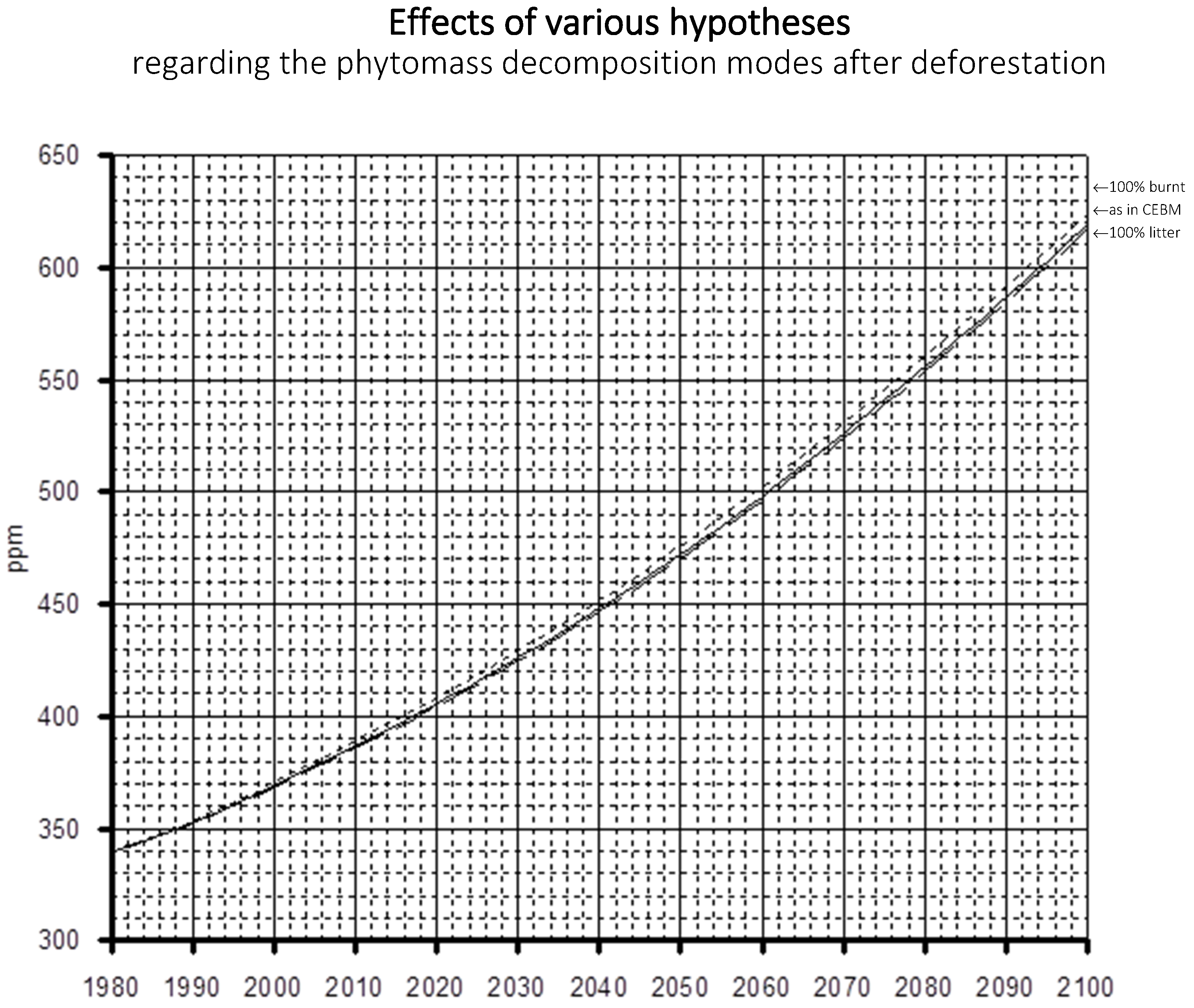
The influence of the deforestation processes themselves on the CO₂ concentration has already been mentioned in more detail previously (see Chapter 3.1.2 in the 1991 annual report at [111], and in [64]). In the present section it remains to be described how big the impact on the atmospheric CO₂ concentration will be under the CEBM’s assumption that 50% of the herbaceous and 30% of the woody cleared plant material is immediately burnt and emitted. For this purpose, two test runs were carried out with the following extreme assumptions, each of which were opposite: one time, the entire (herbaceous and woody) plant mass should be emitted immediately, another time, nothing at all should be emitted immediately, but 100% should follow the usual degradation path via litter and soil carbon. Figure 16 shows that such model variations (i.e., assumptions regarding the exact procedures after deforestation) ultimately have a very small influence on the final result of the atmospheric CO₂ concentration.

3.3. Where Does Emitted CO₂ Ultimately Go?

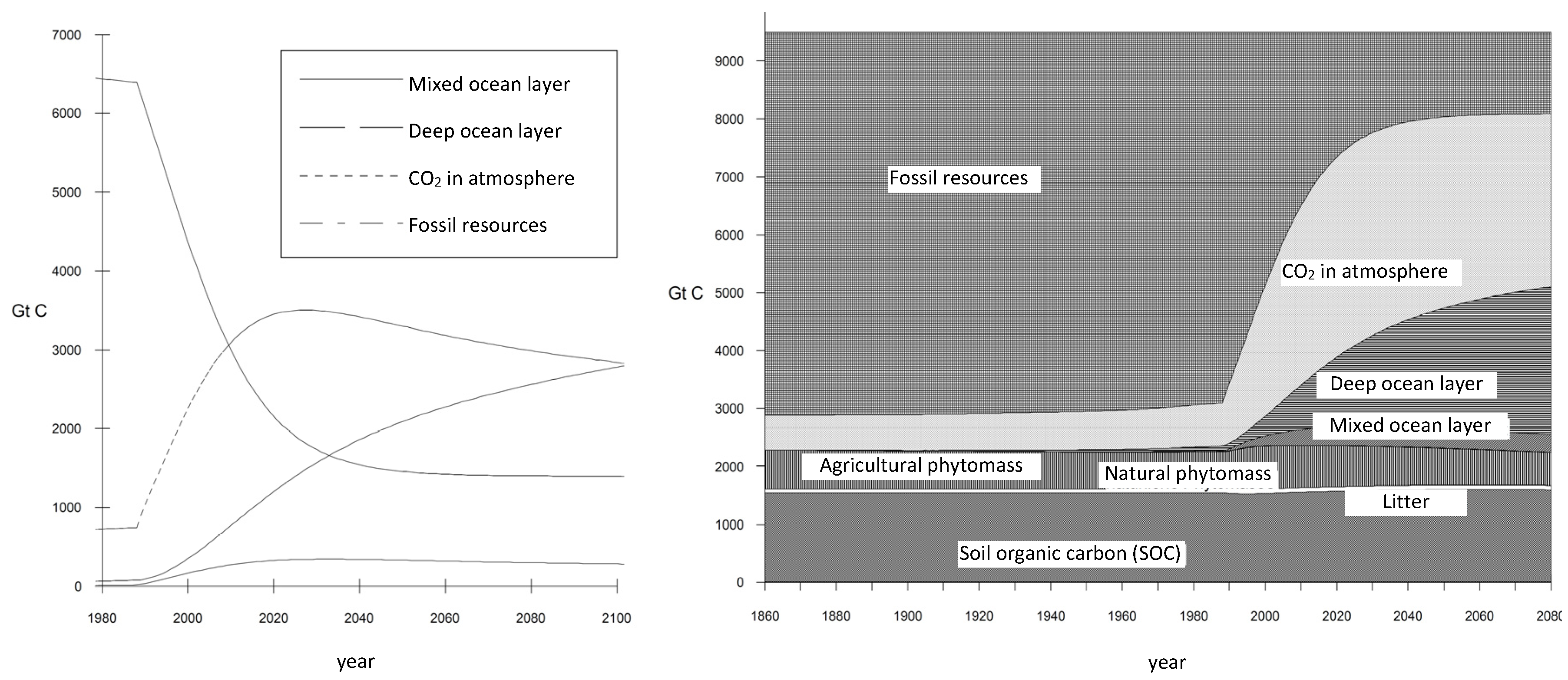
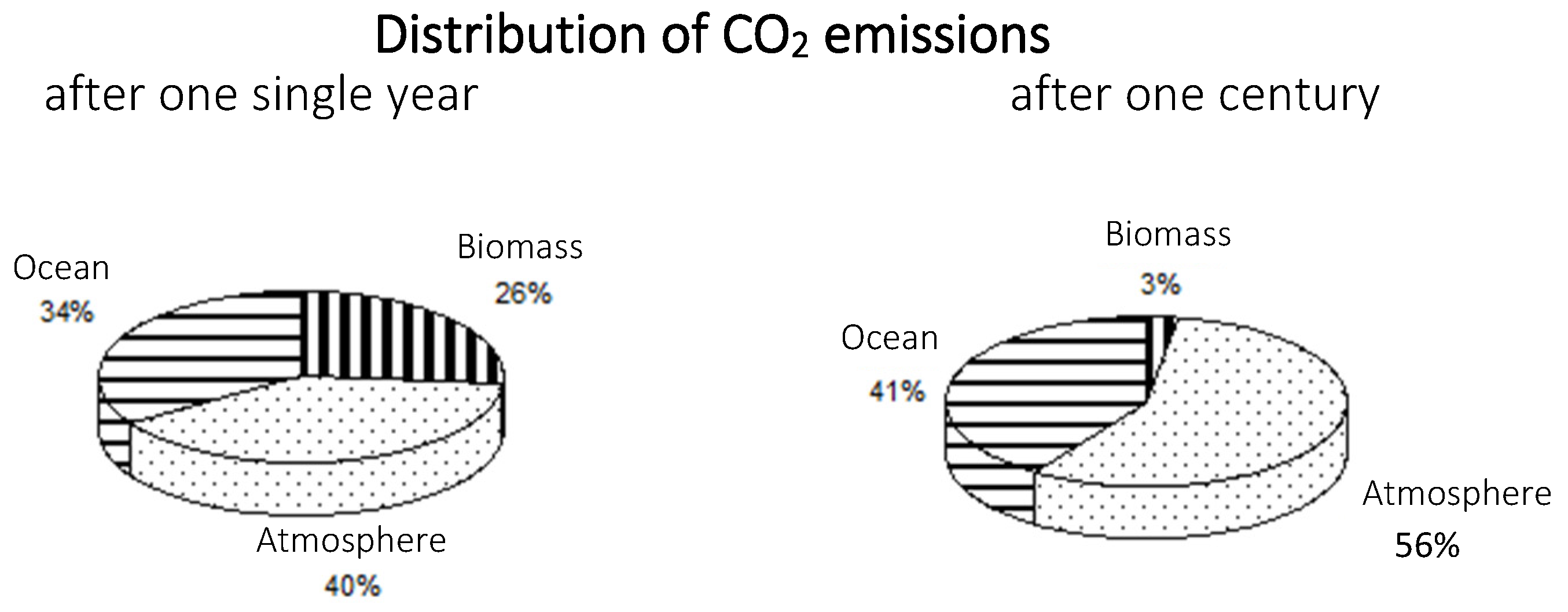
For an initial rough estimate of the complex dynamics and time behaviour of the global carbon cycle system, one can consider in which compartment the emitted amounts of CO₂ will be ultimately deposited. The pie charts of Figure 17 and also Figure 14 at right provide information about this question: When considering one single given year (Figure 17 at left), CO₂ emitted from fossil or deforestation sources remains (i) in the atmosphere and in almost equal proportions (depending on the reference period considered) it is absorbed (ii) by the ocean through the mechanism of diffusion and (iii) in the biomass through the mechanism of the fertilizer effect. However, when considering a century, a more precise specification of the various carbon repositories is possible, but difficult because of the Earth’s constantly flowing carbon streams. In this sense, Figure 17 (at right) quantifies that slightly more than half of the emitted carbon dioxide geos into the atmosphere while almost the other half goes into the ocean—a long-term distribution well in line with Figure 14 at right.

In a given single year (Figure 17 at left), the CO₂ absorption into the plant cover through the fertilization effect is counteracted by global deforestation activity. The clearing processes, in turn, comprises firstly a spontaneous emission pulse due to combustion and secondly a flat emission process lasting several decades due to the rotting of dead plant matter. The ocean, for its part, has a CO₂ absorption characteristic that absorbs a CO₂ pulse (that suddenly occurs in the atmosphere, just to show the effects by this hypothesis) only over several decades. For all of these reasons, as well as because of the different time constants of the individual carbon fluxes in the biosphere, it is difficult to accurately identify (diagnostically) the emissions of a single year as an increase in the various carbon reservoirs. That’s why the two diagrams in Figure 17 at left and at right differ so considerably from each other. Rather, the global carbon cycle represents a dynamic system that is constantly in flux—and this is an important structural message understood when contemplating the various CEBM model runs presented to date.

3.4. Results Regarding Carbon Neutrality of Biomass Fuels

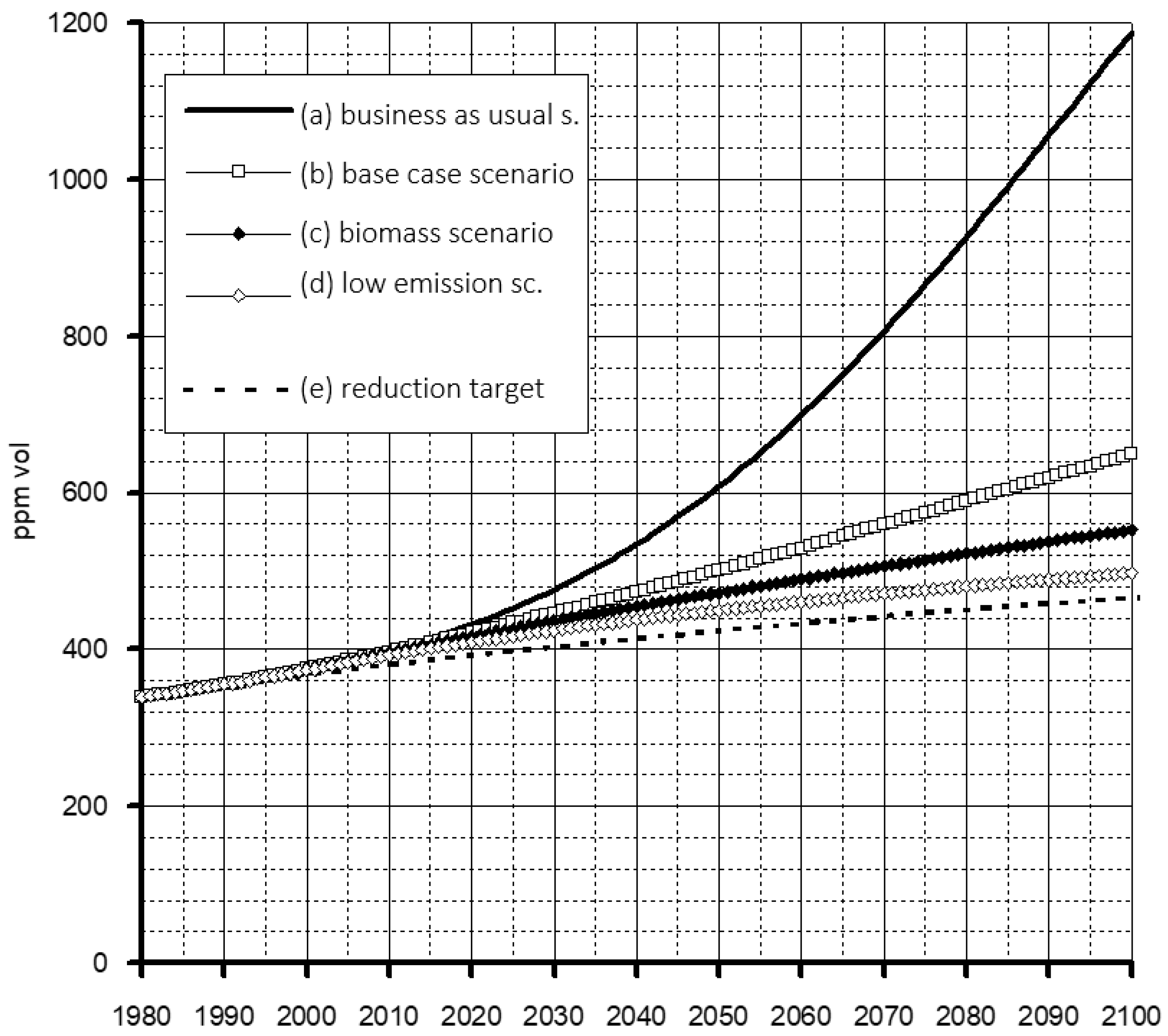
After the preceding sensitivity studies that served to analyse the behaviour of the CEBM when selecting diverse input parameter, one important set of scenarios [44,46,47] is undertaken which picture (i) energy usage from biomass versus (ii) energy usage from completely carbon-free energy sources such as solar and wind. Figure 18 displays (a) the business-as-usual scenario (at the top) and (b) the base-case scenario (second from above—and the message of this comparison a-b is that diminishing the annual growth rate of energy demand will decisively lower atmospheric CO₂ concentration. Furthermore, starting out from the mentioned base-case scenario’s energy demand, the (c) biomass scenario uses almost the maximum of the world’s theoretical potential for biomass energy growth—covering gradually all available areas until the year 2100 by energy crops or energy forest. Next, (d) the low emission scenario assumes the same annual global energy demand as the two preceding ones but covers it with truly carbon-neutral energies such as solar and wind. And, still below (e) a global reduction target is visible. Overall, the comparison of lines c and d signifies that biomass strategies lower the atmospheric CO₂ concentration only halfway but not fully [44,64]. Hence, biomass fuels can be seen as “half as carbon neutral” as widely assumed on a quick theoretical level.

The train of thought when interpreting scenarios (a) to (d) in Figure 18 is as follows:

(a)

The business-as-usual scenario represents to point of start for all scenario thinking (i.e., what-if logic) and means the threatening but likely future status which should not at all take place because of its clearly climate-threatening effects.

(b)

The base-case scenario means an already (over-)optimistic future for which enormous reductions in energy demand growth must be achieved, namely lowering the annual growth rate from +3% to +1%.

(c)

The biomass scenario means to start out from the energy demand defined by the (optimistic) base-case scenario and to cover it by biomass fuels to the extent which was computed by the CEBM as the planetary maximum.

(d)

The low-emission scenario means the same as above only that all biomass in (c) is replaced by non-carbon energy in (d). Consequently, any difference between the (c) and (d) scenarios equals the amount to which biomass fuels are not truly carbon neutral.

(e)

As an orientation, this scenario means a current reduction target. It is this emission path that actually should be reached for a sustainable and climate-compatible future.

3.5. On the Degree of C-Neutrality of Biomass

The above result can be explained as follows: According to the results of the CEBM, the removal of plant material from an ecological system over decades will deplete the (litter pool and more strikingly, because of its long-term nature) the pool of carbon in the soil (Figure 15, item SOC). This depletion of soil organic carbon becomes noticeable after decades and represents net carbon dioxide being emitted ultimately into the planetary atmosphere, just as did CO₂ after forest clearing, forest burning and subsequent long-term degradation of stems, twigs and leaves in a deforested forest: these emissions will be dispersed in the planetary atmosphere and ultimately half of it into the ocean (as already was shown in Figure 17 at right). Looking quantitatively at these systemic net CO₂ emissions (emerging from the organic soil layers) shows that approximately half of the initially avoided (fossil, energy-related) emissions emerge as biosphere-related emission—as a result of the interlinked carbon fluxed. Therefore, systematically, the cultivation and extraction of bioenergy engenders half of the avoided emissions through the “back door” of soil depletion [25].

On the level of envisaged carbon compartments, the soil carbon quantitatively stems from the activity of microbes that (as usual) decomposed dead plant matter. The flux from the SOC reservoir (namely SOCD, see Figure 15, modelled according to the formulae visualized in Figure 7) stays identical as before biofuel extraction (because microbes “do not know” whether new litter, LD, is flowing into the compartment SOC or not). Consequently, SOC decreases by the amount that corresponds to this same litter which is no more produced after large-scale extraction of biofuels from those areas. Thus, C can no longer, as was usual under natural circumstances, flow along the path “litter ⟶ SOC” (see Figure 15).

Therefore, any strategy of planet-wide biofuel production, extraction, and usage means a vast redirection of planet-wide carbon fluxes. Furthermore, such human action distorts an existing dynamic equilibrium of stable flows and counterflows, namely the natural carbon planetary carbon cycle. These fluxes of C are instead used by humans to generate energy by combustion and are (as the model results tell) therefore no more disposable for sufficient humus formation by natural procedures in the pertinent soil layers.

It may admittedly be that the CEBM’s modelling results are not exactly accurate in terms of numbers, but given the current knowledge of the C cycle, it remains true undisputedly that an impoverishment within the soil compartment actually takes place. The extent of this depletion is most likely remarkable and meaningful in the long term, even if it may depend on the locally prevailing structure of soil horizons.

It can be recalled here that the approach of scenario-writing for the CEBM was to assume an (even thoroughly unrealistic) maximum worldwide usage of annually grown woody plant matter for its direct combustion, regardless of its practical feasibility and ethical appropriateness. Under the impression of the above-mentioned effects of biospheric CO₂ net emissions and soil depletion, one might wish to resort to just diminishing the amount of area dedicated for growing biomass for combustion, and to undertake modified strategies on a smaller scale. Although such scenarios have much less impact on the Earth’s ecosystem, they (quite expectably) then offer only a minimal desired effect to curbing the greenhouse effect [44].

3.6. Comparison of the Mitigation Potential of the Different Scenarios

As far as the net mitigation of the greenhouse effect, i.e., the carbon dioxide concentration in the atmosphere (see Figure 18) in the various scenarios is concerned, we see that moving from the baseline to the biomass timeline equates a reduction of CO₂ emissions by only 0.5%, as summarized in

Table 2. Comparison of the size of the CO₂ reduction that can be achieved by the year 2100, according to the CEBM calculations, as described by the model runs in Figure 18.

Scenario	Atmospheric CO2 Content in the Year 2100	CO2 Reduction Compared to the Trend Case for 2100
Trend = business as usual (+3%/a increase in emissions due to the increase in energy demand)	approx. 1200	-
global maximum biomass use (in trend scenario: +3%/a)	approx. 1000	approx. −150
Reducing the increase in emissions or energy demand from +3% to +1% (base scenario)	approx. 650	approx. −550
Combination of both methods (biomass scenario)	approx. 550	approx. −650
Reduction target (−1%/a)	approx. 450	approx. −750

. In 2100, the atmospheric CO₂ saving due to switching from the trend to the base scenario (i.e., energy consumption is reduced by two percentage points) amounts to some −550 ppm (Figure 18). The achievement through the theoretical maximum of universal energy use of biomass amounts to (only) −150 ppm (Figure 18). As a comparison, when viewing a climate-friendly path, a reduction of around −740 ppm is required. Thus, any prioritization of measures against the greenhouse effect must be carried out with the strikingly different magnitudes above.

To put it clearly, global maximal energy use of biofuels only produces 100 ppm. Thus, a global reduction in energy demand in inevitable.

This result of the model, namely that the priority is to reduce the rate of increase in energy consumption, is also in agreement with a large part of the literature such as [112,113,114,115,116,117,118,119,120,121,122,123,124,125,126,127,128,129,130,131,132,133,134,135,136,137,138,139,140,141,142,143,144,145,146,147,148,149,150,151,152,153,154,155,156,157,158,159,160,161], as thoroughly discussed in ([44], pp. 21–25).

4. Conclusions

The intention of this study was also to provide a decision-making aid for energy planning on the socio-political and practical levels. For this reason, the following will be used to derive from the results of the work how the energy policy of an industrialized country should act. As an application example, we could see how the earlier energy policy of an industrialized country (such as Austria) met its existing goals of meeting demand (demand reduction), economic efficiency (security of supply), environmental compatibility and social compatibility (acceptance) and at the same time fulfilled some obligations in the face of well-founded concerns about the greenhouse effect—even if recent success is visibly more modest.

It follows also that an integrated package of measures is preferable to an individual measure not only in order to achieve equal success in the many sub-sectors and market niches of the energy industry, but also because of the staggered timing of the actual entry into force of the measures taken. In particular, in order to combat the increase in atmospheric CO₂ concentration, a package of changes is appropriate that can be implemented immediately and also can take advantage of the various economic and social effects and feedbacks-based self-reinforcing effects. The latter dynamics fall more into the structural and not purely technical area. Implementing the first (i.e., short-term) group of measures alone would have a certain short-term effect, but this would not be sufficient to achieve the overall goal. The implementation of the second (i.e., long-term) group of measures alone would have enough impact in the medium term, but valuable time would pass before they were actually implemented. Examples for such measures would be appropriately designed humus cultivation techniques enhancing humus build-up, bringing back ashes and wood residues into the forest territory, allowing for biodiversity (bushes, annual plants) that enhances the ongoing creation of organic matter in the soil layers and constant renewal of soil elasticity by allowed fauna.

It is in the nature of things (and complies with a systems-dynamics approach, see [161,162] that short-term effective measures are more likely to be managed within the technical domain, while longer-term measures have to come from the economic, political, behavioural and attitudinal domains and therefore challenge people themselves in their behaviour.

The effectiveness of biomass as an energy source in reducing atmospheric CO₂ concentrations was presented in detail in Figure 18 and Table 2. Exploiting even the theoretical potential for energetic biomass use across the globe will result in a concentration reduction of (only!) around 150 ppm in 2100 (amounting to the difference between base scenario and biomass scenario). Based on the trend scenario for global energy consumption, this is a marginal improvement in the greenhouse problem. Intensive global energy use of biomass without appropriate accompanying measures is therefore clearly not effective.

Moreover, it can be assumed that in practice the theoretical biomass energy potential cannot be fully exploited due to technical, economic and ecological limitations.

It can be deduced from the scenarios described that intensive efforts to reduce global energy consumption growth are an absolutely necessary prerequisite in order to ensure any significant success in the additional efforts to use biomass for energy worldwide or to implement other socially and ecologically compatible energy sources. This structure of the problem clearly results in a series of priorities for reducing the atmospheric CO₂ concentration: The most important measure (because representing the most effective measure), is the reduction of global energy consumption growth and the implementation of carbon-free energy systems based on solar energy to cover the energy demand remaining after demand has been reduced. Only if this will have happened, the introduction of global energy use of biomass (whereby the principle of sustainability must of course be maintained) would contribute to a significant approaching (not yet necessarily achievement!) to a climate-friendly reduction target.

These prioritizations are the result of the project in question and are logically and verifiably derived from the calculation results of the “Combined Energy and Biosphere Model” CEBM.

The project showed that the potential of fossil energy sources and biomass energy sources most likely has the maximums shown. This leads to the requirement to exploit other potential savings, especially reduction of energy demand and efficiency gains. Compared to the use of C-free (or any) energy sources, the advantage of reducing energy requirements is that no material flow of any kind has to be set in motion, with the help of which energy can be provided. It goes without saying that when selecting from the “non-carbon” group, only environmentally and socially compatible energy sources may be used, which already excludes nuclear energy [163].

References

1. European Commission. The European Green Deal—Striving to Be the First Climate-Neutral Continent. 2024. Available online: https://commission.europa.eu/strategy-and-policy/priorities-2019-2024/european-green-deal_en (accessed on 1 May 2024).
2. BMK. Europäischer Green Deal. Bundesministerium für Klimaschutz, Umwelt, Energie, Mobilität, Innovation und Technologie. 2024. Available online: https://www.bmk.gv.at/themen/klima_umwelt/eu_international/euop_greendeal.html (accessed on 1 May 2024).
3. European Commission. Climate Action and the Green Deal. 2024. Available online: https://commission.europa.eu/strategy-and-policy/priorities-2019-2024/european-green-deal/climate-action-and-green-deal_en (accessed on 1 May 2024).
4. Wang, B.; Hu, J.; Chen, W.; Chang, C.; Pang, S.; Li, P. Characteristic analysis and kinetics description for biochar-based catalysts coking during the biomass catalytic pyrolysis. Fuel 2024, 362, 130769. [Google Scholar] [CrossRef]
5. Yang, Y.; Østergaard, P.A.; Wen, W.; Zhou, P. Heating transition in the hot summer and cold winter zone of China: District heating or individual heating? Energy 2024, 290, 130283. [Google Scholar] [CrossRef]
6. Safder, U.; Loy-Benitez, J.; Yoo, C. Techno-economic assessment of a novel integrated multigeneration system to synthesize e-methanol and green hydrogen in a carbon-neutral context. Energy 2024, 290, 130104. [Google Scholar] [CrossRef]
7. Yang, D.; Li, S.; He, S. Zero/negative carbon emission coal and biomass staged co-gasification power generation system via biomass heating. Appl. Energy 2024, 357, 122469. [Google Scholar] [CrossRef]
8. Sharafilaleh, S.; Fatemi Alavi, S.H.; Soltani, S.; Mahmoudi, S.M.S.; Rosen, M.A. A novel supercritical carbon dioxide combined cycle fueled by biomass: Thermodynamic assessment. Renew. Energy 2024, 222, 119874. [Google Scholar] [CrossRef]
9. Li, Y.; Wang, Y.; Zhou, R.; Qian, H.; Gao, W.; Zhou, W. Energy transition roadmap towards net-zero communities: A case study in Japan. Sustain. Cities Soc. 2024, 100, 105045. [Google Scholar] [CrossRef]
10. Cheng, F.; Luo, H.; Jenkins, J.D.; Larson, E.D. Impacts of the Inflation Reduction Act on the Economics of Clean Hydrogen and Synthetic Liquid Fuels. Environ. Sci. Technol. 2023, 57, 15336–15347. [Google Scholar] [CrossRef] [PubMed]
11. Zhu, S.; Preuss, N.; You, F. Advancing sustainable development goals with machine learning and optimization for wet waste biomass to renewable energy conversion. J. Clean. Prod. 2023, 422, 138606. [Google Scholar] [CrossRef]
12. Li, L.; Li, J.; Peng, L.; Wang, X.; Sun, S. Optimal pathway to urban carbon neutrality based on scenario simulation: A case study of Shanghai, China. J. Clean. Prod. 2023, 416, 137901. [Google Scholar] [CrossRef]
13. Ono, R.; Fukuda, Y.; Fujii, M.; Yamagata, Y. Assessment of unutilized woody biomass energy and the cost and greenhouse gas emissions of woody biomass power plants in Hokkaido, Japan. Clean. Energy Syst. 2023, 6, 100084. [Google Scholar] [CrossRef]
14. Liu, T.; Yabu, H. Biomass-Derived Electrocatalysts: Low-Cost, Robust Materials for Sustainable Electrochemical Energy Conversion. Adv. Energy Sustain. Res. 2024, 5, 2300168. [Google Scholar] [CrossRef]
15. Velvizhi, G.; Jacqueline, P.J.; Shetti, N.P.; Latha, K.; Mohanakrishna, G.; Aminabhavi, T.M. Emerging trends and advances in valorization of lignocellulosic biomass to biofuels. J. Environ. Manag. 2023, 345, 118527. [Google Scholar] [CrossRef] [PubMed]
16. Negi, H.; Suyal, D.C.; Soni, R.; Giri, K.; Goel, R. Indian Scenario of Biomass Availability and Its Bioenergy-Conversion Potential. Energies 2023, 16, 5805. [Google Scholar] [CrossRef]
17. Yang, H.; Ciais, P.; Frappart, F.; Li, X.; Brandt, M.; Fensholt, R.; Fan, L.; Saatchi, S.; Besnard, S.; Deng, Z.; et al. Global increase in biomass carbon stock dominated by growth of northern young forests over past decade. Nat. Geosci. 2023, 16, 886–892. [Google Scholar] [CrossRef]
18. Tan, Z.; Zeng, X.; Lin, B. How do multiple policy incentives influence investors’ decisions on biomass co-firing combined with carbon capture and storage retrofit projects for coal-fired power plants? Energy 2023, 278, 127822. [Google Scholar] [CrossRef]
19. Agrawal, D.; Awani, K.; Nabavi, S.A.; Balan, V.; Jin, M.; Aminabhavi, T.M.; Dubey, K.K.; Kumar, V. Carbon emissions and decarbonisation: The role and relevance of fermentation industry in chemical sector. Chem. Eng. J. 2023, 475, 146308. [Google Scholar] [CrossRef]
20. Cowan, A.E.; Klass, S.H.; Winegar, P.H.; Keasling, J.D. Microbial production of fuels, commodity chemicals, and materials from sustainable sources of carbon and energy. Curr. Opin. Syst. Biol. 2023, 36, 100482. [Google Scholar] [CrossRef]
21. Abbasi, T.; Abbasi, S.A. Biomass energy and the environmental impacts associated with its production and utilization. Renew. Sustain. Energy Rev. 2010, 14, 919–937. [Google Scholar] [CrossRef]
22. Azar, C.; Lindgren, K.; Larson, E.; Möllersten, K. Carbon capture and storage from fossil fuels and biomass—Costs and potential role in stabilizing the atmosphere. Clim. Change 2006, 74, 47–79. [Google Scholar] [CrossRef]
23. Wang, C.; Raza, S.A.; Adebayo, T.S.; Yi, S.; Shah, M.I. The roles of hydro, nuclear and biomass energy towards carbon neutrality target in China: A policy-based analysis. Energy 2023, 262, 125303. [Google Scholar] [CrossRef]
24. Demirbas, A. Combustion characteristics of different biomass fuels. Prog. Energy Combust. Sci. 2004, 30, 219–230. [Google Scholar] [CrossRef]
25. Kraxner, F.; Nilsson, S.; Obersteiner, M. Negative emissions from BioEnergy use, carbon capture and sequestration (BECS)—The case of biomass production by sustainable forest management from semi-natural temperate forests. Biomass Bioenergy 2003, 24, 285–296. [Google Scholar] [CrossRef]
26. Ozolin, S.A.; Pakere, I.; Jaunzems, D.; Blumberga, A.; Gravelsin, A.; Dubrovskis, D.; Dagís, S. Can energy sector reach carbon neutrality with biomass limitations? Energy 2022, 249, 123797. [Google Scholar] [CrossRef]
27. Muench, S.; Guenther, E. A systematic review of bioenergy life cycle assessments. Appl. Energy 2013, 112, 257–273. [Google Scholar] [CrossRef]
28. Yang, C.; Kwon, H.; Bang, B.; Jeong, S.; Lee, U. Role of biomass as low-carbon energy source in the era of net zero emissions. Fuel 2022, 328, 125206. [Google Scholar] [CrossRef]
29. Liu, T.; Miao, P.; Shi, Y.; Tang KH, D.; Yap, P. Recent advances, current issues and future prospects of bioenergy production: A review. Sci. Total Environ. 2022, 810, 152181. [Google Scholar] [CrossRef] [PubMed]
30. Nayak, S.; Goveas, L.C.; Selvaraj, R.; Vinayagam, R.; Manickam, S. Advances in the utilisation of carbon-neutral technologies for a sustainable tomorrow: A critical review and the path forward. Bioresour. Technol. 2022, 364, 128703. [Google Scholar] [CrossRef] [PubMed]
31. He, M.; Sun, Y.; Han, B. Green carbon science: Efficient carbon resource processing, utilization, and recycling towards carbon neutrality. Angew. Chem. Int. Ed. 2022, 61, e202112835. [Google Scholar] [CrossRef]
32. Rittmann, B.E. Opportunities for renewable bioenergy using microorganisms. Biotechnol. Bioeng. 2008, 100, 203–212. [Google Scholar] [CrossRef]
33. Sahin, Y. Environmental impacts of biofuels. Energy Educ. Sci. Technol. Part A Energy Sci. Res. 2011, 26, 129–142. [Google Scholar]
34. Kun, Z. The EU renewable energy policy and its impact on forests. In De Gruyter Handbook of Sustainable Development and Finance; Walter de Gruyter: Berlin, Germany, 2022; pp. 219–248. [Google Scholar]
35. Otsuki, T.; Komiyama, R.; Fujii, Y.; Nakamura, H. Temporally detailed modeling and analysis of global net zero energy systems focusing on variable renewable energy. Energy Clim. Change 2023, 4, 100108. [Google Scholar] [CrossRef]
36. Abouemara, K.; Shahbaz, M.; Mckay, G.; Al-Ansari, T. The review of power generation from integrated biomass gasification and solid oxide fuel cells: Current status and future directions. Fuel 2024, 360, 130511. [Google Scholar] [CrossRef]
37. Fatiguso, M.; Valenti, A.R.; Ravelli, S. Comparative energy performance analysis of micro gas turbine and internal combustion engine in a cogeneration plant based on biomass gasification. J. Clean. Prod. 2024, 434, 139782. [Google Scholar] [CrossRef]
38. Paraschiv, L.S.; Paraschiv, S. Contribution of renewable energy (hydro, wind, solar and biomass) to decarbonization and transformation of the electricity generation sector for sustainable development. Energy Rep. 2023, 9, 535–544. [Google Scholar] [CrossRef]
39. Devi, A.; Bajar, S.; Sihag, P.; Sheikh, Z.U.D.; Singh, A.; Kaur, J.; Bishnoi, N.R.; Pant, D. A panoramic view of technological landscape for bioethanol production from various generations of feedstocks. Bioengineered 2023, 14, 81–112. [Google Scholar] [CrossRef] [PubMed]
40. Singh, K.; Meena, R.S.; Kumar, S.; Dhyani, S.; Sheoran, S.; Singh, H.M.; Pathak, V.V.; Khalid, Z.; Singh, A.; Chopra, K.; et al. India’s renewable energy research and policies to phase down coal: Success after Paris agreement and possibilities post-Glasgow Climate Pact. Biomass Bioenergy 2023, 177, 106944. [Google Scholar] [CrossRef]
41. Gupta, S.; Kumar, R.; Kumar, A. Green hydrogen in India: Prioritization of its potential and viable renewable source. Int. J. Hydrogen Energy 2024, 50, 226–238. [Google Scholar] [CrossRef]
42. Takeishi, K.; Krewinkel, R. Advanced Gas Turbine Cooling for the Carbon-Neutral Era. Int. J. Turbomach. Propuls. Power 2023, 8, 19. [Google Scholar] [CrossRef]
43. Koivunen, T.; Khosravi, A.; Syri, S. The role of power-to-hydrogen in carbon neutral energy and industrial systems: Case Finland. Energy 2023, 284, 128624. [Google Scholar] [CrossRef]
44. Ahamer, G. Why Biomass Fuels Are Principally Not Carbon Neutral. Energies 2022, 15, 9619. [Google Scholar] [CrossRef]
45. Le, T.T.; Sharma, P.; Le, H.C.; Le, H.S.; Osman, S.M.; Truong, T.H.; Le, D.T.N.; Rowinski, L.; Tran, V.D. A glass-box approach for predictive modeling based on experimental data for a waste biomass derived producer gas-powered dual-fuel engine. Int. J. Hydrogen Energy 2024, 58, 1122–1137. [Google Scholar] [CrossRef]
46. Ahamer, G. A Structured Basket of Models for Global Change. In Environmental Information Systems in Industry and Public Administration (EnvIS); Rautenstrauch, C., Patig, S., Eds.; Idea Group Publishing: Hershey, PA, USA, 2001; Chapter 6. [Google Scholar] [CrossRef]
47. Ahamer, G. Influence of an Enhanced Use of Biomass for Energy on the CO2 Concentration in the Atmosphere. Int. J. Glob. Energy Issues 1994, 6, 112–131. [Google Scholar]
48. Kukharets, S.; Jasinskas, A.; Golub, G.; Sukmaniuk, O.; Hutsol, T.; Mudryk, K.; Čėsna, J.; Glowacki, S.; Horetska, I. The Experimental Study of the Efficiency of the Gasification Process of the Fast-Growing Willow Biomass in a Downdraft Gasifier. Energies 2023, 16, 578. [Google Scholar] [CrossRef]
49. Nastasi, B.; Markovska, N.; Puksec, T.; Duić, N.; Foley, A. Techniques and technologies to board on the feasible renewable and sustainable energy systems. Renew. Sustain. Energy Rev. 2023, 182, 113428. [Google Scholar] [CrossRef]
50. Green, J.F.; Reyes, R.S. The history of net zero: Can we move from concepts to practice? Clim. Policy 2023, 23, 901–915. [Google Scholar] [CrossRef]
51. Tran, H.; Juno, E.; Arunachalam, S. Emissions of wood pelletization and bioenergy use in the United States. Renew. Energy 2023, 219, 119536. [Google Scholar] [CrossRef]
52. Tregub, O.A. Preferential taxation of carbon dioxide emissions from biofuel burning in the context of reassessment of the impact of bioenergy on the climate. Econ. Law 2023, 43–51. [Google Scholar] [CrossRef]
53. Podolets, R.; Diachuk, O.; Semeniuk, A.; Serebrennikov, B.; Trypolska, G.; Yuhymets, R.; Yevstihnieieva, O. Rebuilding Ukraine with a Resilient, Carbon-Neutral Energy System; UNECE: Geneva, Switzerland, 2023; Available online: https://unece.org/sustainable-energy/publications/rebuilding-ukraine-resilient-carbon-neutral-energy-system (accessed on 1 May 2024).
54. Sahni, T.; Verma, D.; Kumar, S. Biochar: A Pyrolyzed Green Fuel from Paddy Straw. In Paddy Straw Waste for Biorefinery Applications; Srivastava, N., Verma, B., Mishra, P.K., Eds.; Clean Energy Production Technologies; Springer: Singapore, 2024. [Google Scholar] [CrossRef]
55. Gürdil, G.A.K.; Demirel, B.; Cevher, E.Y. The conceptualization of agricultural residues: Unlocking potential for sustainability. BIO Web Conf. 2024, 85, 01068. [Google Scholar] [CrossRef]
56. Qu, K.; Zhang, Y.; Ma, K. Study on the future development prospects of biomass energy in towns, townships, and subdistricts under multi-scenarios—A case study of Harbin City. J. Clean. Prod. 2024, 448, 141707. [Google Scholar] [CrossRef]
57. Schlamadinger, B.; Spitzer, J.; Kohlmaier, G.H.; Lüdeke, M. Carbon balance of bioenergy from logging residues. Biomass Bioenergy 1995, 8, 221–234. [Google Scholar] [CrossRef]
58. Marland, G.; Obersteiner, M.; Schlamadinger, B. The carbon benefits of fuels and forests. Science 2007, 318, 1066. [Google Scholar] [CrossRef] [PubMed]
59. Schlamadinger, B.; Greiner, S.; Settelmyer, S.; Bird, D.N. How renewable is bioenergy? In Climate Change and Forests: Emerging Policy and Market Opportunities; Brookings Institution Press: Washington, DC, USA, 2009; pp. 89–103. [Google Scholar]
60. Schlamadinger, B.; Marland, G. Net effect of forest harvest on CO2 emissions to the atmosphere: A sensitivity analysis on the influence of time. Tellus Ser. B Chem. Phys. Meteorol. 1999, 51, 314–325. [Google Scholar] [CrossRef]
61. EU. The European Green Deal; The European Commission: Luxembourg, 2020; Available online: https://ec.europa.eu/info/strategy/priorities-2019-2024/european-green-deal_en (accessed on 1 May 2024).
62. IPCC. Sixth Assessment Report. IPCC Working Group I. 2023. Available online: https://www.ipcc.ch/report/sixth-assessment-report-cycle/ (accessed on 1 May 2024).
63. Boykova, M.; Knyazeva, H.; Salazkin, M. History and Modern Landscape of Futures Studies. Foresight STI Gov. 2023, 17, 80–91. [Google Scholar] [CrossRef]
64. Ahamer, G. Limitations to carbon neutrality of biomass fuels. Atti Della Accad. Peloritana Dei Pericolanti 2024. in print. Available online: https://cab.unime.it/journals/index.php/AAPP/issue/archive (accessed on 1 May 2024).
65. Ahamer, G. Carbon cycle models quantify for a green and low-carbon economy. Green Low-Carbon Econ. 2024. in print. [Google Scholar] [CrossRef]
66. Spiru, P. Assessment of renewable energy generated by a hybrid system based on wind, hydro, solar, and biomass sources for decarbonizing the energy sector and achieving a sustainable energy transition. Energy Rep. 2023, 9, 167–174. [Google Scholar] [CrossRef]
67. Xu, L.; Wu, Y.; Zhang, Y.; Hu, S. Progress of comprehensive utilization technology of agricultural and forestry wastes in Guangdong under the background of “carbon peaking and carbon neutrality”. Huagong Jinzhan/Chem. Ind. Eng. Prog. 2023, 42, 5648–5660. [Google Scholar] [CrossRef]
68. Wang, Y.; Zhu, L.; He, Y.; Zeng, X.; Hao, Q.; Huang, Y.; Han, X. Life cycle assessment of an efficient biomass power plant supported by semi-closed supercritical CO2 cycle and chemical looping air separation. Sci. Total Environ. 2024, 919, 170832. [Google Scholar] [CrossRef]
69. Jiang, F.; Xiao, C.; Yi, Z.; He, G.; Guo, Q.; Peng, X.; Xiao, G. Multi-energy Cooperation and Low-carbon Operation strategy of Eco-agricultural Integrated Energy system Containing Photovoltaic and Biomass Energy. Zhongguo Dianji Gongcheng Xuebao/Proc. Chin. Soc. Electr. Eng. 2024, 44, 1352–1363. [Google Scholar] [CrossRef]
70. Cai, Q.; Qiu, X.; Peng, L.; Li, Q.; Zhang, Y. Significant co-benefits of air pollutant and CO2 emission reduction from biomass energy utilization in power plants in China. Sci. Total Environ. 2023, 887, 164116. [Google Scholar] [CrossRef]
71. Wang, J.; Fu, J.; Zhao, Z.; Bing, L.; Xi, F.; Wang, F.; Dong, J.; Wang, S.; Lin, G.; Yin, Y.; et al. Benefit analysis of multi-approach biomass energy utilization toward carbon neutrality. Innovation 2023, 4, 100423. [Google Scholar] [CrossRef]
72. Song, D.; Rui, J. Research on Legal Promotion Mechanism of Biomass Energy Development under “Carbon Peaking and Carbon Neutrality” Targets in China. Energies 2023, 16, 4361. [Google Scholar] [CrossRef]
73. Wei, Z.; Cheng, Z.; Shen, Y. Recent development in production of pellet fuels from biomass and polyethylene (PE) wastes. Fuel 2024, 358, 130222. [Google Scholar] [CrossRef]
74. Hong, Y.; Jiang, X.; Xu, H.; Yu, C. The impacts of China’s dual carbon policy on green innovation: Evidence from Chinese heavy-polluting enterprises. J. Environ. Manag. 2024, 350, 119620. [Google Scholar]
75. Sun, X.; Gui, Z.; Zhang, X.; Li, Y.; Li, X.; Xu, Y.; Wang, W.; Zhou, J.; Chen, H. Research Progress on Compressed Air Energy Storage Coupled with Renewable Energy. Zhongguo Dianji Gongcheng Xuebao/Proc. Chin. Soc. Electr. Eng. 2023, 43, 9224–9241. [Google Scholar] [CrossRef]
76. Liu, Y.; Huang, Y. Assessing the interrelationship between fossil fuels resources and the biomass energy market for achieving a sustainable and green economy. Resour. Policy 2024, 88, 104397. [Google Scholar] [CrossRef]
77. Ahamer, G. The “Global Change Data Base” GCDB Facilitates a Transition to Clean Energy and Sustainability. Clean Energy Sustain. 2024, 2, 10002. [Google Scholar] [CrossRef]
78. Ahamer, G. Der Einfluss Einer Verstärkten Energetischen Biomassenutzung auf Die CO2-Konzentration in der Atmosphäre; Graz University of Technology and Institute for Energy Research, Joanneum Research: Graz, Austria, 1993. [Google Scholar] [CrossRef]
79. Esser, G. Osnabrück Biosphere Model Construction, Structure, Results. In Festschrift für Prof Lieth; Universität Osnabrück: Osnabrück, Germany, 1991. [Google Scholar]
80. Esser, G. Osnabrück biosphere model: Structure, construction, results. Mod. Ecol. Basic Appl. Asp. 1991, 679–709. [Google Scholar] [CrossRef]
81. Walter, H.; Lieth, H. World Atlas of Climate Diagrams; Gustav Fischer Verlag Jena: Landsberg, Germany, 1960. [Google Scholar]
82. Müller, M.J. Selected climatic data for a global set of standard stations for vegetation science. In Tasks for Vegetation Science; Lieth, W., Ed.; Dr. W. Junk Publ.: The Hague, The Netherlands; Boston, MA, USA; London, UK, 1982; Volume 5. [Google Scholar]
83. FAO-Unesco. Report on the Agro-Ecological Zones Project. In World Soil Resources Report 48; Food and Agricultural Organization of the U. N.: Rome, Italy, 1978. [Google Scholar]
84. Esser, G. The significance of biospheric carbon pools and fluxes for the atmospheric CO2: A proposed model structure. Prog. Biometeorol. 1984, 3, 253–294. [Google Scholar]
85. Esser, G.; Aselmann, I.; Lieth, H. Modelling the carbon reservoir in the system compartment “litter”. In Transport of Carbon and Minerals in Major World Rivers, Part 1; SCOPE/UNEP Sonderband; Degens, K., Ed.; Mitt. Geology-Palaontology, Institute of Geology of the Universität Hamburg: Hamburg, Germany, 1982; Heft 52; pp. 39–58. [Google Scholar]
86. Esser, G.; Lieth, H. Decomposition in tropical rain forests compared with other parts of the world. In Tropical Rain Forest Ecosystems, Ecosystems of the World; Lieth, W., Ed.; Elsevier: Amsterdam, The Netherlands, 1988; Volume 14B. [Google Scholar]
87. Esser, G. Sensitivity of Global Carbon Pools and Fluxes to Human and Potential Climatic Impacts. Tellus 1987, 39B, 245–260. [Google Scholar] [CrossRef]
88. Marland, G.; Boden, T.A.; Griffin, R.C.; Huang, S.F.; Kanciruk, P.; Nelson, T.R. Estimates of CO2 Emissions from Fossil Burning and Cement Manufacturing, Based on the United Nations Energy Statistics and the U.S. Bureau of Mines Cement Manufacturing Data; Environmental Sciences Division Publication No. 3176, ORNL/CDIAC-25 NDP-030; Oak Ridge National Laboratory: Oak Ridge, TN, USA, 1989. [Google Scholar]
89. Grübler, A. Technology and Global Change: Land-Use, Past and Present; Working paper WP-92-2; International Institute for Applied Systems Analysis (IIASA): Laxenburg, Austria, 1992. [Google Scholar]
90. Ahamer, G. Mapping Global Dynamics—Geographic Perspectives from Local Pollution to Global Evolution; Springer International Publishing: Dordrecht, The Netherlands, 2019; ISBN 978-3-319-51704-9/978-3-319-51702-5. Available online: https://link.springer.com/book/10.1007/978-3-319-51704-9 (accessed on 1 May 2024).
91. Ahamer, G. A Planet-Wide Information System. Campus-Wide Inf. Syst. 2013, 30, 369–378. [Google Scholar] [CrossRef]
92. Ahamer, G. Kon-Tiki: Spatio-temporal maps for socio-economic sustainability. Multicult. Educ. Technol. J. 2014, 8, 207–224. [Google Scholar] [CrossRef]
93. Ahamer, G. Applying Global Databases to Foresight for Energy and Land Use: The GCDB Method. Foresight SDI Gov. 2018, 12, 46–61. [Google Scholar] [CrossRef]
94. Austrian School Atlas; Revised ed.; International Cartographic Association: Hölzel, Vienna, 1989.
95. United Nations Population Fund. UNFPA World Population Report 1991; Sadik, N., Ed.; German Society for the United Nations e.V.: Bonn, Germany, 1991. [Google Scholar]
96. Ahamer, G. Make a Change by Exchanging Views. In Cases on Transnational Learning and Technologically Enabled Environments; IGI Global: Hershey, PA, USA, 2010; pp. 1–30. [Google Scholar] [CrossRef]
97. Ahamer, G. Scenarios of systemic transitions in energy and economy. Foresight STI Gov. 2022, 16, 17–34. [Google Scholar] [CrossRef]
98. Ahamer, G. Quality Assurance for a Developmental “Global Studies” (GS) Curriculum. Educ. Leadersh. Adm. Concepts Methodol. Tools Appl. 2016, 1–4, 438–477. [Google Scholar] [CrossRef]
99. Ahamer, G. Major Obstacles for Implementing Renewable Energies in Ukraine. Int. J. Glob. Energy Issues 2021, 43, 664–691. Available online: https://www.researchgate.net/publication/354462193_Major_obstacles_for_implementing_renewable_energies_in_Ukraine (accessed on 1 May 2024). [CrossRef]
100. Degens, E.T.; Spitzy, A. Dynamics of the CO2 cycle. VDI Reports 703. In Proceedings of the Climate Influence by Humans with Special Consideration of Energy Technology, Düsseldorf, Germany, 7–8 December 1988; pp. 105–108. [Google Scholar]
101. Aselmann, I.; Lieth, H. The Implementation of Agricultural Productivity into Existing Global Models of Primary Productivity; SCOPE/UNEP Sonderband; Mitt. Geology-Palaontology, Institute of Geology of the Universität Hamburg: Hamburg, Germany, 1983; pp. 107–118. [Google Scholar]
102. Aselmann, I.; Lieth, H. Über die jährliche Trockensubstanzproduktion in Mitteleuropa. Prog. Biometeorol. 1983, 3, 101–119. [Google Scholar]
103. Esser, G.; Hoffstadt, J.; Mack, F.; Wittenberg, U. The High-Resolution Biosphere Model (Documentation Model Version 3.00.00); Justus-Liebig-University: Giessen, Germany, 1994. [Google Scholar]
104. Ganopolsky, A. Ocean Model OM2.0. Program Description and Model Description; Draft Performed during the Young Scientists Summer Program 1992; International Institute for Applied Systems Analysis (IIASA): Laxenburg, Austria, 1992. [Google Scholar]
105. CORDIS. European Study of Carbon in the Ocean, Biosphere and Atmosphere: Atmosphere Section. EU Research Results. 2024. Available online: https://cordis.europa.eu/project/id/IC20960017 (accessed on 1 May 2024).
106. Dedieu, G. The ESCOBA-biosphere Project: Aims and examples of achievements [Le projet ESCOBA-Biosphère: Objectifs et exemples de résultats]. Sci. Géologiques Bull. Et Mémoires 1997, 50, 7–31. [Google Scholar] [CrossRef]
107. Dedieu, G.; Probst, J.-L. Préface. Sci. Géologiques Bull. Et Mémoires 1997, 50, 3–5. [Google Scholar]
108. UN. The UN Sustainable Agenda. United Nations. 2023. Available online: https://www.un.org/sustainabledevelopment/development-agenda/ (accessed on 1 May 2024).
109. Es Ist so Schade um Diesen Wald. Regenwald Report 02/2019, Titelthema: Klimapolitik. Available online: https://www.regenwald.org/regenwaldreport/2019/519/es-ist-so-schade-um-diesen-wald (accessed on 1 May 2024).
110. Plantagen für Biotreibstoffe Zerstören Regenwald. Durch die Ausdehnung der Zuckerrohr- und Sojaplantagen Werden Viehzüchter in Richtung Amazonien Verdrängt, Der Standard, 11. Februar 2010. Available online: https://www.derstandard.at/story/1263707197090/plantagen-fuer-biotreibstoffe-zerstoeren-regenwald (accessed on 1 May 2024).
111. Ahamer, G.; Fankhauser, G.; Spitzer, J.; Weiss, C.-O. Der Einfluss einer Verstärkten Energetischen Biomassenutzung auf Die CO2-Konzentration in der Atmosphäre, Zwischenbericht 1991 [The Influence of an Enhanced Concentration of Biomass for Energy on the Atmospheric CO2 Concentration, Interim Report 1991; Joanneum Research, Institute for Energy Research: Graz, Germany, 1991. [Google Scholar] [CrossRef]
112. Cowie, A.L.; Smith, P.; Johnson, D. Does soil carbon loss in biomass production systems negate the greenhouse benefits of bioenergy? Mitig. Adapt. Strateg. Glob. Change 2006, 11, 979–1002. [Google Scholar] [CrossRef]
113. Haskett, J.; Schlamadinger, B.; Brown, S. Land-based carbon storage and the European Union emissions trading scheme: The science underlying the policy. Mitig. Adapt. Strateg. Glob. Change 2010, 15, 127–136. [Google Scholar] [CrossRef]
114. Dutschke, M.; Schlamadinger, B.; Wong, J.L.P.; Rumberg, M. Value and risks of expiring carbon credits from afforestation and reforestation projects under the CDM. Clim. Policy 2005, 5, 109–125. [Google Scholar] [CrossRef]
115. Achat, D.L.; Fortin, M.F.; Landmann, G.; Ringeval, B.; Augusto, L. Forest soil carbon is threatened by intensive biomass harvesting. Sci. Rep. 2015, 5, 15991. [Google Scholar] [CrossRef] [PubMed]
116. Lim, B.; Brown, S.; Schlamadinger, B. Carbon accounting for forest harvesting and wood products: Review and evaluation of different approaches. Environ. Sci. Policy 1999, 2, 207–216. [Google Scholar] [CrossRef]
117. Marland, G.; Schlamadinger, B. Biomass fuels and forest-management strategies: How do we calculate the greenhouse-gas emissions benefits? Energy 1995, 20, 1131–1140. [Google Scholar] [CrossRef]
118. Lamers, P.; Junginger, M. The ‘debt’ is in the detail: A synthesis of recent temporal forest carbon analyses on woody biomass for energy. Biofuels Bioprod. Biorefining 2013, 7, 373–385. [Google Scholar] [CrossRef]
119. Li, X.; Damartzis, T.; Stadler, Z.; Moret, S.; Meier, B.; Friedl, M.; Maréchal, F. Decarbonization in complex energy systems: A study on the feasibility of carbon neutrality for Switzerland in 2050. Front. Energy Res. 2020, 8, 549615. [Google Scholar] [CrossRef]
120. Fan, Y.V.; Klemeš, J.J.; Ko, C.H. Bioenergy carbon emissions footprint considering the biogenic carbon and secondary effects. Int. J. Energy Res. 2021, 45, 283–296. [Google Scholar] [CrossRef]
121. Weng, Y.; Cai, W.; Wang, C. Evaluating the use of BECCS and afforestation under China’s carbon-neutral target for 2060. Appl. Energy 2021, 299, 117263. [Google Scholar] [CrossRef]
122. Gao, C.; Zhu, S.; An, N.; Na, H.; You, H.; Gao, C. Comprehensive comparison of multiple renewable power generation methods: A combination analysis of life cycle assessment and ecological footprint. Renew. Sustain. Energy Rev. 2021, 147, 111255. [Google Scholar] [CrossRef]
123. Meijide, A.; De La Rua, C.; Guillaume, T.; Röll, A.; Hassler, E.; Stiegler, C.; Tjoa, A.; June, T.; Corre, M.D.; Veldkamp, E.; et al. Measured greenhouse gas budgets challenge emission savings from palm-oil biodiesel. Nat. Commun. 2020, 11, 1089. [Google Scholar] [CrossRef] [PubMed]
124. Zhang, Y.; Wu, S.; Cui, D.; Yoon, S.-J.; Bae, Y.-S.; Park, B.; Wu, Y.; Zhou, F.; Pan, C.; Xiao, R. Energy and CO2 emission analysis of a bio-energy with CCS system: Biomass gasification-solid oxide fuel cell-mini gas turbine-CO2 capture. Fuel Process. Technol. 2022, 238, 107476. [Google Scholar] [CrossRef]
125. Chen, X.; Wu, X. The roles of carbon capture, utilization and storage in the transition to a low-carbon energy system using a stochastic optimal scheduling approach. J. Clean. Prod. 2022, 366, 132860. [Google Scholar] [CrossRef]
126. Zhang, Z.; Hu, G.; Mu, X.; Kong, L. From low carbon to carbon neutrality: A bibliometric analysis of the status, evolution and development trend. J. Environ. Manag. 2022, 322, 116087. [Google Scholar] [CrossRef] [PubMed]
127. Speak, A.; Escobedo, F.J.; Russo, A.; Zerbe, S. Total urban tree carbon storage and waste management emissions estimated using a combination of LiDAR, field measurements and an end-of-life wood approach. J. Clean. Prod. 2020, 256, 120420. [Google Scholar] [CrossRef]
128. Rosa, L.; Sanchez, D.L.; Mazzotti, M. Assessment of carbon dioxide removal potential: Via BECCS in a carbon-neutral Europe. Energy Environ. Sci. 2021, 14, 3086–3097. [Google Scholar] [CrossRef]
129. Zhang, N.; Zheng, J.; Song, G.; Zhao, H. Regional comprehensive environmental impact assessment of renewable energy system in California. J. Clean. Prod. 2022, 376, 134349. [Google Scholar] [CrossRef]
130. Trypolska, G. Prospects for employment in renewable energy in Ukraine, 2014–2035. Int. J. Glob. Energy Issues 2021, 43, 436–457. [Google Scholar] [CrossRef]
131. Mao, L.; Zhu, Y.; Ju, C.; Bao, F.; Xu, C. Visualization and bibliometric analysis of carbon neutrality research for global health. Front. Public Health 2022, 10, 896161. [Google Scholar] [CrossRef] [PubMed]
132. Pysmenna, U.Y.; Trypolska, G.S. Sustainable energy transitions: Overcoming negative externalities. Energ. Proc. CIS High. Educ. Inst. Power Eng. Assoc. 2020, 63, 312–327. [Google Scholar] [CrossRef]
133. Jazinaninejad, M.; Nematollahi, M.; Shamsi Zamenjani, A.; Tajbakhsh, A. Sustainable operations, managerial decisions, and quantitative analytics of biomass supply chains: A systematic literature review. J. Clean. Prod. 2022, 374, 133889. [Google Scholar] [CrossRef]
134. Geng, A.; Yang, H.; Chen, J.; Hong, Y. Review of carbon storage function of harvested wood products and the potential of wood substitution in greenhouse gas mitigation. For. Policy Econ. 2017, 85, 192–200. [Google Scholar] [CrossRef]
135. Gao, P.; Zhong, L.; Han, B.; He, M.; Sun, Y. Green carbon science: Keeping the pace in practice. Angew. Chem. Int. Ed. 2022, 61, e202210095. [Google Scholar] [CrossRef] [PubMed]
136. Gao, Y.; Zhang, Y.; Zhou, Q.; Han, L.; Zhou, J.; Zhang, Y.; Li, B.; Mu, W.; Gao, C. Potential of ecosystem carbon sinks to “neutralize” carbon emissions: A case study of Qinghai in West China and a tale of two stages. Glob. Transit. 2022, 4, 1–10. [Google Scholar] [CrossRef]
137. Wieder, W.R.; Boehnert, J.; Bonan, G.B. Evaluating soil biogeochemistry parameterizations in earth system models with observations. Glob. Biogeochem. Cycles 2014, 28, 211–222. [Google Scholar] [CrossRef]
138. Bussar, C.; Stöcker, P.; Cai, Z.; Moraes, L., Jr.; Magnor, D.; Wiernes, P.; van Bracht, N.; Moser, A.; Sauer, D.U. Large-scale integration of renewable energies and impact on storage demand in a European renewable power system of 2050-sensitivity study. J. Energy Storage 2016, 6, 1–10. [Google Scholar] [CrossRef]
139. McDonald, J. Adaptive intelligent power systems: Active distribution networks. Energy Policy 2008, 36, 4346–4351. [Google Scholar] [CrossRef]
140. Pandey, R. Energy policy modelling: Agenda for developing countries. Energy Policy 2002, 30, 97–106. [Google Scholar] [CrossRef]
141. Skea, J.; Ekins, P.; Winskel, M. Making the Transition to a Secure Low Carbon Energy System. Energy 2011, 2050, 187–218. [Google Scholar]
142. Sobri, S.; Koohi-Kamali, S.; Rahim, N.A. Solar photovoltaic generation forecasting methods: A review. Energy Convers. Manag. 2018, 156, 459–497. [Google Scholar] [CrossRef]
143. Thackeray, M.M.; Wolverton, C.; Isaacs, E.D. Electrical energy storage for transportation—Approaching the limits of, and going beyond, lithium-ion batteries. Energy Environ. Sci. 2012, 5, 7854–7863. [Google Scholar] [CrossRef]
144. Zhu, H.; Luo, W.; Ciesielski, P.N.; Fang, Z.; Zhu, J.Y.; Henriksson, G.; Himmel, M.E.; Hu, L. Wood-derived materials for green electronics, biological devices, and energy applications. Chem. Rev. 2016, 116, 9305–9374. [Google Scholar] [CrossRef]
145. Creutzig, F.; Roy, J.; Lamb, W.F.; Azevedo, I.M.; De Bruin, W.B.; Dalkmann, H.; Edelenbosch, O.Y.; Geels, F.W.; Grübler, A.; Hepburn, C.; et al. Towards demand-side solutions for mitigating climate change. Nat. Clim. Change 2018, 8, 268–271. [Google Scholar] [CrossRef]
146. Gallagher, K.S.; Grübler, A.; Kuhl, L.; Nemet, G.; Wilson, C. The Energy Technology Innovation System. Annu. Rev. Environ. Resour. 2012, 37, 137–162. [Google Scholar] [CrossRef]
147. Grübler, A. Energy transitions research: Insights and cautionary tales. Energy Policy 2012, 50, 8–16. [Google Scholar] [CrossRef]
148. Grübler, A. Technology and Global Change; Cambridge University Press: Cambridge, UK, 1998; pp. 1–452. [Google Scholar]
149. Grübler, A.; Nakićenović, N.; Victor, D.G. Dynamics of energy technologies and global change. Energy Policy 1999, 27, 247–280. [Google Scholar] [CrossRef]
150. Grübler, A.; O’Neill, B.; Riahi, K.; Chirkov, V.; Goujon, A.; Kolp, P.; Prommer, I.; Scherbov, S.; Slentoe, E. Regional, national, and spatially explicit scenarios of demographic and economic change based on SRES. Technol. Forecast. Soc. Change 2007, 74, 980–1029. [Google Scholar] [CrossRef]
151. Grübler, A.; Wilson, C.; Bento, N.; Boza-Kiss, B.; Krey, V.; McCollum, D.L.; Rao, N.D.; Riahi, K.; Rogelj, J.; De Stercke, S.; et al. A low energy demand scenario for meeting the 1.5 C target and sustainable development goals without negative emission technologies. Nat. Energy 2018, 3, 515–527. [Google Scholar] [CrossRef]
152. Grübler, A.; Wilson, C.; Nemet, G. Apples, oranges, and consistent comparisons of the temporal dynamics of energy transitions. Energy Res. Soc. Sci. 2016, 22, 18–25. [Google Scholar] [CrossRef]
153. Kates, R.W.; Clark, W.C.; Corell, R.; Hall, J.M.; Jaeger, C.C.; Lowe, I.; McCarthy, J.J.; Schellnhuber, H.J.; Bolin, B.; Dickson, N.M.; et al. Environment and development: Sustainability science. Science 2001, 292, 641–642. [Google Scholar] [CrossRef]
154. Levesque, A.; Pietzcker, R.C.; Baumstark, L.; De Stercke, S.; Grübler, A.; Luderer, G. How much energy will buildings consume in 2100? A global perspective within a scenario framework. Energy 2018, 148, 514–527. [Google Scholar] [CrossRef]
155. Riahi, K.; Grübler, A.; Nakićenović, N. Scenarios of long-term socio-economic and environmental development under climate stabilization. Technol. Forecast. Soc. Change 2007, 74, 887–935. [Google Scholar] [CrossRef]
156. Cuellar, A.D.; Herzog, H. A Path Forward for Low Carbon Power. Biomass Energy 2015, 8, 1701–1715. [Google Scholar]
157. Ross, M. What Have We Learned about the Resource Curse? Annu. Rev. Political Sci. 2015, 18, 239–259. [Google Scholar] [CrossRef]
158. Pruschek, R.; Oeljeklaus, G. CO2 Retention and CO2 Disposal. VDI Reports No. 1016. In Proceedings of the Climate influence by Humans III–Current Status–Energy Technology Concepts–Implementation, Düsseldorf, Germany, 25–26 November 1992; VDI-Verlag: Düsseldorf, Germany, 1992; pp. 103–124. [Google Scholar]
159. Bach, W. Climate Protection—From Vague Statements of Intent to Concrete Policy Action. Published as ace report no. 53/1991. In Proceedings of the 2nd International Conference on Energy Consulting, Graz University of Technology, Graz, Germany, 25–27 September 1991; Climate and Energy Research Unit of the University of Münster: Düsseldorf, Germany, 1991. [Google Scholar]
160. Lesch, K.-H.; Cerveny, M.; Leitner, A.; Berger, B. Greenhouse Effect–Causes, Consequences, Strategies; Volume 23 in the Series of Monographs; Austrian Federal Environment Agency: Vienna, Austria, 1990. [Google Scholar]
161. Ahamer, G.; Aschemann, R.; Pilch, B. A Systems Analysis for Air Quality in Urban Ecology. In Encyclopedia of Data Science and Machine Learning; IGI Global: Hershey, PA, USA, 2022; Chapter 78; pp. 1330–1343. [Google Scholar] [CrossRef]
162. Pilch, B.; Aschemann, R.; Ahamer, G. Eine Systemanalyse zur Luftreinhaltung in der Stadtökologie. In Mitteilungen des Naturwissenschaftlichen Vereines für Steiermark; Natural Science Association for Styria: Graz, Germany, 1992; Band 122; Available online: https://www.researchgate.net/publication/263235107_Luftreinhaltung_in_der_Stadtokologie_-_eine_Systemanalyse_Clean_Air_in_Urban_Ecology_-_a_Systems_Analysis (accessed on 1 May 2024).
163. Ahamer, G. Geo-Referenceable Model for the Transfer of Radioactive Fallout from Sediments to Plants. Water Air Soil Pollut. 2012, 223, 2511–2524. [Google Scholar] [CrossRef]
Figure 1. At far left and left: Conceptual density of modelling effort in the CEBM, as gravitating around the biospheric (B) and energy (E) themes, in 2- and 3-dimensional symbolic representation. At right: the carbon cycle is of course linked to many other material cycles, of which every reader is aware anyhow. At far right: sketch of the key flows and pools of the carbon cycle, including atmosphere, biosphere and ocean ([64,65,77], pp. 166, 204).
Carbon 10 00048 g001
Figure 2. Temperature ((a), in °C) and precipitation ((b), in thousand mm/a) as map and as frequency distribution, as represented in the CEBM. Data source of this one and all following figures: [44,64,78] based on [79,80]; all these and the following figures were created by the author.
Carbon 10 00048 g002
Figure 3. At left: Soil quality as map, as represented in the CEBM. At centre: its frequency distribution. At right: the formula of phytomass as a function of stand age. Data source: as in Figure 2.
Carbon 10 00048 g003
Figure 4. NPP, from left: Functional pattern as f(temperature), functional pattern as f(precipitation), and of both in 2- and 3-dimensional representation; at right: comparison with litter decomposition rates. Data source: as in Figure 2.
Carbon 10 00048 g004
Figure 5. From left: stand age for natural phytomass, density of natural and agricultural phytomass. Data source: as in Figure 2.
Carbon 10 00048 g005
Figure 6. Litter decomposition (LD), in two groups of three images, first for herbaceous litter, second for woody litter. From left: as a function of both temperature and precipitation, as f(temperature), and as f(precipitation). Data source: as in Figure 2.
Carbon 10 00048 g006
Figure 7. Litter and soil decomposition, in three groups of two images, first for herbaceous litter, second for woody litter, and third for soil organic carbon (SOCD). From left: in the form of a contour plot as a function of both temperature and precipitation, then as a correlation with litter decomposition. Data source: as in Figure 2.
Carbon 10 00048 g007
Figure 8. Vegetation factor in the CEBM denoting the percentage of herbaceous plant matter (at left), the percentage of agricultural area at centre and the percentage of natural area at right. Data source: as in Figure 2.
Carbon 10 00048 g008
Figure 9. Agricultural productivity (at left) and the natural productivity without (at centre) and with soil factor influence, in the CEBM. Data source: as in Figure 2.
Carbon 10 00048 g009
Figure 10. At left: Population distribution (as an auxiliary variable, to allocate country-wise data to grid elements) in the CEBM. At centre: population growth rate, and at right: estimated 2100 population distribution in the CEBM. Data source: as in Figure 2.
Carbon 10 00048 g010
Figure 11. At left: Economic level at model start and in 2100 in GDP/capita; at right: GDP distribution in GDP per grid element at model start and in 2100 in the CEBM scenarios. Data source: as in Figure 2.
Carbon 10 00048 g011
Figure 12. Computational separation of the contributions of fossil and land clearing emissions to CO2 in the atmosphere (above left), to global phytomass (above right), to global litter (below left), and to global soil carbon (below right). Data source: as in Figure 2. Images are created by the author.
Carbon 10 00048 g012
Figure 13. Above, at left: Comparison of the effect of eight (theoretically possible as a maximum, but practically unrealistic) deforestation scenarios (with an underlying increase in fossil emissions of 0.25%/year) on three biospheric parameters, as modelled in the CEBM. At left: the biomass burnt annually fluctuates according to the scenarios. At center: the standing phytomass decreases almost not at all (very optimistic scenario number 5) or even almost completely (very pessimistic scenario number 3). Below, some auxiliary parameters, starting from at left: global agricultural phytomass, litter, soil organic carbon. Data source: as in Figure 2.
Carbon 10 00048 g013
Figure 14. Above: Depth distribution of CO2 in the model ocean (with layers of different depths) until present (at left) and after present (second left). Fourth and fifth: behaviour of the CEBM model ocean after an artificial CO2 emissions pulse, to test the response. Data source: CEBM. Images are created by the author.
Carbon 10 00048 g014aCarbon 10 00048 g014b
Figure 15. The structure of the global carbon reservoirs and flows in the CEBM. Data source: as in Figure 2.
Carbon 10 00048 g015
Figure 16. Sensitivity study regarding the type of modelling of clearing: three test runs. The effect of different hypotheses regarding deforestation turns out to be minimal in the long run, namely whether all deforested plant matter is immediately burnt completely or decomposes along several years according to natural decomposition algorithms. Data source: CEBM.
Carbon 10 00048 g016
Figure 17. Distribution of CO2 emissions across three compartments for different time periods, as a result of homeostatic equilibrium between global carbon flows and pools: at left: after one year; at right: after one century. Data source: CEBM.
Carbon 10 00048 g017
Figure 18. Comparison of atmospheric CO2 concentration in different scenarios as a result of the CEBM. The meaning and interpretation of the scenarios is described in the text.
Carbon 10 00048 g018