Article

Smart Detection of Faults in Beers Using Near-Infrared Spectroscopy, a Low-Cost Electronic Nose and Artificial Intelligence

by
Claudia Gonzalez Viejo
1,*,
Sigfredo Fuentes
1 and
Carmen Hernandez-Brenes
2
1
Digital Agriculture, Food and Wine Sciences Group, School of Agriculture and Food, Faculty of Veterinary and Agricultural Sciences, University of Melbourne, Melbourne, VIC 3010, Australia
2
Tecnologico de Monterrey, Escuela de Ingeniería y Ciencias, Ave. Eugenio Garza Sada 2501, Monterrey 64849, Mexico
*
Author to whom correspondence should be addressed.
Fermentation 2021, 7(3), 117; https://doi.org/10.3390/fermentation7030117
Submission received: 29 June 2021 / Revised: 13 July 2021 / Accepted: 14 July 2021 / Published: 15 July 2021
(This article belongs to the Special Issue Implementation of Digital Technologies on Beverage Fermentation)

Abstract

:
Early detection of beer faults is an important assessment in the brewing process to secure a high-quality product and consumer acceptability. This study proposed an integrated AI system for smart detection of beer faults based on the comparison of near-infrared spectroscopy (NIR) and a newly developed electronic nose (e-nose) using machine learning modelling. For these purposes, a commercial larger beer was used as a base prototype, which was spiked with 18 common beer faults plus the control aroma. The 19 aroma profiles were used as targets for classification ma-chine learning (ML) modelling. Six different ML models were developed; Model 1 (M1) and M2 were developed using the NIR absorbance values (100 inputs from 1596–2396 nm) and e-nose (nine sensor readings) as inputs, respectively, to classify the samples into control, low and high concentration of faults. Model 3 (M3) and M4 were based on NIR and M5 and M6 based on the e-nose readings as inputs with 19 aroma profiles as targets for all models. A customized code tested 17 artificial neural network (ANN) algorithms automatically testing performance and neu-ron trimming. Results showed that the Bayesian regularization algorithm was the most adequate for classification rendering precisions of M1 = 95.6%, M2 = 95.3%, M3 = 98.9%, M4 = 98.3%, M5 = 96.8%, and M6 = 96.2% without statistical signs of under- or overfitting. The proposed system can be added to robotic pourers and the brewing process at low cost, which can benefit craft and larger brewing companies.

1. Introduction

In commercial settings, the assessment of beer faults is mainly the responsibility of the head brewer. They are usually determined from simple aroma profile assessment, sensitivity sensory tests such as absolute, recognition, differential, and/or terminal threshold using a trained panel [1,2,3] or utilizing specialized instrumentation such as gas chromatography-mass spectroscopy (GC-MS) [4]. Several types of faults (off-flavors/aromas) can develop in beers and with diverse origins and sensory perception thresholds, as shown in Table 1.
The drawbacks of common beer fault assessments are that they could be subjective. In the case of instrumentation or sensory sessions, they may require expensive equipment and special skills for usage, data handling, and analysis. Regarding sensory analysis, it requires a trained panel, which can also be cost-prohibitive and can assess only a few samples at any time to avoid increasing bias due to fatigue.
The implementation of new and emerging technologies for beer analysis [14], such as artificial intelligence (AI) [15,16,17] using robotics [18], near-infrared spectroscopy (NIR) [19,20,21], integrated gas sensors or low-cost electronic noses (e-noses) [22,23,24], and machine learning [25] is gaining traction recently for research and practical application purposes. One of those applications is the early detection of beer faults using e-noses [26,27] or beer classification [28].
This research focuses on implementing NIR spectroscopy and a recently developed low-cost e-nose using machine learning to create an integrated system for the smart detection of faults in beer. The integrated system proposed can become a big aid to brewing companies for the early assessment of faults in different manufacturing and processing stages to secure a high-quality product. These techniques can also be implemented for commercialization and authentication purposes to secure the provenance and consistency of quality for different markets.

2. Materials and Methods

2.1. Samples Description

A commercial Asahi Super Dry lager beer (Asahi Breweries, Sumida City, Tokyo, Japan) with 5% alcohol in 500 mL cans was used as the base samples for this study. This beer was selected because lager beers are less hoppy and less complex in aromas than other styles such as ales and lambics, which can be used as a prototype for testing purposes. The samples were spiked with 18 different flavor/aroma faults (Siebel Institute, Chicago, IL, USA) that are commonly found in beer (Table 2). A total of 1 L of beer (two cans) was used for each fault and was spiked with two different concentrations, as shown in Table 2. Besides the spiked samples, 1 L of the original beer was measured as a control, as two batches of beer were used, the control was taken as two samples (one per batch). All samples were measured in triplicates (replicates = 3), giving a total of n = 36 per concentration (n = 108) for the spiked samples, plus n = 6 control samples (n = 3 control per batch). Hence, giving a total of n = 114.

2.2. Near-Infrared Measurements

All samples were measured in triplicate for each of the three replicates (n = 9) using a handheld near-infrared (NIR) spectroscopy device (MicroPHAZIR™ RX Analyzer; Thermo Fisher Scientific, Waltham, MA, USA). This is able to measure the chemical fingerprinting within the 1596–2396 nm range. Samples were measured using the method described by Gonzalez Viejo et al. [19], which consists of using a filter paper Whatman® Grade 3 (Whatman plc., Maidstone, UK). The filter paper was first measured dry and then soaked in the sample using the white reference as background to avoid any noise from the environment. Then the absorbance values from the dry filter paper were subtracted from those with the sample to remove the paper components. For this study, both the raw absorbance values and the first derivative were used; the latter were obtained with the Savitzky-Golay method using the Unscrambler X ver. 10.3 (CAMO Software, Oslo, Norway) using the second polynomial order with the following smoothing parameters: number of left side points: 1, number of right-side points: 1, number of smoothing points: 3, and with symmetric kernel.

2.3. Electronic Nose Measurements

A portable and low-cost electronic nose (e-nose) was used to measure the volatile compounds found in the samples. As described by Gonzalez Viejo et al. [29], the electronic nose consists of an array of nine different gas sensors (i) MQ3: alcohol, (ii) MQ4: methane (CH4), (iii) MQ7: carbon monoxide (CO), (iv) MQ8: hydrogen (H2), (v) MQ135, (vi) MQ136, (vii) MQ137, (viii) MQ138 and ix) MG811: carbon dioxide (CO2). To measure the samples, the full amount of beer was poured into a clean 2 L jar, and the e-nose was placed on the top to acquire the volatile compound readings; all measurements were carried out in triplicates. The outputs were then analyzed using a supervised automatic code written in Matlab® R2020b (Mathworks, Inc., Natick, MA, USA). This code is able to automatically recognize features of curves (starting and end of stable signals) and create 10 subdivisions of each curve from the e-nose sensors from the stable signals to calculate 10 mean values [30]. This is done to increase variability of the data to further develop the ML models.

2.4. Alcohol and pH Measurements

Samples were analyzed for basic chemometrics in triplicates for pH and alcohol. The pH was measured in 50 mL samples of each replicate using a pH-meter (QM-1670, DigiTech, Sandy, UT, USA), the device was calibrated using a buffer solution (pH 7). Furthermore, an Alcolyzer Wine M with accuracy: <0.1% vv-1 (Anton Paar GmbH, Graz, Austria) was used to measure the alcohol content in 60 mL from each replicate.

2.5. Statistical Analysis and Machine Learning Modelling

The e-nose data were analyzed through ANOVA to assess significant differences (p < 0.05) among the samples with a Tukey honest significant difference (HSD) post hoc test (α = 0.05) using XLSTAT 2020.3.1 (Addinsoft, New York, NY, USA). Furthermore, a code developed in Matlab® R2021a was used to conduct a correlation analysis and plot it in a matrix to assess only the significant correlations (p < 0.05) between the e-nose sensor outputs and the different faults.
Six supervised classification machine learning (ML) models were developed using artificial neural networks (ANN). All models were constructed using a customized code developed by the Digital Agriculture Food and Wine group from the University of Melbourne (DAFW; UoM) in Matlab® R2021a, which is able to test automatically 17 different ANN algorithms in a loop. The best models were selected based on the accuracy and performance, the Bayesian Regularization algorithm being the best for all four models.
The first two models were developed using the NIR absorbance raw values in the entire spectra (1596–2396 nm) (Model 1) and the 10 means (samples) from each sensor (inputs) of the e-nose outputs (Model 2) as inputs to classify the samples into (i) control, (ii) low concentration, and (iii) high concentration. Data were divided randomly as 70% of the samples used for training and 30% for testing. The performance was assessed from the means squared error (MSE), and a neuron trimming test was conducted to select the models with no under- or overfitting, being 10 the most optimal number for both models (Figure 1a).
For Models 3 and 4, the NIR absorbance raw values in the entire spectra (1596–2396 nm) were taken as inputs to predict the faults found in the sample for the low concentration (Model 3) and high concentration (Model 4). Data were divided using interleaved indices, which consists of cycling samples between the training (70%) and testing (30%) stages [31]. Performance was based on MSE; a neuron trimming test was conducted to select the models with no under- or overfitting, being 10 the most optimal number for both models (Figure 1b).
For the NIR models, the number of samples used was the number of beers with added faults plus control beers (n = 19), times the number of replicates (reps = 3; n = 57), multiplied by the number of measurements per replicate (measurements = 3; n = 171), giving a total of 180 samples considering the control as six replicates (+9).
The other two models were developed using the e-nose outputs as inputs to predict the fault found in the sample for the low concentration (Model 5) and high concentration (Model 6). Data were divided randomly into training (70%) and testing (30%) stages. Similar to Models 1 and 2, the performance was based on MSE, and 10 neurons (Figure 1c) were used for both models as they provided the best models with no under- or overfitting after conducting a neuron trimming test.
For the e-nose models, the number of samples used was the number of beer faults plus control (n = 19), times the number of replicates (reps = 3; n = 57), multiplied by the number of mean values obtained from the e-nose curves per beer sample (values = 10; n = 570), giving a total of 600 considering the control as six replicates (+30).

3. Results

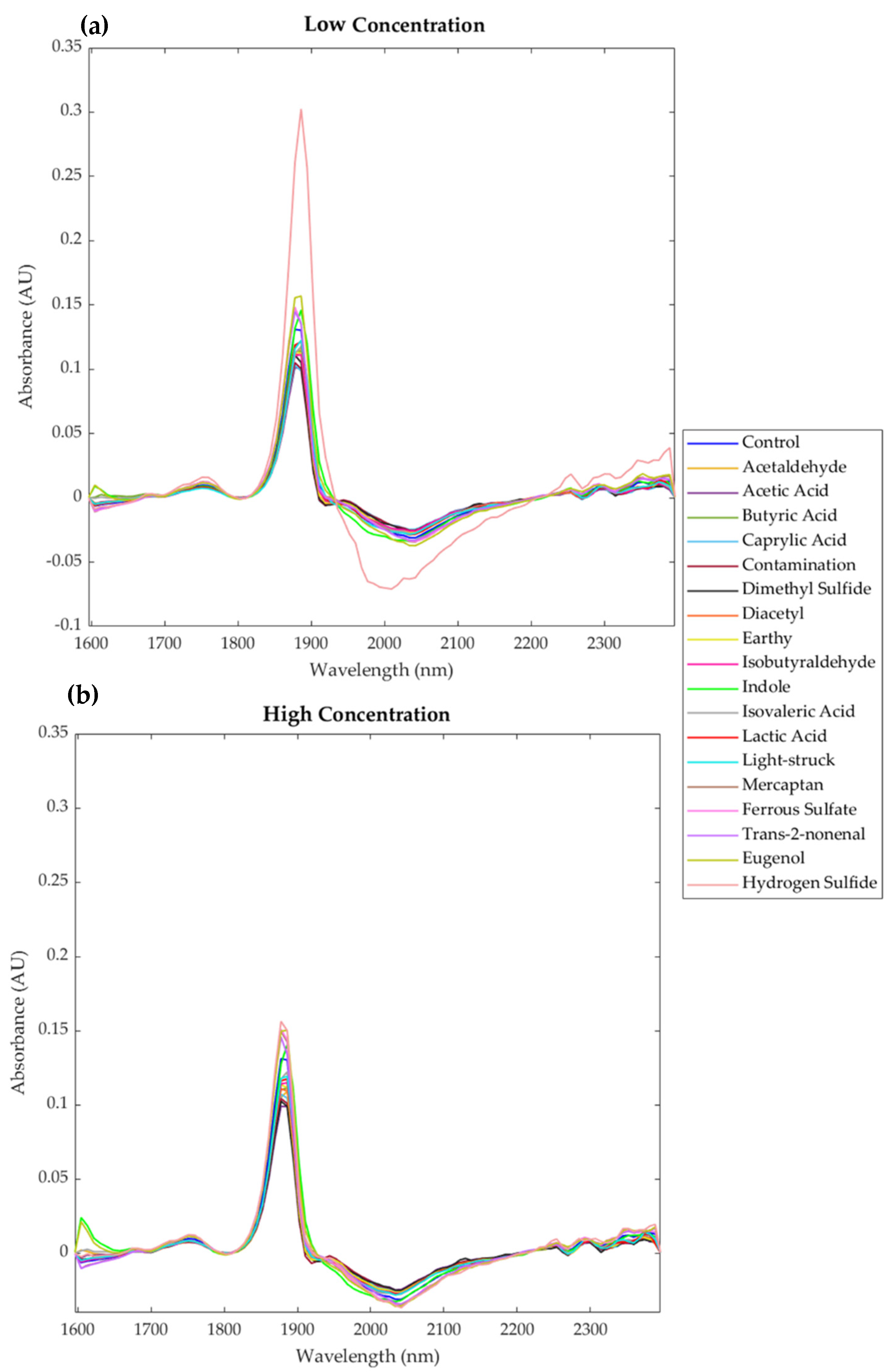
Figure 2 shows the curves of the NIR raw values for the control and each fault tested for low and high concentrations. It can be observed that the overtones were similar for both low and high concentrations; however, the absorbance values were different. The overtones found for all samples are within the 1900 and 2000 nm and >2250 nm. On the other hand, in Figure 3, which shows the absorbance values for the first derivative transformation, the overtones were enhanced within the 1850–1905 nm and 1950–2140 nm ranges. In both Figures, it could be observed that the sample with hydrogen sulfide at low concentration had higher absorbance values than with the high concentration.
Figure 4 shows the stacked bar graphs depicting the ANOVA results, mean values, and error bars based on the standard error of each e-nose sensor and each beer sample for low and high concentrations. It can be observed that there were significant differences (p < 0.05) between samples for all sensors. The MQ3 (alcohol) presented the highest voltage values for all samples, followed by the MQ4 (CH4). The Mercaptan sample was the highest in alcohol gas release for the low concentration, while acetic acid presented the lowest signal. Lactic acid and light-struck had the highest signal for MQ4 (CH4) and MQ137 (ammonia). On the other hand, for the high concentration samples, Eugenol was the highest in voltage for MQ3, MQ4, MQ135, and MQ137, while Indole was the lowest for MQ3. Even though a beer sample with H2S was evaluated, it did not have the highest signal for the MQ136 sensor (H2S) in both concentrations.
Figure 5 shows the correlation matrix for the e-nose outputs and beer spiked with faults. It can be observed that MQ3 had positive and low but significant (p < 0.05) differences with caprylic acid (r = 0.16), mercaptan (r = 0.11), trans-2-nonenal and Eugenol (r = 0.14), and negative correlations with acetaldehyde (r = −0.23) and indole (r = −0.10). The MQ136 (H2S) sensor had a positive correlation with trans-2-nonenla (r = 0.23), eugenol (r = 0.28), and hydrogen sulfide (r = 0.10), and a negative correlation with acetaldehyde (r = −0.28). Furthermore, Eugenol presented positive correlations with MQ4 (r = 0.35), MQ8 (r = 0.33), MQ135 (r = 0.34), and MQ137 (r = 0.18). The sample with contamination fault had positive correlations with acetic acid (r = 0.69) and diacetyl (r = 0.69).
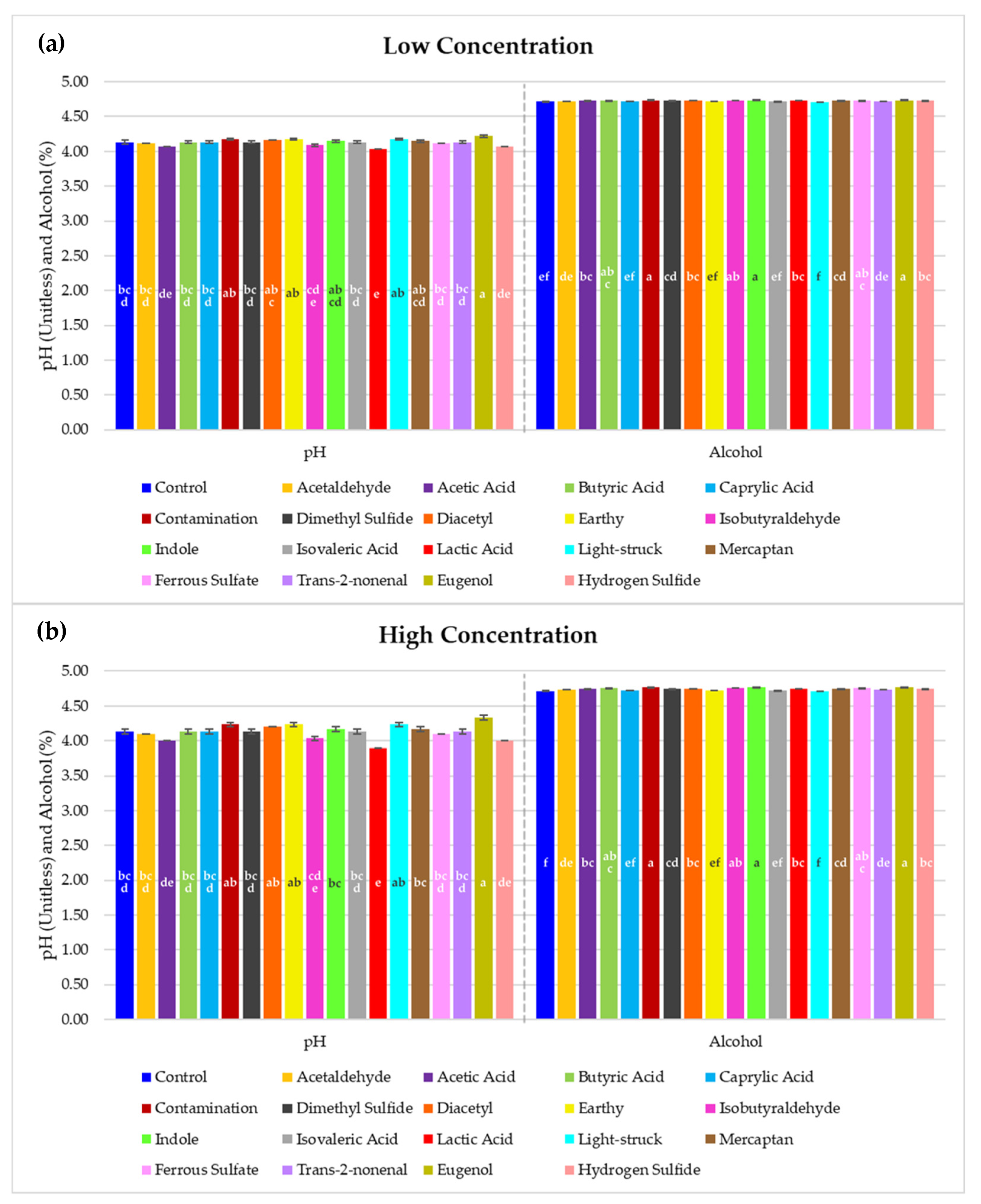
Figure 6 shows significant differences (p < 0.05) between samples for pH and alcohol content for low and high concentration treatments. It can be observed that at both low and high concentrations, the beer with eugenol had the highest pH (Low: 4.22; High: 4.33), while the sample with lactic acid presented the lowest pH (Low: 4.03; High: 3.90), which differed from the control (4.13). On the other hand, the sample with Eugenol and low and high concentration had the highest alcohol content (Low: 4.73; High: 4.77), while the light-stuck sample had the lowest alcohol content (Low and High: 4.71%), which was similar to the control (4.71%).
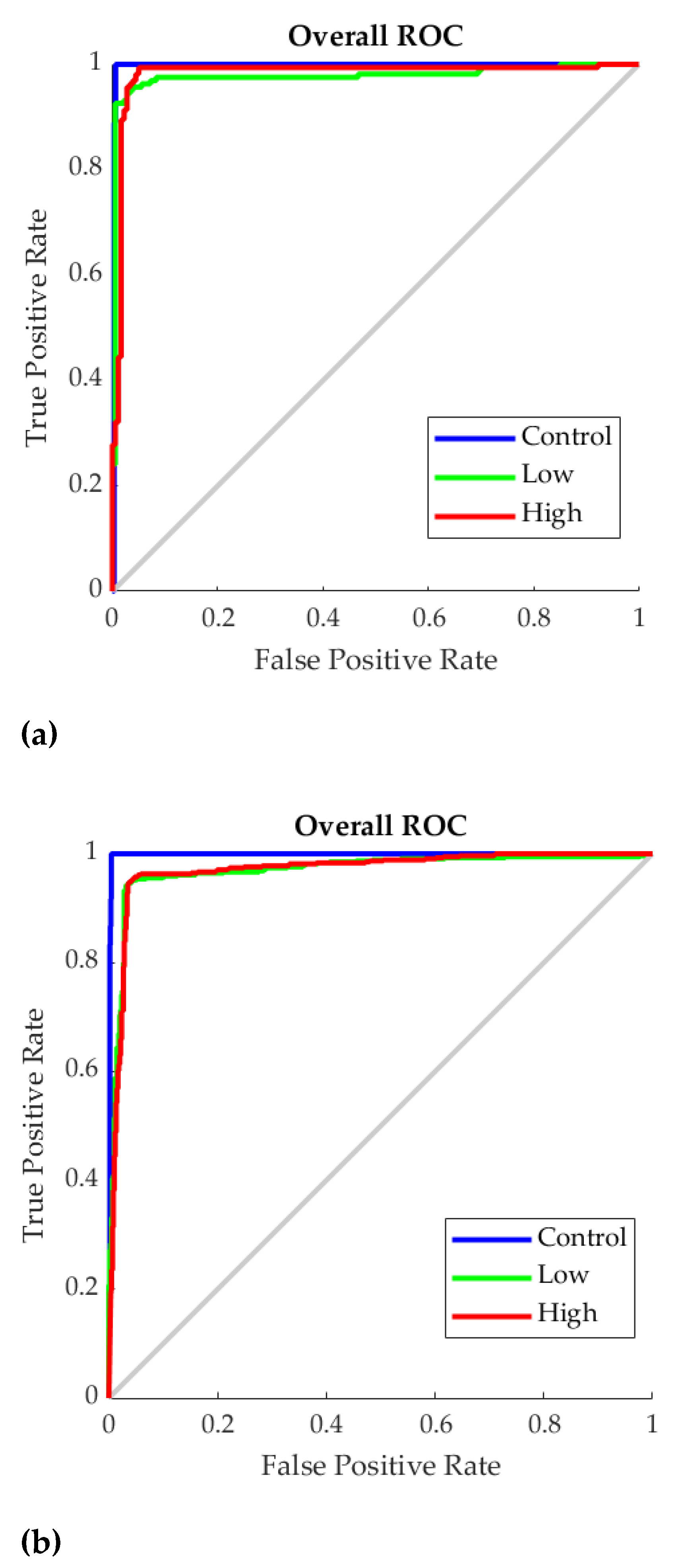
Table 3 shows that both Model 1 (NIR inputs) and Model 2 (e-nose inputs) had high overall accuracy (>95%) to classify the beer samples into control, low and high concentrations of faulty aromas. None of these models was under- or overfitted because their training MSE values were lower than the testing stage, which indicates they gave a high performance. Furthermore, in their receiver operating characteristic (ROC) curves (Figure 7), it can be seen that the three classifications in the two models had very high sensitivity (true positive rate; >0.94). It can be observed that the lowest sensitivity for Models 1 and 2 was the low concentration (0.94 and 0.95, respectively).
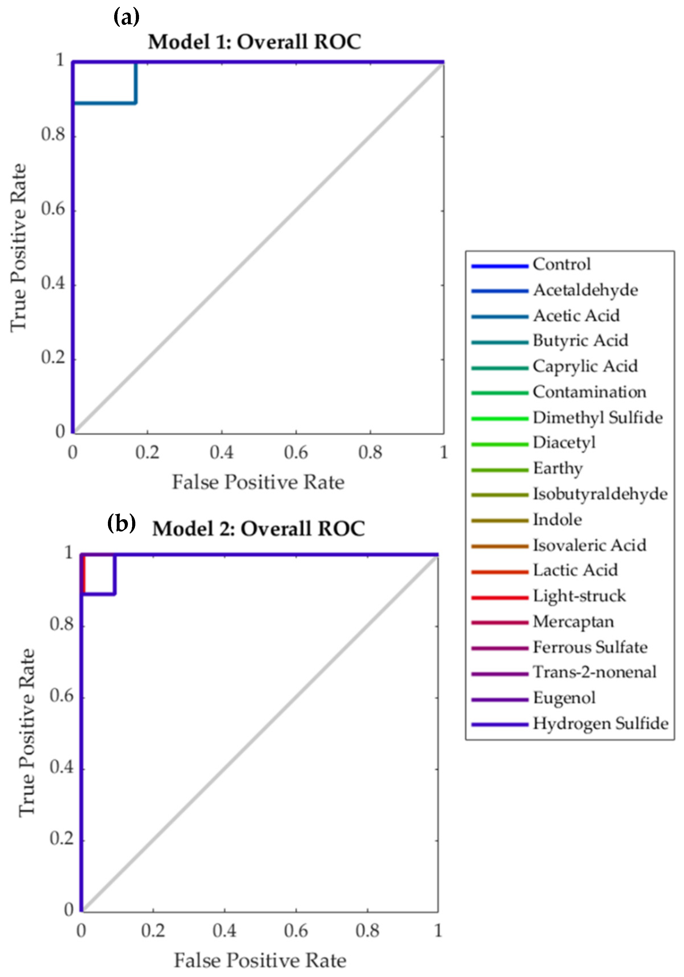
Table 4 shows that Models 3 (low concentration) and 4 (high concentration) developed using the NIR absorbance values as inputs had high overall accuracy with 99% and 98%, respectively. None of the models presented any signs of under- or overfitting as the training performance (Models 3 and 4: MSE < 0.001) was lower than the testing (Model 3: MSE = 0.003; Model 4: MSE = 0.005). Figure 8 depicts the ROC curves for Models 3 and 4, in which it can be observed that all of the classification categories had high sensitivity (>0.89). In Model 3, acetic acid and H2S were the lowest in sensitivity (0.89), while in Model 4, the lowest were samples earthy, light-struck, and H2S (0.89).
Table 5 shows that Models 5 (low concentration) and 6 (high concentration) developed using the e-nose outputs as inputs had high overall accuracy (97% and 96%, respectively). In both, Models 5 and 6, the training performance (Models 5 and 6: MSE < 0.001) was lower than the testing (Model 5: MSE = 0.009; Model 6: MSE = 0.011). Based on the ROC curves (Figure 9), all classification categories had high sensitivity (>0.87), with caprylic acid being the lowest sensitivity in Model 5 (0.90) and diacetyl and ferrous sulfate in Model 6 (0.87).

4. Discussion

4.1. Near-Infrared Spectroscopy (NIR)

The NIR range used in this study includes the aromatic overtones, which corresponded to 1596–2396 nm. This NIR range has been used in previous studies to characterize and model different volatile aromatic compounds in beers [19,25,32] and wine [33,34]. The major raw NIR peaks shown for all samples were in 1900–2000 nm and >2300 nm (Figure 2), which correspond to overtones of compounds such as carboxylic acid, pOH, water, amides, alcohol, proteins, and carbohydrates [35]. After a first derivative transformation (Figure 3), several other peaks and valleys were enhanced, such as other water overtones, thiols, and starch, all of which are found in beer [35]. The major differences in the latter case were observed between 1600 and 1700 nm, where aromatic compounds and alkyls can be found, at 1890 nm as the major peak, which corresponds to carboxylic acid, which may be present in beer samples in the form of different compounds such as acetic and lactic acids, and may derivate into esters, which are responsible for different aromas in beer [29,35], and between 1950 and 2150 nm, where proteins, amides, alcohol, and sucrose are found [35,36]. Interestingly, one off-aroma addition was significantly different compared to the rest (hydrogen sulfide) for low concentrations (Figure 3a) but not for high concentrations used (Figure 3b). The latter effect may be related to the initial interaction between the H2S compound and other minerals in the beer, increasing the chemical fingerprint in the specific overtones, which decrease at higher H2S concentrations [37]. These patterns and differences between the chemical fingerprint for samples with different fault additions are assessed using machine learning for discrimination purposes and potential identification and classification using ANN modeling techniques.

4.2. Low-Cost e-Nose and Beer Chemometrics

The low-cost e-nose used was preliminarily tested on different commercial beers for ML classification purposes and determination of aroma profiles compared to gas chromatography [29]. The same e-nose was successfully used to assess and quantify smoke taint compounds in wine [38]. The variation of the e-nose sensors response after the addition of fault compounds is significant for most of the sensors (Figure 4) and with differences between variations for low concentrations (Figure 4a) compared to high concentrations (Figure 4b) of faults, which helps to justify the classifications performed by the machine learning modeling techniques.
The latter is also supported by the general correlation matrix analysis (Figure 5) between all the fault compound additions and the different e-nose sensors. More negative and statistically significant correlations (p < 0.05) were found between acetaldehyde and most sensors except for MQ7 and with a positive correlation with MG811. The negative correlations between acetaldehyde and sensors sensitive to alcohol may be associated with the fact that acetaldehyde is often produced from the oxidation of ethanol [8,39]. The same trends were shown for sensor MQ4 (CH4) and acetic acid; this negative correlation was found in breweries, where CH4 production decreased acetic acid formation [40]. As expected, contamination was positively correlated with diacetyl, and butyric acid was formed when the latter two are mixed. Furthermore, Indole was negatively correlated to MQ3, MQ137, MQ8, and MQ135. The negative correlation between Indole and the sensors sensitive to alcohol may be since Indole is formed by coliform bacteria, which is eliminated with the presence of alcohol; therefore, at higher alcohol, lower indole production [8]. Furthermore, as expected, hydrogen sulfide was positively correlated with MQ136 (H2S) sensor; however, the correlation, although positive, was weak due to the sensitivity (1–100 mg L−1) of the sensor [29], which is higher than the concentrations used in the samples for this study (0.03 and 0.07 mg L−1). The rest of the fault compounds were positively correlated at different levels with most of the sensors.
There are fewer variations concerning basic chemometrics, such as pH and alcohol levels, which can be explained through the interactions of fault compounds (Figure 6), especially at high concentrations (Figure 6b), which were more significant for the case of pH compared to alcohol concentration. As expected, an increase in alcohol and a decrease in pH can be observed in samples with compounds that have an alcohol group and acidic faults, respectively.

4.3. Supervised Machine Learning Classification Models and Deployment

Models 1 and 2 were developed to determine whether the beers are a control (no faults), low, or high concentration of faults. This will indicate which model should be used to further predict the specific fault present in the sample: Models 3 (low concentration) or 4 (high concentration) for NIR and Models 5 (low concentration) or 6 (high concentration) for e-nose.
All six models based on NIR and e-nose resulted in high accuracies (>95% for NIR and e-nose, Models 1 and 2; >98% for NIR Models 3 and 4, and >96% for e-nose, Models 5 and 6). These accuracies and performances are consistent with those presented in previous studies using NIR and e-nose for beer to assess aroma compounds and for the classification of commercial beers [22,29].
In terms of practicality, even though the e-nose models have lower performance than the NIR models, the low-cost and integrability nature of the e-nose makes it more flexible for deployment to be added to different brewing processes with automated data acquisition and interpretation through AI. The e-nose processed data can be readily available to brewers for decision-making using wireless data transmission through the Internet of Things (IoT) [41,42]. On the contrary, the commercial NIR instrument used in this study cannot be integrated with AI as it can only incorporate models based on partial least squares (PLS), which have the limitation of assessing regression levels of single compounds per model for manual and punctual measurements, also requiring a trained operator for the instrument usage, data acquisition, handling, and interpretation. Furthermore, additional software is required for PLS modeling and integration with the NIR at a considerable cost.
Another advantage of the e-nose and AI method proposed compared to NIR is the implementation and deployment costs using the beforementioned data transmission and cloud processing using AI since it is based on numeric data transmission from the different voltage readings of sensors. The NIR instrument can be cost-prohibitive for craft brewing companies compared to the cost of the e-nose hardware, which corresponds to 2.5% of the NIR instrument.

5. Conclusions

The comparative accuracies of ML models developed for NIR and e-nose make the latter method cost-effective, reliable, and easy to deploy for craft, medium, and big brewing companies. The latter also allows the implementation and deployment of this method with the option of replication to assess multiple batches simultaneously. Due to the portability of new versions of e-noses considering local data storage and analysis using local and inexpensive microprocessors (i.e., Jetson® from NVIDIA, Arduino® or Raspberry Pi ®), these could be added to robots such as the RoboBEER for quality traits and consumer perception assessment using AI. Further studies are required to model fault assessment on different beer styles with more complex aroma profiles, such as lambic and within different stages of the brewing process. The results presented here are from a preliminary study on the integration of low-cost sensor technology and AI, and the models developed can be enriched with further data making the most of the learning capabilities of the ANN models considered.

Author Contributions

Conceptualization, C.G.V. and S.F.; data curation, C.G.V. and S.F.; formal analysis, C.G.V.; funding acquisition, C.H.-B.; investigation, C.G.V. and S.F.; methodology, C.G.V. and S.F.; project administration, C.G.V. and S.F.; resources, C.G.V. and S.F.; software, C.G.V. and S.F.; validation, C.G.V. and S.F.; visualization, C.G.V. and S.F.; writing—original draft, C.G.V. and S.F.; writing—review and editing, C.G.V., S.F., and C.H.-B. All authors have read and agreed to the published version of the manuscript.

Funding

This research was funded by the Mexican Beer and Health Council (Consejo de Investigación sobre Salud y Cerveza de México).

Institutional Review Board Statement

Not applicable.

Informed Consent Statement

Not applicable.

Data Availability Statement

Data and intellectual property belong to The University of Melbourne; any sharing needs to be evaluated and approved by the university.

Acknowledgments

The authors would like to acknowledge Ranjith R. Unnithan, and Bryce Widdicombe from the School of Engineering, Department of Electrical and Electronic Engineering of The University of Melbourne for their collaboration in the electronic nose development.

Conflicts of Interest

The authors declare no conflict of interest.

References

  1. Spedding, G.; Aiken, T. Sensory analysis as a tool for beer quality assessment with an emphasis on its use for microbial control in the brewery. In Brewing Microbiology; Elsevier: Amsterdam, The Netherlands, 2015; pp. 375–404. [Google Scholar]
  2. Amerine, M.A.; Pangborn, R.M.; Roessler, E.B. Principles of Sensory Evaluation of Food; Elsevier: Amsterdam, The Netherlands, 2013. [Google Scholar]
  3. Lawless, H.T. Quantitative Sensory Analysis: Psychophysics, Models and Intelligent Design; Wiley: Hoboken, NJ, USA, 2013. [Google Scholar]
  4. Ristic, R.; Danner, L.; Johnson, T.; Meiselman, H.; Hoek, A.; Jiranek, V.; Bastian, S. Wine-related aromas for different seasons and occasions: Hedonic and emotional responses of wine consumers from Australia, UK and USA. Food Qual. Prefer. 2019, 71, 250–260. [Google Scholar] [CrossRef]
  5. Ragazzo-Sanchez, J.; Chalier, P.; Chevalier-Lucia, D.; Calderon-Santoyo, M.; Ghommidh, C. Off-flavours detection in alcoholic beverages by electronic nose coupled to GC. Sens. Actuators B Chem. 2009, 140, 29–34. [Google Scholar] [CrossRef]
  6. Díaz, A.; Ventura, F.; Galceran, M.T. Identification of 2, 3-butanedione (diacetyl) as the compound causing odor events at trace levels in the Llobregat River and Barcelona’s treated water (Spain). J. Chromatogr. A 2004, 1034, 175–182. [Google Scholar] [CrossRef] [PubMed]
  7. Miller, G.H. Whisky Science: A Condensed Distillation; Springer: Berlin/Heidelberg, Germany, 2019. [Google Scholar]
  8. Barnes, T. The complete beer fault guide v. 1.4. January 2011. Available online: https://londonamateurbrewers.co.uk/wp-content/uploads/2015/05/Complete_Beer_Fault_Guide.pdf (accessed on 10 June 2021).
  9. Cravero, M.C.; Bonello, F.; Pazo Alvarez, M.d.C.; Tsolakis, C.; Borsa, D. The sensory evaluation of 2, 4, 6-trichloroanisole in wines. J. Inst. Brew. 2015, 121, 411–417. [Google Scholar] [CrossRef]
  10. Wray, E. Common faults in beer. In The Craft Brewing Handbook; Elsevier: Amsterdam, The Netherlands, 2020; pp. 217–246. [Google Scholar]
  11. Mander, L.; Liu, H.-W. Comprehensive Natural Products II: Chemistry and Biology; Elsevier: Amsterdam, The Netherlands, 2010; Volume 1. [Google Scholar]
  12. Pomeroy, R.D.; Cruse, H. Hydrogen sulfide odor threshold. J. Am. Water Work. Assoc. 1969, 61, 677. [Google Scholar] [CrossRef]
  13. World Health Organization. WHO Guidelines for Drinking Water Quality, 2nd ed.; WHO: Geneva, Switzerland, 1996. [Google Scholar]
  14. Viejo, C.G.; Fuentes, S.; Howell, K.; Torrico, D.; Dunshea, F.R. Robotics and computer vision techniques combined with non-invasive consumer biometrics to assess quality traits from beer foamability using machine learning: A potential for artificial intelligence applications. Food Control 2018, 92, 72–79. [Google Scholar] [CrossRef]
  15. Viejo, C.G.; Fuentes, S. Beer Aroma and Quality Traits Assessment Using Artificial Intelligence. Fermentation 2020, 6, 56. [Google Scholar] [CrossRef]
  16. Wilson, C.; Threapleton, L. Application of artificial intelligence for predicting beer flavours from chemical analysis. In Proceedings of the 29th European Brewery Convention Congress, Dublin, Ireland, 17–22 May 2003; pp. 17–22. [Google Scholar]
  17. Geilings, B. Using Artificial Intelligence to Positively Impact the Beer Brewing Process. Bachelor’s Thesis, Haaga-Helia University of Applied Sciences, Helsinki, Finland, 2021. [Google Scholar]
  18. Viejo, C.G.; Fuentes, S.; Li, G.; Collmann, R.; Condé, B.; Torrico, D. Development of a robotic pourer constructed with ubiquitous materials, open hardware and sensors to assess beer foam quality using computer vision and pattern recognition algorithms: RoboBEER. Food Res. Int. 2016, 89, 504–513. [Google Scholar] [CrossRef]
  19. Gonzalez Viejo, C.; Fuentes, S.; Torrico, D.; Howell, K.; Dunshea, F.R. Assessment of beer quality based on foamability and chemical composition using computer vision algorithms, near infrared spectroscopy and machine learning algorithms. J. Sci. Food Agric. 2018, 98, 618–627. [Google Scholar] [CrossRef]
  20. Vann, L.; Layfield, J.B.; Sheppard, J.D. The application of near-infrared spectroscopy in beer fermentation for online monitoring of critical process parameters and their integration into a novel feedforward control strategy. J. Inst. Brew. 2017, 123, 347–360. [Google Scholar] [CrossRef] [Green Version]
  21. Fox, G. The brewing industry and the opportunities for real-time quality analysis using infrared spectroscopy. Appl. Sci. 2020, 10, 616. [Google Scholar] [CrossRef] [Green Version]
  22. Gonzalez Viejo, C.; Fuentes, S. Low-Cost Methods to Assess Beer Quality Using Artificial Intelligence Involving Robotics, an Electronic Nose, and Machine Learning. Fermentation 2020, 6, 104. [Google Scholar] [CrossRef]
  23. Voss, H.G.J.; Mendes Júnior, J.J.A.; Farinelli, M.E.; Stevan, S.L. A Prototype to Detect the Alcohol Content of Beers Based on an Electronic Nose. Sensors 2019, 19, 2646. [Google Scholar] [CrossRef] [PubMed] [Green Version]
  24. Ghasemi-Varnamkhasti, M.; Mohtasebi, S.; Rodriguez-Mendez, M.; Lozano, J.; Razavi, S.; Ahmadi, H. Potential application of electronic nose technology in brewery. Trends Food Sci. Technol. 2011, 22, 165–174. [Google Scholar] [CrossRef]
  25. Viejo, C.G.; Torrico, D.D.; Dunshea, F.R.; Fuentes, S. Development of Artificial Neural Network Models to Assess Beer Acceptability Based on Sensory Properties Using a Robotic Pourer: A Comparative Model Approach to Achieve an Artificial Intelligence System. Beverages 2019, 5, 33. [Google Scholar] [CrossRef] [Green Version]
  26. Santos, J.P.; Lozano, J. Real time detection of beer defects with a hand held electronic nose. In Proceedings of the 2015 10th Spanish Conference on Electron Devices (CDE), Madrid, Spain, 11–13 February 2015; pp. 1–4. [Google Scholar]
  27. Sanaeifar, A.; ZakiDizaji, H.; Jafari, A.; de la Guardia, M. Early detection of contamination and defect in foodstuffs by electronic nose: A review. TrAC Trends Anal. Chem. 2017, 97, 257–271. [Google Scholar] [CrossRef]
  28. Pornpanomchai, C.; Suthamsmai, N. Beer classification by electronic nose. In Proceedings of the 2008 International Conference on Wavelet Analysis and Pattern Recognition, Hong Kong, China, 30–31 August 2008; pp. 333–338. [Google Scholar]
  29. Gonzalez Viejo, C.; Fuentes, S.; Godbole, A.; Widdicombe, B.; Unnithan, R.R. Development of a low-cost e-nose to assess aroma profiles: An artificial intelligence application to assess beer quality. Sens. Actuators B Chem. 2020, 308, 127688. [Google Scholar] [CrossRef]
  30. Gonzalez Viejo, C.; Tongson, E.; Fuentes, S. Integrating a Low-Cost Electronic Nose and Machine Learning Modelling to Assess Coffee Aroma Profile and Intensity. Sensors 2021, 21, 2016. [Google Scholar] [CrossRef] [PubMed]
  31. Perez, C. Big Data and Deep Learning. Examples with Matlab; Lulu Press, Inc: Morrisville, NC, USA, 2020. [Google Scholar]
  32. Gonzalez Viejo, C.; Torrico, D.D.; Dunshea, F.R.; Fuentes, S. Emerging Technologies Based on Artificial Intelligence to Assess the Quality and Consumer Preference of Beverages. Beverages 2019, 5, 62. [Google Scholar] [CrossRef] [Green Version]
  33. Smyth, H.; Cozzolino, D.; Cynkar, W.; Dambergs, R.; Sefton, M.; Gishen, M. Near infrared spectroscopy as a rapid tool to measure volatile aroma compounds in Riesling wine: Possibilities and limits. Anal. Bioanal. Chem. 2008, 390, 1911–1916. [Google Scholar] [CrossRef]
  34. Ferrer-Gallego, R.; Hernández-Hierro, J.M.; Rivas-Gonzalo, J.C.; Escribano-Bailón, M.T. Evaluation of sensory parameters of grapes using near infrared spectroscopy. J. Food Eng. 2013, 118, 333–339. [Google Scholar] [CrossRef]
  35. Burns, D.A.; Ciurczak, E.W. Handbook of Near-Infrared Analysis; CRC press: Boca Raton, FL, USA, 2007. [Google Scholar]
  36. Osborne, B.G.; Fearn, T.; Hindle, P.H. Practical NIR Spectroscopy with Applications in Food and Beverage Analysis; Longman Scientific and Technical: London, UK, 1993. [Google Scholar]
  37. Brenner, M.; Khan, A.; Bernstein, L. Formation and Retention of Free H2S and of Free Volatile Thiols during Beer Fermentation. In Proceedings of the Annual Meeting-American Society of Brewing Chemists, St. Paul, MN, USA, 1 December 1975; pp. 82–93. [Google Scholar]
  38. Fuentes, S.; Summerson, V.; Gonzalez Viejo, C.; Tongson, E.; Lipovetzky, N.; Wilkinson, K.L.; Szeto, C.; Unnithan, R.R. Assessment of Smoke Contamination in Grapevine Berries and Taint in Wines Due to Bushfires Using a Low-Cost E-Nose and an Artificial Intelligence Approach. Sensors 2020, 20, 5108. [Google Scholar] [CrossRef] [PubMed]
  39. Pesselman, R.L.; Meshbesher, T.M.; Floyd, S.D.; Langer, S.H. Electrogenerative oxidation of ethanol to acetaldehyde. Chem. Eng. Commun. 1985, 38, 265–273. [Google Scholar] [CrossRef]
  40. Gomes, M.M.; Sakamoto, I.K.; Rabelo, C.A.B.S.; Silva, E.L.; Varesche, M.B.A. Statistical optimization of methane production from brewery spent grain: Interaction effects of temperature and substrate concentration. J. Environ. Manag. 2021, 288, 112363. [Google Scholar] [CrossRef] [PubMed]
  41. Violino, S.; Figorilli, S.; Costa, C.; Pallottino, F. Internet of beer: A review on smart technologies from mash to pint. Foods 2020, 9, 950. [Google Scholar] [CrossRef]
  42. Betts, B. Brewing up: A technology revolution. Eng. Technol. 2016, 11, 54–57. [Google Scholar] [CrossRef]
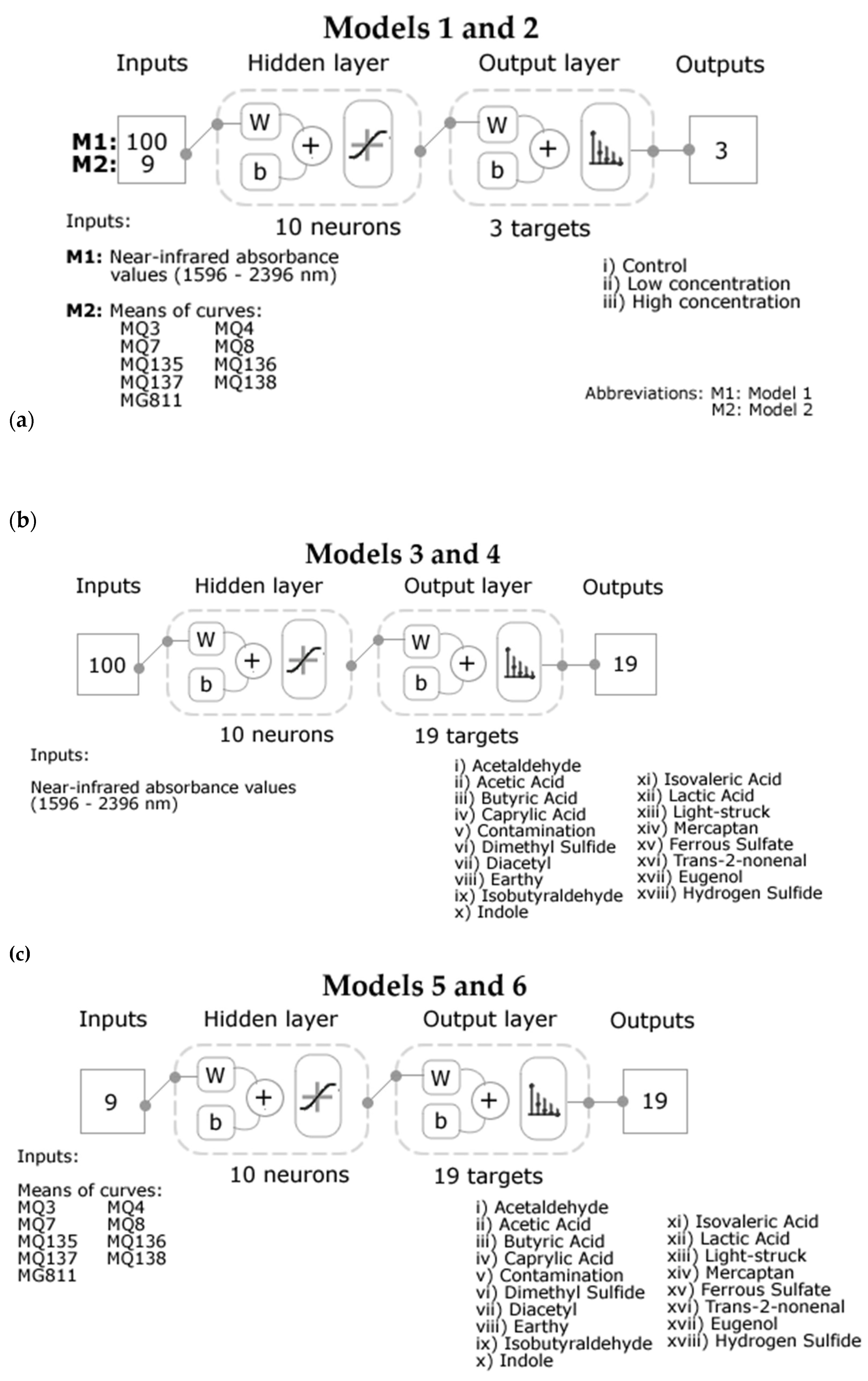
Figure 1. Diagrams of the two-layer feedforward models with a tan-sigmoid function in the hidden layer and a Softmax function in the output layer for (a) Models 1 (Near-infrared inputs), and 2 (electronic nose inputs), (b) Models 3 (low concentration) and 4 (high concentration), and (c) Models 5 (low concentration) and 6 (high concentration). Abbreviations: W: weights; b: bias.
Fermentation 07 00117 g001
Figure 2. Near-infrared curves for all beer samples using the raw absorbance values at (a) low and (b) high concentrations.
Fermentation 07 00117 g002
Figure 3. Near-infrared curves for all beer samples using the first derivative of the absorbance values at (a) low and (b) high concentrations.
Fermentation 07 00117 g003
Figure 4. Stacked bar graphs for (a) low and (b) high concentrations showing the mean voltage values obtained from the electronic nose sensors. Error bars are based on standard error. Different letters depict significant differences (p < 0.05) between samples for each sensor based on the Tukey honest significant difference (HSD) post-hoc test.
Fermentation 07 00117 g004
Figure 5. Matrix showing the significant (p < 0.05) correlations between the electronic nose sensors and the beer samples spiked with faults. Color bar represents the positive correlations on the blue side and negative correlations on the yellow side.
Fermentation 07 00117 g005
Figure 6. Bar graphs of the pH and alcohol mean values for (a) low and (b) high concentration treatment. Error bars are based on standard error. Different letters depict significant differences (p < 0.05) between samples for each sensor based on the Tukey honest significant difference (HSD) post-hoc test.
Fermentation 07 00117 g006
Figure 7. Receiver operating characteristic (ROC) curves of the models developed using (a) near-infrared (Model 1) and (b) electronic nose (Model 2) values as inputs to classify beers according to the concentration of faults present in them (control, low and high concentration).
Fermentation 07 00117 g007
Figure 8. Receiver operating characteristic (ROC) curves of the (a) low (Model 3) and (b) high (Model 4) concentration samples to classify beers according to the faults present in them using the near-infrared absorbance values as inputs.
Fermentation 07 00117 g008
Figure 9. Receiver operating characteristic (ROC) curves for the (a) low (Model 5) and (b) high (Model 6) concentration samples to classify beers according to the faults present in them using the electronic nose outputs as inputs.
Fermentation 07 00117 g009
Table 1. Description and concentrations of typical beer faults (off-aromas/flavors).
Common NameChemical CompoundAroma/FlavorOriginContamination StageDetection Threshold in Water (mg L−1)Typical
Concentration in Beer (mg L−1)
Spoilage Concentration in Beer (mg L−1)References
Diacetyl2,3-butanedioleButterLow levels of valine in wort Microbial contaminationWort5 × 10−48 × 10−3–0.600.25[5,6,7,8]
TCA *2,4,6-trichloroanisoleMust taint/
Moldy
Contaminated ingredients or other material (packaging)Ageing
Storage
3 × 10⁻⁸–200 × 10−8Absent0.02[5,7,9]
Acetic acidAcetic acidSour/Vinegar/
Tangy
Spoilage bacteria
Wild yeast
Fermentation
Conditioning
0.1030–20060.0–120.0[7,8,10]
Lactic acidLactic acidSour/Sour milk/TartSpoilage bacteriaMashing
Secondary fermentation
0.040.20–1.50140[8,10]
H2SHydrogen sulfideRotten eggsRaw material
Yeast contamination
Fermentation1 × 10−5–10 × 10−5≤1 × 10−34 × 10−3[8,10,11,12]
DMSDimethyl sulfideSweet corn/
Onion/Rotten vegetables
Microbial contaminationWort boiling/cooling3.3 × 10−70.01–0.150.40[8,10]
PaperyTrans-2-nonenalCardboard/
Oxidized
Oxidation
Staling
Fermentation
Storage
8 × 10⁻⁸< 5 × 10−54 × 10−4[8,10]
Isovaleric acidIsovaleric acidCheesy/Rancid/
Sweaty feet
Old/Oxidized hops
Process faults
Boiling
Ageing
4.9 × 10⁻⁴≤ 0.201.00[7,8,10]
Earthy2-Ethyl fencholSoil/Compost/
Moldy
Microbial contaminationPackaging5 × 10−3 **Absent5 × 10−3[8]
AcetaldehydeAcetaldehydeGreen apple/
Bready/Grass
Staling
Microbial contamination
Poor yeast health
Fermentation
Storage
2.5 × 10⁻⁵–6.5 × 10−52.00–15.020.0[7,8]
ButyricButyric acidBaby vomit/ Putrid/Rancid butterMicrobial contamination
Ageing
Wort production
Packaging/Storage
2.4 × 10−30.50–1.503.00[7,8]
CaprylicCaprylic acidGoat/Soap/
Sweaty
Microbial contamination
Yeast breakdown
Maturation0.013 **2.00–8.0010.0[7,8]
MercaptanEthanethiolDrains/SewerAutolysis
Poor yeast health
Fermentation
Ageing
1.7 × 10⁻⁶ **0.00–5 × 10−31 × 10−3[7,8]
SpicyEugenolCloveMicrobial contamination
Wild yeast
Oxidation
Ageing7.1 × 10−70.01–0.030.40[7,8]
MetallicFerrous sulfateMetal/Blood/ Coin/IronWater sources
Non-passivated vessels
Any brewing stage1.00–1.50 **≤ 0.501.00[8]
GrainyIsobutyraldehydeCereal husks/ Green malt/ Raw grainExcessive run-off
Insufficient boiling
Wort boiling4.9 × 10−71 × 10−3–0.021.00–2.50[7,8]
IndoleIndoleFarm/Barnyard/ Fecal/Pig-likeMicrobial contaminationFermentation5 × 10−3 **< 5 × 10−30.01–0.02[8]
Light-struck2-Methyl-2-butene-1-thiolFecal/Skunky/ SulfuryClear or green bottlesStorage4 × 10−6 **1 × 10⁻⁶–5 × 10−65.00–30.00[8]
Bromophenol *BromophenolInky/Museum-like/Old electronicsProcess/Equipment faults
Contaminated raw material
Any brewing stage3 × 10−9Absent1.3 × 10−3[7,8]
Catty *p-Methane-8-thiol-3-oneOxidized/tomcat urineHops
Contaminated raw material
Ageing
Packaging
1.5 × 10⁻⁵ **Absent1.5 × 10−5[8]
Plastic *StyreneBurning plastic/ ChemicalBrewing equipment and packaging material contaminationAny brewing stage0.02Absent0.02[8,13]
* Compounds not studied in this research. ** Detection threshold in beer as it has not been reported in water.
Table 2. Compounds used as off-flavors/aromas (faults) to spike beer samples and the concentrations used for training purposes according to human detection thresholds.
NumberFaultFlavor/Aroma *Concentration (Low; mg L−1)Concentration (High; mg L−1)
1AcetaldehydeGreen apple, cut grass19.545.0
2Acetic AcidVinegar156360
3Butyric AcidPutrid, baby vomit3.257.50
4Caprylic AcidSoapy, wax, fatty13.731.5
5Contamination
(Acetic Acid + Diacetyl)
Sour, buttery156361
6Dimethyl SulfideCooked vegetables0.170.40
7Diacetyl
(2,3-Butanediol)
Butter, butterscotch0.260.60
8Earthy
(2-Ethyl fenchol)
Soil6.5 × 10−30.02
9IsobutyraldehydeGrainy, husk, nut1.633.75
10IndoleFarm, barnyard0.240.55
11Isovaleric AcidCheese, sweaty socks, old hops2.606.00
12Lactic AcidSour milk173.33400
13Light-struck
(3-Methyl-2-butene-1-thiol)
Skunky, toffee, coffee2.6 × 10−46x10−4
14Mercaptan
(Ethanethiol)
Sewer, drains1.6 × 10−33.8 × 10⁻³
15Ferrous SulfateMetallic, blood1.633.75
16Trans-2-nonenalPapery, cardboard, oxidized8.7 × 10−42 × 10−3
17EugenolCloves, spicy0.050.12
18Hydrogen SulfideRotten Eggs0.030.07
* As described by the beer faults kit supplier (Siebel Institute, Chicago, IL, USA).
Table 3. Statistical results of the artificial neural network classification models developed using the near-infrared absorbance values Model 1 and electronic nose outputs (Model 2) as inputs to predict the concentration level. Abbreviations: MSE: means squared error.
StageSamplesAccuracyErrorPerformance
(MSE)
Model 1: Near-infrared inputs
Training239100%0.0%<0.001
Testing10385.4%14.6%0.08
Overall34295.6%4.4%-
Model 2: Electronic nose inputs
Training23998.5%1.5%0.01
Testing10387.7%12.3%0.08
Overall34295.3%4.7%-
Table 4. Statistical results of the artificial neural network classification models developed using the near-infrared absorbance values as inputs. Abbreviations: MSE: means squared error.
StageSamplesAccuracyErrorPerformance
(MSE)
Model 3: Near-infrared inputs—Low concentration
Training126100%0.0%<0.001
Testing5496.3%3.7%0.003
Overall18098.9%1.1%-
Model 4: Near-infrared inputs—High concentration
Training126100%0.0%<0.001
Testing5494.4%5.6%0.005
Overall18098.3%1.7%-
Table 5. Statistical results of the artificial neural network classification models developed using the electronic nose outputs as inputs. Abbreviations: MSE: means squared error.
StageSamplesAccuracyErrorPerformance
(MSE)
Model 5: Electronic nose inputs—Low concentration
Training42099.8%0.2%<0.001
Testing18090.0%10.0%0.009
Overall60096.8%3.2%-
Model 6: Electronic nose inputs—High concentration
Training420100%0.0%<0.001
Testing18087.2%12.8%0.011
Overall60096.2%3.8%-
Publisher’s Note: MDPI stays neutral with regard to jurisdictional claims in published maps and institutional affiliations.