Thermodynamic Equilibrium Study of Anaerobic Digestion through Helmholtz Equation of State

Abstract

The growing attention regarding a more sustainable future, and thus into energy recovery and waste reduction technologies, has intensified the interest towards processes which allow to exploit waste and biomasses to generate energy, such as the anaerobic digestion. Improving the efficiency of this industrial application is crucial to increase methane production, and is essential from the economic, environmental and safety point of view. This study focuses on the thermodynamic modelling of a steady-state reactor as a flash unit, in order to determine the best operating conditions to produce the maximum amount of pure bio-methane. To this purpose, a new hybrid approach based on the Peng–Robinson cubic equation of state and on the Multi-Parameter Helmholtz-Energy EoS has been proposed. The simulations, performed using the developed algorithm at temperatures between 20 and 55 °C and at pressure values between 0.3 atm and 1.5 atm, point out that the fugacity of the mixture evaluated with the proposed technique is much more accurate and reliable than the one calculated with the PR EoS. In addition, this research has shown not only that the purity and the production of the biogas can be optimised by working at mesophilic conditions and at pressure between 1 atm and 1.5 atm, but also that it is not convenient to operate in a temperature range of 42 °C–45 °C, since about 20 % more ${\mathrm{H}}_2\mathrm{S}$ goes into the exiting biogas, reducing the $\mathrm{C}{\mathrm{H}}_4$ amount and raising the post-treatment costs. Lastly, it has been seen that there is a significant water content in the vapour phase (∼5 %wt.), and this is a factor to be taken into account in order to improve the process.

1. Introduction

The Anaerobic Digestion (AD) process lays on the spontaneous decomposition of organic material, through the biological metabolism of facultative and obligate bacteria. The principal products of the process are biogas and digestate. The first is a vapour mix of highly volatile components as methane ($\mathrm{C}{\mathrm{H}}_4$) and carbon dioxide ($\mathrm{C}{\mathrm{O}}_2$). This is then used as an intermediate chemical or injected into a combustion unit to produce electric energy and the necessary heat to run the process [1]. The other is the digestate, a fangoviscous phase rich in water, minerals (i.e., potassium, phosphorous) and mineralised exhausted biomass [2]. This, after its stabilisation, is extensively used as conditioner and fertilizer of agricultural soils.

It is widely known that the relative compositions of methane and carbon dioxide in the biogas are rather relevant (50–70% for $\mathrm{C}{\mathrm{H}}_4$, 50–30% for $\mathrm{C}{\mathrm{O}}_2$) [3]. However, many other intermediates and products are obtained during the digestion process. Indeed, it is possible to define four kinetic reactions in the system [4]:

• Hydrolysis: This process depicts the chemical breakage of carbohydrate, protein and lipid polymeric linkages. Some research in the literature highlights the participation of cellulose, hemicellulose and lignin in the reaction [5,6], although their contribution is not as significant and can be overlooked. The end products are the monomers that make up the polymers, such as dextrose (sugar) from carbohydrates, amino acids from proteins and long-chain fatty acids from lipids.
• Acidogenesis: The previously obtained monomers are combined with hydrogen to form volatile fatty acids (VFA). The main components obtained include butyric acid, valeric acid, propionic acid and, under certain conditions, alcohols such as ethanol [7], as well as caproic acid [8] and lactic acid [9]. Meanwhile, ammonia and hydrogen sulphide are also formed in the liquid phase.
• Acetogenesis: A large amount of acetic acid is produced during this stage. However, some of it is also formed during acidogenesis. In fact, both processes are sometimes regarded to be as one. A large amount of hydrogen is produced, which is why it is also known as the dehydrogenating step [4].
• Methanogenesis: In the last step of the process, the principal product, methane, is produced. Two specific bacteria family are responsible for its formation: acetoclastic bacteria, which convert acetic acid into methane and carbon dioxide, and hydrogenotrophic bacteria, which instead convert hydrogen and carbon dioxide into methane and water. In particular conditions, also the decarboxylation of ethanol takes place, forming methane and other acetic acid. However, its contribution is quite lower relative to the other two reactions.

As said, during acidogenesis, the reduction of sulfate components happens, converting $\mathrm{S}{\mathrm{O}}_4^{2-}$ based compounds (deriving from amino acids) into $\mathrm{H}{\mathrm{S}}^{-}$, thus decreasing precious organic matter for methane production [10]. This is then released in the gas phase as ${\mathrm{H}}_2\mathrm{S}$. Being one of the most toxic compound produced during this process, it must be treated in order to be able to use the biogas for energy production. All the reactions are summarised in

Table 1. List of reactions happening in the anaerobic digestion.

Reaction Phase
Hydrolysis
(C6H10O5)${)}_n + n$H2O$\to n$C6H12O6$+ n$H2
Acidogenesis
${\mathrm{C}}_6{\mathrm{H}}_{12}{\mathrm{O}}_6 \to 2\mathrm{C}{\mathrm{H}}_3\mathrm{C}{\mathrm{H}}_2\mathrm{O}\mathrm{H}$$+ 2\mathrm{C}{\mathrm{O}}_2$
${\mathrm{C}}_6{\mathrm{H}}_{12}{\mathrm{O}}_6 + 2$${\mathrm{H}}_2$$\to 2\mathrm{C}{\mathrm{H}}_3\mathrm{C}{\mathrm{H}}_2\mathrm{C}\mathrm{O}\mathrm{O}\mathrm{H}$$+ 2{\mathrm{H}}_2\mathrm{O}$
${\mathrm{C}}_6{\mathrm{H}}_{12}{\mathrm{O}}_6 \to$$3\mathrm{C}{\mathrm{H}}_3\mathrm{C}\mathrm{O}\mathrm{O}\mathrm{H}$
Acetogenesis
${\mathrm{C}}_6{\mathrm{H}}_{12}{\mathrm{O}}_6 +$$2{\mathrm{H}}_2\mathrm{O}$$\to 2\mathrm{C}{\mathrm{H}}_3\mathrm{C}\mathrm{O}\mathrm{O}\mathrm{H}$$+ 2\mathrm{C}{\mathrm{O}}_2 + 3$${\mathrm{H}}_2$
$\mathrm{C}{\mathrm{H}}_3\mathrm{C}{\mathrm{H}}_2\mathrm{O}\mathrm{H}$$+ 2{\mathrm{H}}_2\mathrm{O}$$\to \mathrm{C}{\mathrm{H}}_3\mathrm{C}\mathrm{O}\mathrm{O}\mathrm{H} + 3$${\mathrm{H}}_2$
Methanogenesis
$\mathrm{C}{\mathrm{H}}_3\mathrm{C}\mathrm{O}\mathrm{O}\mathrm{H} \to$$\mathrm{C}{\mathrm{H}}_4$$+ \mathrm{C}{\mathrm{O}}_2$
$\mathrm{C}{\mathrm{O}}_2 + 4$${\mathrm{H}}_2$$\to \mathrm{C}{\mathrm{H}}_4$$+ 2{\mathrm{H}}_2\mathrm{O}$
2CH3CH2OH + CO2$\to$CH4 $+$ 2CH3COOH
Sulfate reduction
4H2 + ${\mathrm{SO}}_4^{2-} + {\mathrm{H}}^{+} \to \mathrm{H}{\mathrm{S}}^{-}$$+ 4$H2O
$\mathrm{C}{\mathrm{H}}_3\mathrm{C}\mathrm{O}{\mathrm{O}}^{-}$ + $\mathrm{S}{\mathrm{O}}_4^{2-} \to$2$\mathrm{H}\mathrm{C}{\mathrm{O}}_3^{-}$ + $\mathrm{H}{\mathrm{S}}^{-}$
$1.33$C3H5${\mathrm{O}}_2^{-} + {\mathrm{SO}}_4^{2-} \to 1.33$CH3COO−$+1.33$$\mathrm{H}\mathrm{C}{\mathrm{O}}_3^{-}$$+ 0.75$HS−$+ 1.33$H+
2C4H7O− + ${\mathrm{SO}}_4^{2-} \to 4$CH3COO− + HS− + H+

.

Being that the primary goal of the process is to produce as much methane as possible, this work focuses on the application of thermodynamic laws to evaluate and optimise the unit’s equilibrium conditions (steady-state), achieving the highest methane purity and, at the same time, the lowest byproducts content (i.e., $\mathrm{C}{\mathrm{O}}_2$, ${\mathrm{H}}_2\mathrm{S}$ and ${\mathrm{H}}_2\mathrm{O}$). It has already been demonstrated that thermodynamics can significantly improve microbial process comprehension and understand the true system’s environmental impact [11].

A special emphasis is given on the modelling of the reactor as a flash unit, where feed flowrate and starting composition are already established by the reactions reaching equilibrium conditions. As a result, the relative liquid–vapour species concentration was determined by varying the unit’s temperature and pressure within microbial-sensible ranges.

To describe and solve the unit equilibrium, the Multi-Parameter Helmholtz-Energy equation of state, that, for the sake of brevity, will be addressed as Helmholtz EoS, is employed, recovering all of the thermodynamic parameters of the species involved and defining the appropriate operative conditions for specific goals.

Moreover, a cubic-Helmholtz EoS hybrid approach is proposed to retrieve reliable values of the fugacity coefficients for the i-th species in mixture conditions. Consequently, also the best operative conditions, in terms of temperature and pressure, are seeked to produce the most pure biogas stream.

2. Mathematical Modelling

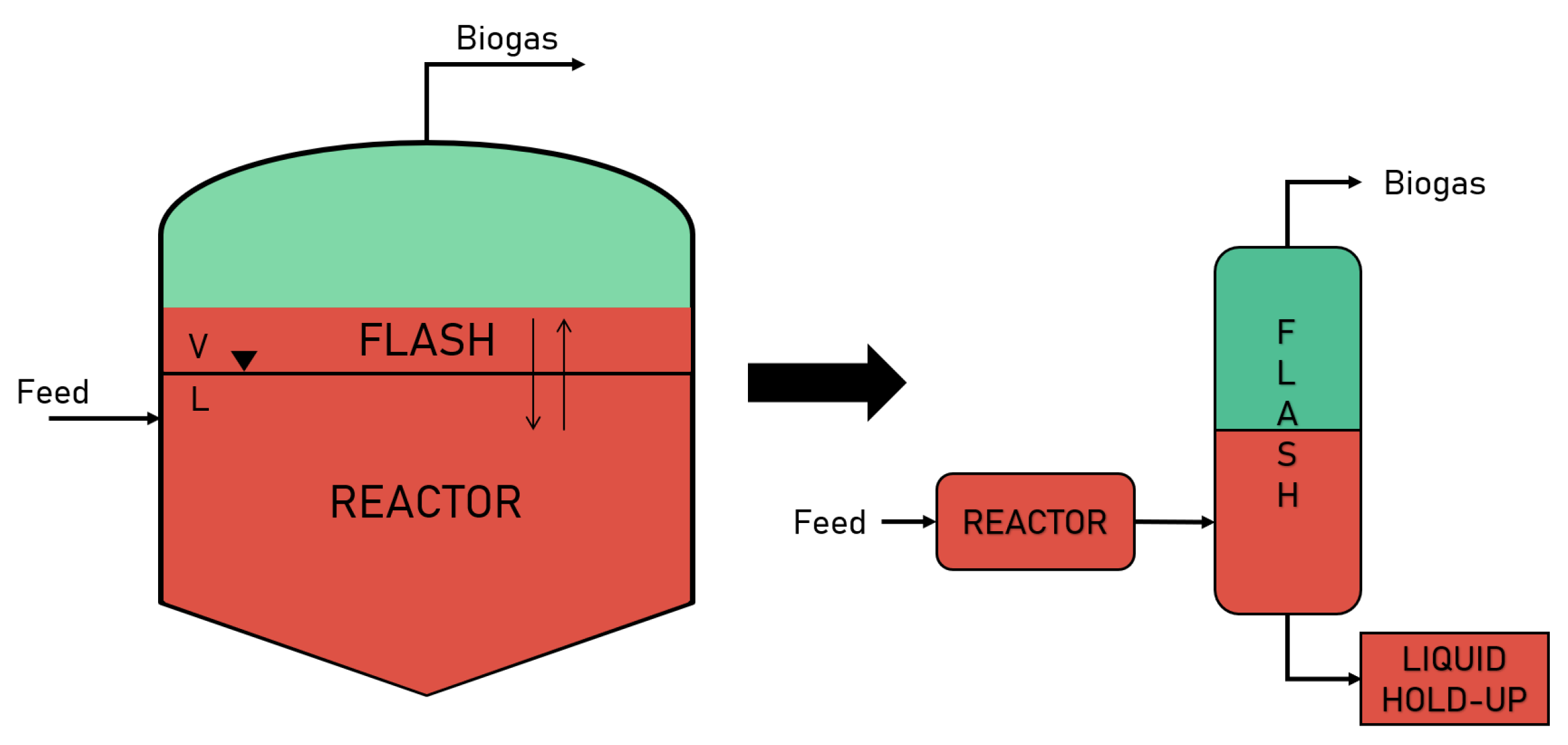
2.1. Model Assumptions and Schematisation

The species in the anaerobic system whose thermodynamic properties and interactions have been studied are $\mathrm{C}{\mathrm{H}}_4$, $\mathrm{C}{\mathrm{O}}_2$, ${\mathrm{H}}_2\mathrm{S}$ and ${\mathrm{H}}_2\mathrm{O}$. The liquid phase of a digester can be easily treated as a homogeneous continuous stirred tank reactor [12], where all the bio reactions take place. Particulate substances enter the reactor with a certain load and concentration, degrade and produce, mainly, methane, carbon dioxide and hydrogen sulphide. Hydrogen production is not taken into consideration since its production is very small (∼ppm) due to syntrophic interactions [13], and will not be accounted in later calculations.

The volatility of these elements is high enough to move them from aqueous phase toward into gas phase. As bubbles, these species exit the liquid free surface of the digester towards the headspace, where are collected and sent in post-processing units. At this point, it is possible to see the phase-changing phenomena and the crossing of the liquid free surface in analogy with a flash process, where vapour–liquid equilibrium (VLE) is established. An effective schematisation of this process is reported in Figure 1.

At equilibrium conditions (i.e., steady-states), the production of biogas has reached its steady conditions. Consequently, it is possible to assume that the biogas composition remains the same for a certain period of time (this assumption decays when important variations happens on the organic loading rate or in the feedstock loading conditions, that subsequently change the biomass reactivity). Thus, no reactions take place in the flash unit.

Moreover, it is assumed to be an isothermal and adiabatic unit, since the AD works mostly at the same temperature, established by weather conditions and biomass stability [14]. The adiabatic assumption simplifies the equilibrium study, being the heat transfer phenomena not the objective of this work.

Similar to a semi-batch reactor, an AD unit releases biogas constantly from the top while the liquid phase remains in the reactor vessel until all biomass is consumed or cleaning processes are required. In order to take into account this feature of the reactor, the flash outlet liquid is modelled so that the liquid stream enters a fictitious unit (i.e., liquid hold-up).

2.2. Multi-Parameter Helmholtz-Energy Equations of State

The availability of highly accurate thermophysical property data is crucial for the design and optimisation of many industrial applications, such as the AD process covered in this research.

The achievement of such goal, which is essential from the economic point of view, but also from the point of view of safety and sustainability, surely requires extremely precise thermodynamic modelling. The most efficient and widely used approach in this kind of studies is represented by Helmholtz EoS. Indeed, these multi-parameter EoS allow to derive the thermodynamic properties of gases and liquids with high accuracy, as highlighted in several literature works [15,16,17].

Based on these considerations, the Helmholtz EoS model has been adopted in order to describe the thermodynamic behaviour of the mixtures of interest within research purpose. In particular, different fundamental EoS for pure fluids have been selected after a published literature search and implemented in a Python algorithm. The substances considered in this work, as mentioned in Section 2.1, are mainly: methane [18], carbon dioxide [19], hydrogen sulfide [15] and water [20]. However, also carbon monoxide [15], oxygen [21], hydrogen [22], ammonia [23], ethanol [24], methanol [25] and ethylene [26] have been taken into account, both because these chemical constituents are often present in the AD’s products and because it was decided to devise a code that it was as versatile as possible. The depiction of these compounds can be found directly in the source code (Section 2.6).

We have focused only on pure substances for the sake of simplicity and to improve the algorithm’s computation time, but EoS written in terms of the Helmholtz energy has been developed also for mixtures [27,28].

In general, the reduced Helmholtz energy function $\alpha$ is commonly split into two terms:

$$\alpha \left(\delta ,\tau \right)=\frac{a\left(\rho ,T\right)}{\mathrm{R}T}={\alpha }^{\mathrm{o}}\left(\delta ,\tau \right)+{\alpha }^{\mathrm{r}}\left(\delta ,\tau \right)$$

(1)

where $a\left(\rho ,T\right)$ is the molar Helmholtz energy, $\delta =\rho /{\rho }_{\mathrm{c}}$ is the reduced density, $\tau =T_{\mathrm{c}}/T$ is the inverse reduced temperature (with the critical-point parameters used as the reducing density and reducing temperature) and ${\alpha }^{\mathrm{o}}$ and ${\alpha }^{\mathrm{r}}$ respectively represent the ideal gas contribution to the Helmholtz free energy and the residual fluid behaviour:

$${\alpha }^{\mathrm{o}}\left(\delta ,\tau \right)=ln\left(\delta \right)+a_1^{\mathrm{o}}+a_2^{\mathrm{o}}\tau +a_3^{\mathrm{o}}ln\left(\tau \right)+\sum _j{a}_j^{\mathrm{o}}ln\left[1-exp\left(-\tau {\theta }_j^{\mathrm{o}}\right)\right]$$

(2)

$$\begin{array}{cc}\hfill {\alpha }^{\mathrm{r}}\left(\delta ,\tau \right)=& \sum _j{n}_j{\delta }^{d_j}{\tau }^{t_j}+\sum _j{n}_j{\delta }^{d_j}{\tau }^{t_j}{e}^{-{\delta }^{{\mathrm{C}}_j}}+\sum _j{n}_j{\delta }^{d_j}{\tau }^{t_j}{e}^{-{\alpha }_j{\left(\delta -{\epsilon }_j\right)}^2-{\beta }_j{\left(\tau -{\gamma }_j\right)}^2}\hfill \\ \hfill & +\sum _j{n}_j{\Delta }^{b_j}\delta e^{-{\mathrm{C}}_j{\left(\delta -1\right)}^2-D_j{\left(\tau -1\right)}^2}\hfill \end{array}$$

(3)

As mentioned above, all thermodynamic properties of a substance can be calculated from Equation (1) and its derivatives with respect to the independent variables on which the equation depends. Some of these useful relations are summarised below:

• Density: it is obtained by solving the following equation

  $$P=-\frac{\partial a}{\partial v}$$

  (4)
• Entropy:

  $$s=-\frac{\partial a}{\partial T}$$

  (5)
• Enthalpy:

  $$h=A-T\frac{\partial a}{\partial T}-v\frac{\partial a}{\partial v}$$

  (6)
• Fugacity coefficient:

  $$ln\varphi ={\int }_0^P\left[\frac{v\left(T,P\right)}{\mathrm{R}T}-\frac{1}{P}\right]\mathrm{d}P$$

  (7)

More details on this topic and, more generally, on the structure of Helmholtz’s equations and its derivatives are given in the work of Span [29].

2.3. Density Algorithm

One of the main issues experienced using Equation (1) for flash calculations concerns the density estimation. Indeed, the variables needed to evaluate the VLE inside the reactor are P, T and the feed composition z, whereas Helmholtz functions depend on $\rho$ and T. Hence, with temperature and pressure given, the nonlinear Equation (8), derived by Equation (4), needs to be solved numerically.

$$P=\rho R_{\mathrm{spec}}T\left(1+\delta \frac{\partial {\alpha }^{\mathrm{r}}}{\partial \delta }\right)$$

(8)

The routine to figure out this problem is a key element in flash calculations, since various solutions could be found and since it is particularly important to check that the proper density is estimated. Indeed, these thermodynamic models can have multiple loops in the two phase region generating more than the cubic EoS’ three roots for $\rho$ and where only the outermost solutions are to be considered (see Figure 2a,c for an example of the complex behaviour of $P\left(\rho \right)$ function, evaluated at different temperatures, for carbon dioxide and hydrogen sulfide, respectively). An advanced and worthwhile procedure to work out this issue has been described by Gernert et al. (2014) [30]. However, a simplified approach to this method has been adopted in this project.

First of all, the function in Equation (8) has been studied for each substance in order to find the proper guess value for each phase (the results provided by this analysis, carried out at different temperatures, are plotted in Figure 2). As pointed out by Gernert et al. (2014) [30], the solution to the left of the first maximum of the isotherm in $P-\rho$ diagram corresponds to the vapour density, while the one to the right of the last minimum is the liquid density. For this reason, initial estimates close to the values mentioned above have been chosen and used to solve numerically the density equation. It is interesting to note that, at fixed pressure, for temperatures higher than the critical one, the isotherms show only one density root (as the case concerning $\mathrm{C}{\mathrm{H}}_4$, displayed in Figure 2b).

When this analysis is applied to substances with a boiling point above the considered temperature range, as in the case of water, Equation (8) returns peculiar results. Indeed, as shown in Figure 2d, there is no maximum at low $\rho$ values, but only extremely steep curves at high densities. The behavior of the $P\left(\rho \right)$ function is physically correct (and this proves the consistency and the validity of the adopted model) because water, at these temperatures, is mainly in the liquid phase and thus no vapour density root exists. Therefore, we focused exclusively on the liquid density range and we have selected the same guess value for both phases.

2.4. Rachford–Rice Algorithm

Once the density problem is fixed, the VLE can be computed through the flash resolution algorithm explained briefly below.

First of all, given T and P, the k-values can be estimated using the following formula:

$$ln{k}_i=ln\frac{y_i}{x_i}=ln\frac{{\widehat{\varphi }}_i^{\ell }}{{\widehat{\varphi }}_i^{\mathrm{v}}}$$

(9)

where ${\widehat{\varphi }}_i^{\ell }$ and ${\widehat{\varphi }}_i^{\mathrm{v}}$ are derived using the procedure described in Section 2.5. The relation (9) is then used to evaluate the Rachford–Rice equation [31]

$$f\left(\gamma \right)=\sum _{i=1}^N\frac{z_i\left(k_i-1\right)}{1+\gamma \left(k_i-1\right)}=0$$

(10)

with $\gamma$ vapour fraction. The resolution of Equation (10) allows to calculate the phase compositions through these expressions

$$x_i=\frac{z_i}{1+\gamma \left(k_i-1\right)}$$

(11)

$$y_i=\frac{z_i{k}_i}{1+\gamma \left(k_i-1\right)}$$

(12)

To have a reliable evaluation of the liquid and vapour fraction exiting the unit, a precise calculation of the mixture fugacities is needed. Since they are dependent from the compositions, an iterative procedure is established:

• $x,y$ are set, as first guess, equal to the inlet composition.
• The value of the k is obtained through Equation (9) and used in the VLE solution.
• $x,y$ are updated through Equations (11) and (12).
• New values for ${\widehat{\varphi }}_i^{\ell ,\mathrm{v}}$ are updated following the procedure in Section 2.5.
• Iterate from point 2.

This operation, implemented to increase the accuracy of the measurements [32], is repeated until $x_{i,j}\simeq x_{i,j+1}$ and $y_{i,j}\simeq y_{i,j+1}$ (the index j denotes the j-th step in the iteration process). Numerically speaking, this process is iterated until the absolute differences of these quantities $\Delta x,\Delta y$ are less or equal to a fixed threshold $\epsilon$, set to $1\times {10}^{-5}$ to reach the highest precision possible. Refer to Figure 3 for a visual representation of the algorithm described above.

2.5. Fugacity of Mixture Evaluation

As stated in Section 2.2, there are a lot of variants of the Helmholtz EoS for the evaluation of the mixing properties from a binary mixtures [33], and a generalised form can be found in the work of Lemmon and Tillner-Roth (1999) [27]. However, no advances are present for bigger mixtures, with three or four components. Being the case of this work, to evaluate the fugacity of the species in the mixture of the four components taken under consideration ($\mathrm{C}{\mathrm{H}}_4$, $\mathrm{C}{\mathrm{O}}_2$, ${\mathrm{H}}_2\mathrm{S}$ and ${\mathrm{H}}_2\mathrm{O}$), a hybrid approach was developed.

The compressibility factor (Z) of the mixture in that conditions is evaluated using a specific relation of the reduced free-Helmholtz energy and reduced density (Equation (13)), while the fugacity of the mixture for a specific species i is evaluated from the Peng–Robinson cubic expression [34,35], as in Equation (14)

$$Z=1+\delta {\left(\frac{\partial {\alpha }^{\mathrm{r}}}{\partial \delta }\right)}_{\tau }$$

(13)

$$ln{\widehat{\varphi }}_i=\frac{B_i}{B}(Z-1)+\frac{A}{2\sqrt{2}B}\left(\frac{B_i}{B}-2\sqrt{\frac{A_i}{A}}\right)ln\left(\frac{Z+B(1+\sqrt{2})}{Z+B(1-\sqrt{2})}\right)-ln(Z-B)$$

(14)

where A and B are specific thermodynamic parameters of the Peng–Robinson EoS, and $A_i$ and $B_i$ are the same properties evaluated with mixing rules. For these parameters and relative derivations please refer to the official literature [36]. The procedure for $\widehat{{\varphi }_i}$ evaluation is the following:

• Define the process operative conditions (temperature and pressure).
• Evaluate the density of the mixture at that conditions with Equation (8).
• Evaluate from Equation (13) the Z of the mixture at defined temperature and pressure.
• Evaluate all the thermodynamic parameters A, B, $A_i$ and $B_i$.
• Evaluate the fugacity of the mixture with the Z got at the previous point with Equation (14).

It has been noticed that the acquired results through this approach, as well as for the evaluation on the Z, are significantly more stable and coherent rather than using a cubic EoS (i.e., Peng–Robinson). This is a further confirmation on the reliability and robustness of the EoS chosen for that study.

2.6. Calculation Tool

This study has been developed with the programming language Python™. The scripts can be found on the relative GitHub page, and all the packages required to compile them are listed in the requirements file.

3. Results

The data used in simulations and comparisons performed in this section come from the industrial scene, in particular from a northern Italian company, namely, Th$\ddot{\mathrm{o}}$ni s.r.l., which provided us the biogas composition and the total amount of water in the reactor. From these it is possible to retrieve all the necessary information to properly run a simulation. These data are shown in

Table 2. Data about inlet composition and reactor load, shared by industrial company, already converted and ready-to-use for simulation.

Name	Value	Units
Feed flowrate 1	100	$\mathrm{kmol}/\mathrm{d}$
$z_{\mathrm{C}{\mathrm{H}}_4}$	0.0067	–
$z_{\mathrm{C}{\mathrm{O}}_2}$	0.0022	–
$z_{{\mathrm{H}}_2\mathrm{S}}$	0.0001	–
$z_{{\mathrm{H}}_2\mathrm{O}}$2	0.9911	–

¹ Feed flowrate can be considered as both an actual flow entering the reactor, expressed as in table or a daily load of feedstock, independent from time. ² Compositions of biogas species are reported in wet basis.

.

3.1. Hybrid Approach vs. Cubic-Based Mixture Fugacity

As stated in the previous section, during the analysis, it has been noticed that the fugacity of the mixture evaluated with the new procedure (Equations (13) and (14)) is much more reliable than that evaluated only with the cubic one. The results of the comparison, between the hybrid approach and the PR calculation, are shown in

Table 3. Results comparison between the mixture fugacity evaluated with the PR and with the hybrid approach.

Species	${\mathit{Z}}_{\mathbf{PR}}$	${\mathit{Z}}_{\mathbf{Hybrid}}$	${\widehat{\mathit{\varphi }}}_{\mathbf{PR}}$	${\widehat{\mathit{\varphi }}}_{\mathbf{Hybrid}}$
$\mathrm{C}{\mathrm{H}}_4$	$9.64\times {10}^{-8}$	1.006	$1.07\times {10}^9$	0.9997
$\mathrm{C}{\mathrm{O}}_2$	$9.33\times {10}^{-8}$	1.010	$1.26\times {10}^{-3}$	0.9946
${\mathrm{H}}_2\mathrm{S}$	$9.38\times {10}^{-8}$	1.014	$6.11\times {10}^{-4}$	0.9895
${\mathrm{H}}_2\mathrm{O}$	–	1.023	–	0.9435

. The calculation has been performed considering mesophilic condition (35 °C, 1 atm).

In both cases, the fugacity is evaluated with Equation (14). Being the operating conditions the same for both cases, the value of this parameter is strictly dependent on the value of the compressibility factor Z. In the case of the cubic EoS, Z is evaluated analytically as the root of the third grade characteristic polynomial with Cardano’s method. However, the values obtained with this method stick around $9\times {10}^{-8}$, revealing a lack of sensibility and precision when, in the wet system, low values of gas composition are present (i.e., water amount > 97 %wt.). The resulting fugacity values are on the same trend, revealing a strong non ideality of the gaseous mixture. On the other hand, the compressibility factor found through Equation (13) has more reasonable and reliable values. In fact, the Z and $\widehat{\varphi }$ values for $\mathrm{C}{\mathrm{H}}_4$ suggest an almost-ideal behavior, that can be linked to the low amount of methane which solely dissolves in the liquid phase [37], thus going in the gas phase accumulating in headspace. The $\mathrm{C}{\mathrm{O}}_2$ on the contrary has a good solubilisation in water in these conditions. Thus, its shifting between these two states (gas and liquid) makes it deviate more from ideal conditions, increasing Z and decreasing $\widehat{\varphi }$ values. In the same way, the ${\mathrm{H}}_2\mathrm{S}$ not only has a good water solubilisation, but, due to its low amount produced in the liquid phase, the Z and $\widehat{\varphi }$ values highlight its heavier deviation from the ideal. Greatly interesting are the results from ${\mathrm{H}}_2\mathrm{O}$ analysis. Due to the operating conditions considered, it is impossible to find the root for the cubic EoS, and so, no mixture fugacity was found, since all the water in this condition is completely liquid (besides the amount volatilised respecting equilibrium). On the other hand, the Helmholtz EoS has been capable to efficiently calculate both the Z and the relative fugacity in this complex condition, showing a stronger non-ideal behavior with respect to the other ones.

3.2. Temperature and Pressure Optimisation

The vapour–liquid equilibrium is strongly affected by the operating conditions of the units, namely, pressure and temperature levels. To better understand these behaviours, different simulations were done at different temperature and pressures. These are chosen accordingly to the physics of the system: temperature values range between 20 and 55 °C, increased by 5 °C every simulation, while pressure values are 0.3 atm, 0.5 atm, 1 atm and 1.5 atm, in order to keep track of the system in vacuum, light vacuum, ambient (nominal) and high pressure conditions, respectively. Therefore, a total number of 32 simulations were performed, obtaining 32 resulting points. These are shown in the following figures.

As it is possible to see from Figure 4a, the vapour fraction increases with temperature but decreases with pressure. At 1 atm, the trend is approximable to a linear increase. With increase in pressure, toward 1.5 atm, the trend becomes similar to a logarithmic one. On the other hand, while decreasing in pressure, the trend assumes an exponential shape with respect to temperature. This is understandable since the lower the pressure, the higher the extent of the species to pass from liquid to gaseous phase. This behaviour is then reflected in the trends of both exiting liquid and vapour molar flows.

The trend of the vapour fraction (Figure 4b) is highly similar to the one of $\gamma$, and the liquid trend (Figure 4c) is mirror to them. The high amount of liquid flow resembles the high content of water in the liquid phase. Obviously, the absolute amount of vapour produced is much less with respect to the liquid one due to inlet load of water. Consequently, it is rather trivial that to maximise vapour (in particular, biogas) production, the pressure should be the lowest possible and the temperature the highest one. However, these conditions can damage the microorganism metabolism and strongly hinder the dynamic global production [38].

Looking at the graphs showing the compositions of the outlet liquid phase (Figure 5), it is possible to notice intriguing trends. Firstly, the amount of total volatile component produced decreases with the increase of temperature and reduction of pressure, as it should be. However, it is possible to find noticeably quantity of methane in water (Figure 5a) with respect to carbon dioxide (Figure 5b), despite the latter being much more soluble than the former. This is because the absolute amount of methane produced is much higher than other volatile elements.

Furthermore, the trend of the gaseous fraction with respect to pressure, depicted in Figure 6, is of interest. The gaseous $\mathrm{C}{\mathrm{H}}_4$ and $\mathrm{C}{\mathrm{O}}_2$ fractions both decrease with the increase in temperature. This happens because the absolute amount of water which is volatilising is much higher than the other species.

This trend can be also explained looking at the relative volatility of these components (Figure 6e) with respect to water. This quantity has been evaluated through the ratio between the vapour pressure of the species with respect to water. Interestingly, the volatilities decrease with the increase in temperature. This behavior can be only explained by looking at the vapour pressure rate of change (Figure 6f). This quantity is evaluated as the change of the vapour pressure value with respect to the temperature variation, as reported in Equation (15):

$$\frac{\mathrm{d}{P}_{\mathrm{sat}}\left(T\right)}{\mathrm{d}T}=\frac{P_{\mathrm{sat}}\left(T_i\right)-P_{\mathrm{sat}}\left(T_{i-1}\right)}{T_i-T_{i-1}}$$

(15)

where $T_i$ corresponds to a specific temperature element in the array of temperatures considered.

These trends are normalised using the max value for every species. The light-key components have a steeper slope with respect to ${\mathrm{H}}_2\mathrm{O}$ until the temperature becomes 35 °C. At this point, the slopes of these components become lower than the ${\mathrm{H}}_2\mathrm{O}$ one. Consequently, the absolute amount of water released in the vapour phase becomes significant, justifying its exponential increase.

This also explains the max values reached at this temperature for the $\mathrm{C}{\mathrm{O}}_2$ at 1 and 1.5 atm, and the ${\mathrm{H}}_2\mathrm{S}$ at 0.3 atm (Figure 6b–d). $\mathrm{C}{\mathrm{H}}_4$ has a monotonic trend at every temperature and pressure, and at 35 °C and 1.5 atm the curve has an inflection point: at lower T, the amount of methane released is analogue to the amount of the $\mathrm{C}{\mathrm{H}}_4$ released in vacuum conditions; at higher temperature, the methane fraction increases, reaching the highest value at 50 °C. From Figure 6a it is possible to understand that the highest amount of methane is achieved at lower temperature and ambient pressure, specifically 30–35 °C and 1 atm. Moreover, lower ${\mathrm{H}}_2\mathrm{S}$ and ${\mathrm{H}}_2\mathrm{O}$ content are achieved, making these the proper working conditions. On the contrary, the $\mathrm{C}{\mathrm{O}}_2$ produced reaches the maximum for that temperature at ambient pressure, but the purity of the methane justifies the results.

On the other hand, if the purpose is the lowest production possible of $\mathrm{C}{\mathrm{O}}_2$, working at the same temperature range at lower pressure reveals a good trade-off concerning the biogas purity. From the transport phenomena point of view, temperature and pressure not only influence the amount of biogas produced and its thermodynamics, but also the mechanism and extent with which these volatile components pass from a liquid to a vapour phase.

In Figure 7, both the absolute and normalised values of the molar fluxes for every species at each temperature and pressure are reported. The latter are normalised by the max value of the array, achieved at a specific condition.

To evaluate these quantities, the diffusion of a species from the liquid to the upper gas phase was considered (Figure 8). The species diffuse due to the concentration gradient across the interface. However, its evaluation is not trivial: the partial pressure gradient in the vapour phase has been considered, taking into account also its relative humidity, making the calculation of the molar flow and concentration profile faster and more reliable.

Because there are very few volatile species in the unit, it is assumed that the liquid is a stagnant system (i.e., the momentum impressed by the mixing motor is negligible), and that they do not interact with each other but only with the continuous aqueous phase. So, three binary non-reacting systems were studied, namely, $\mathrm{C}{\mathrm{H}}_4$-${\mathrm{H}}_2\mathrm{O}$, $\mathrm{C}{\mathrm{O}}_2$-${\mathrm{H}}_2\mathrm{O}$ and ${\mathrm{H}}_2\mathrm{S}$-${\mathrm{H}}_2\mathrm{O}$. Starting from the second Fick’s law [39,40], the specific molar flow of a general species has been developed (Equation (16)).

$${\mathrm{J}}_i(T,P)=\frac{P{\mathcal{D}}_{i,{\mathrm{H}}_2\mathrm{O}}}{\mathrm{R}T\mathrm{L}}\ln \left(\frac{P-\psi P_{\mathrm{sat},i}\left(T\right)}{P-P_{\mathrm{sat},i}\left(T\right)}\right)$$

(16)

The diffusion coefficients of the species into water were found in accordance with the works of Moradi et al. (2020) [41] for $\mathrm{C}{\mathrm{H}}_4$, Tamimi et al. (1994) [42] for $\mathrm{C}{\mathrm{O}}_2$ and ${\mathrm{H}}_2\mathrm{S}$, and Haimour and Sandall (1984) [43] for ${\mathrm{H}}_2\mathrm{S}$. The relations found were used to evaluate the diffusion coefficients according to the operative conditions and unit properties under study (see

Table 4. Comparison between diffusivities found in the literature and predictions provided by this work.

	${\mathcal{D}}_{\mathbf{CH}{}_4,\mathbf{H}{}_2\mathbf{O}}\left[{\mathbf{m}}^2/\mathbf{s}\right]·{10}^{-9}$
T[K]	This work	Literature
298.15	1.86	1.88
308.15	2.16	2.12
318.15	2.38	2.41
328.15	2.75	–
	${\mathcal{D}}_{\mathbf{CO}{}_2,\mathbf{H}{}_2\mathbf{O}}\left[{\mathbf{m}}^2/\mathbf{s}\right]·{10}^{-9}$
T[K]	This work	Literature
298.15	2.29	2.11
308.15	2.96	2.73
318.15	3.72	3.43
328.15	4.58	4.22
	${\mathcal{D}}_{\mathbf{H}{}_2\mathbf{S},\mathbf{H}{}_2\mathbf{O}}\left[{\mathbf{m}}^2/\mathbf{s}\right]·{10}^{-9}$
T[K]	This work	Literature
298.15	1.03	1.87
308.15	1.25	2.47
318.15	1.48	–
328.15	1.74	–

).

From Equation (16), it is also possible to derive the partial pressure profile along the gaseous phase. A visual representation of it is present in Figure 8, where, while the liquid phase concentration remains the same, the gas concentration decreases, moving away from the liquid free surface, having the minima on the top of the headspace. Obviously, this process is part of the dynamic of the reactor and has not been considered, since, at steady-state conditions, the profile resembles a straight line coincident to that of the liquid phase.

The dimension of the reactor, as height, liquid level and diameter, has been provided by the company. As said, the reaction contribution was not considered due to the assumption made. This brings us to a higher molar flux for the $\mathrm{C}{\mathrm{O}}_2$ with respect to $\mathrm{C}{\mathrm{H}}_4$, as shown in the figure.

As it is possible to see, working at mid-higher pressure ensures a higher absolute gas productivity. However, high ${\mathrm{H}}_2\mathrm{S}$ content is achieved with respect to the other gases. A trade-off is necessary between the ambient and high pressure. Both $\mathrm{C}{\mathrm{H}}_4$ and ${\mathrm{H}}_2\mathrm{S}$ have a max trend, while $\mathrm{C}{\mathrm{O}}_2$ is monotonically increasing with temperature and pressure. As far as $\mathrm{C}{\mathrm{H}}_4$ is concerned, both 30 °C and 35 °C resemble a maximum point. The former is reached at 0.5 atm, while the latter is reached for higher pressure conditions. This goes in accordance with the thermodynamic analysis previously done.

On the other hand, it is possible to see that working at higher temperature means decrease the purity of the biogas. Upon reaching 45 °C, at every pressure value, a peak of ${\mathrm{H}}_2\mathrm{S}$ is achieved. Despite the low relative amount, it is always suggested to avoid these conditions.

4. Conclusions

This work aims to bring new advances in the anaerobic digestion field. A thermodynamic study of an industrial reactor has been done to assess how the productivity of the unit, at different operative conditions, will be affected. From this point of view, it has been seen that, working in the range of mesophilic conditions (30 °C–35 °C) at slightly higher pressure than atmospheric (i.e., in the range of 1 atm to 1.5 atm), it is possible to optimise the biogas purity, reducing the relative content of other products such as $\mathrm{C}{\mathrm{O}}_2$ and ${\mathrm{H}}_2\mathrm{S}$. Interestingly, it has been demonstrated that a significant amount of water vapourises into the gas phase due to equilibrium conditions (about 5 %wt.), a non-negligible amount for further treatments and evaluation. Many industrial processes work at slight thermophilic conditions (about 42 °C–45 °C); however, from the analysis previously reported, it is not convenient since a larger amount of ${\mathrm{H}}_2\mathrm{S}$ (about 20% more) goes into the exiting biogas, reducing the methane content and increasing the post-treatment costs.

References

1. Scarlat, N.; Fahl, F.; Dallemand, J.F.; Monforti, F.; Motola, V. A spatial analysis of biogas potential from manure in Europe. Renew. Sustain. Energy Rev. 2018, 94, 915–930. [Google Scholar] [CrossRef]
2. Muhayodin, F.; Fritze, A.; Rotter, V.S. Mass balance of C, nutrients, and mineralization of nitrogen during anaerobic co-digestion of rice straw with cow manure. Sustainability 2021, 13, 11568. [Google Scholar] [CrossRef]
3. Achinas, S.; Li, Y.; Achinas, V.; Euverink, G.J.W. Biogas potential from the anaerobic digestion of potato peels: Process performance and kinetics evaluation. Energies 2019, 12, 2311. [Google Scholar] [CrossRef] [Green Version]
4. Anukam, A.; Mohammadi, A.; Naqvi, M.; Granström, K. A review of the chemistry of anaerobic digestion: Methods of accelerating and optimizing process efficiency. Processes 2019, 7, 504. [Google Scholar] [CrossRef] [Green Version]
5. Wang, X.; Cheng, S.; Li, Z.; Men, Y.; Wu, J. Impacts of cellulase and amylase on enzymatic hydrolysis and methane production in the anaerobic digestion of corn straw. Sustainability 2020, 12, 5453. [Google Scholar] [CrossRef]
6. Kamperidou, V.; Terzopoulou, P. Anaerobic digestion of lignocellulosic waste materials. Sustainability 2021, 13, 12810. [Google Scholar] [CrossRef]
7. Bajpai, P. Anaerobic Technology in Pulp and Paper Industry; Springer Briefs in Applied Sciences and Technology; Springer: Berlin/Heidelberg, Germany, 2017. [Google Scholar]
8. Chen, W.S.; Strik, D.P.B.T.B.; Buisman, C.J.N.; Kroeze, C. Production of Caproic Acid from Mixed Organic Waste: An Environmental Life Cycle Perspective. Environ. Sci. Technol. 2017, 51, 7159–7168. [Google Scholar] [CrossRef] [Green Version]
9. Bühlmann, C.H.; Mickan, B.S.; Tait, S.; Renton, M.; Bahri, P.A. Lactic acid from mixed food wastes at a commercial biogas facility: Effect of feedstock and process conditions. J. Clean. Prod. 2021, 284, 125243. [Google Scholar] [CrossRef]
10. Wasajjaa, H.; Lindeboom, R.E.F.; van Lier, J.B.; Aravind, P.V. Techno-economic review of biogas cleaning technologies for small scale off-grid solid oxide fuel cell applications. Fuel Process. Technol. 2020, 197, 106215. [Google Scholar] [CrossRef]
11. Muvhiiwa, R.F.; Hildebrandt, D.; Glasser, D.; Matambo, T. A Thermodynamic Approach Toward Defining the Limits of Biogas Production. AIChE J. 2015, 61, 4270–4276. [Google Scholar] [CrossRef]
12. Batstone, D.; Keller, J.; Angelidaki, I.; Kalyuzhnyi, S.; Pavlostathis, S.; Rozzi, A.; Sanders, W.; Siegrist, H.; Vavilin, V. Anaerobic digestion model No 1 (ADM1). Water Sci. Technol. A J. Int. Assoc. Water Pollut. Res. 2002, 45, 65–73. [Google Scholar] [CrossRef]
13. Zappi, A.; Hernandez, R.; Holmes, W. A review of hydrogen production from anaerobic digestion. Int. J. Environ. Sci. Technol. 2021, 18, 4075–4090. [Google Scholar] [CrossRef]
14. Carotenuto, C.; Guarino, G.; Minale, M.; Morrone, B. Biogas Production from Anaerobic Digestion of Manure at Different Operative Conditions. Intern. J. Heat Tech. 2016, 34, 623–629. [Google Scholar] [CrossRef]
15. Lemmon, E.W.; Span, J. Short Fundamental Equations of State for 20 Industrial Fluids. Chem. Eng. Data 2006, 51, 785–850. [Google Scholar] [CrossRef]
16. Wilhelmsen, Ø.; Aasen, A.; Skaugen, G.; Aursand, P.; Austegard, A.; Aursand, E.; Gjennestad, M.A.; Lund, H.; Linga, G. Hammer, M. Thermodynamic Modeling with Equations of State: Present Challenges with Established Methods. Ind. Eng. Chem. Res. 2017, 56, 3503–3515. [Google Scholar] [CrossRef] [Green Version]
17. Herrig, S. New Helmholtz-Energy Equations of State for Pure Fluids and CCS-Relevant Mixtures. Ph.D. Thesis, Ruhr-Universität Bochum, Bochum, Germany, 2018. [Google Scholar]
18. Setzmann, U.; Wagner, W. A New Equation of State and Tables of Thermodynamic Properties for Methane Covering the Range from the Melting Line to 625 K at Pressures up to 1000 MPa. J. Phys. Chem. Ref. Data 1991, 20, 1061–1155. [Google Scholar] [CrossRef] [Green Version]
19. Span, R.; Wagner, W. A New Equation of State for Carbon Dioxide Covering the Fluid Region from the Triple-Point Temperature to 1100 K at Pressures up to 800 MPa. J. Phys. Chem. Ref. Data 1996, 25, 1509–1596. [Google Scholar] [CrossRef] [Green Version]
20. Wagner, W.; Pruß, A. The IAWPS Formulation 1995 for the Thermodynamic Properties of Ordinary Water Substance for General and Scientific Use. J. Phys. Chem. Ref. Data 2002, 31, 387–535. [Google Scholar] [CrossRef] [Green Version]
21. Schmidt, R.; Wagner, W. A New Form of the Equation of State for Pure Substances and Its Application to Oxygen. Fluid Phase Equilibria 1985, 19, 175–200. [Google Scholar] [CrossRef]
22. Leachman, J.W.; Jacobsen, R.T.; Penoncello, S.G.; Lemmon, E.W. Fundamental Equations of State for Parahydrogen, Normal Hydrogen, and Orthohydrogen. J. Phys. Chem. Ref. Data 2009, 38, 721. [Google Scholar] [CrossRef]
23. Baehr, H.D.; Tillner-Roth, R. Thermodynamische Eigenschaften umweltverträglicher Kältemittel/Thermodynamic Properties of Environmentally Acceptable Refrigerants: Zustandsgleichungen und Tafeln für Ammoniak, R 22, R 134a, R 152a und R 123/Equations of State and Tables for Ammonia, R 22, R 134a, R 152a and R 123, 1st ed.; Springer: Heidelberg, Germany, 1995. [Google Scholar] [CrossRef]
24. Schroeder, J.A.; Penoncello, S.G.; Schroeder, J.S. A Fundamental Equation of State for Ethanol. J. Phys. Chem. Ref. Data 2014, 43, 4. [Google Scholar] [CrossRef]
25. Kume, D.; Sakoda, N.; Uematsu, M. An Equation of State for Thermodynamic Properties for Methanol. J. Chem. Eng. Data 2005, 28, 2. [Google Scholar]
26. Smukala, J.; Span, R.; Wagner, W. New Equation of State for Ethylene Covering the Fluid Region for Temperatures From the Melting Line to 450 K at Pressures up to 300 MPa. J. Phys. Chem. Ref. Data 2000, 29, 1053–1121. [Google Scholar] [CrossRef]
27. Lemmon, E.W.; Tillner-Roth, R. A Helmholtz Energy Equation of State for Calculating the Thermodynamic Properties of Fluid Mixtures. Fluid Phase Equilibria 1999, 165, 1–21. [Google Scholar] [CrossRef]
28. Kunz, O.; Wagner, W. The GERG-2008 wide-range equation of state for natural gases and other mixtures: An expansion of GERG-2004. J. Chem. Eng. Data 2012, 57, 3032–3091. [Google Scholar] [CrossRef]
29. Span, R. Multiparameter Equations of State: An Accurate Source of Thermodynamic Property Data, 1st ed.; Springer: Berlin, Germany, 2000. [Google Scholar]
30. Gernert, J.; Jäger, A.; Span, R. Calculation of phase equilibria for multi-component mixtures using highly accurate Helmholtz energy equations of state. Fluid Phase Equilibria 2014, 375, 209–218. [Google Scholar] [CrossRef]
31. Rachford, H.H.; Rice, J.D. Procedure for use of electronic digital computers incalculating flash vaporization hydrocarbon equilibrium. J. Petrol. Technol. 1952, 24, 19. [Google Scholar] [CrossRef]
32. Prausnitz, J.; Chueh, P. Computer Calculations for High-Pressure Vapor–LiquidEquilibria; Prentice-Hall: Englewood Cliffs, NJ, USA, 1968. [Google Scholar]
33. Tillner-Roth, R.; Friend, D.G. A Helmholtz Free Energy Formulation of the Thermodynamic Properties of the Mixture Water + Ammonia. J. Phys. Chem. Ref. Data 1998, 27, 63–96. [Google Scholar] [CrossRef] [Green Version]
34. Mathias, P.M.; Copeman, W.T. Extension of the Peng-Robinson equation of state to complex mixtures: Evaluation of the various forms of the local composition concept. Fluid Phase Equilibria 1983, 13, 91–108. [Google Scholar] [CrossRef]
35. Lin, C.; Daubert, E.T. Estimation of Partial Molar Volume and Fugacity Coefficient of Components in Mixtures from the Soave and Peng-Robinson Equations of State. Ind. Eng. Chem. Process Des. Dev. 1980, 19, 51–59. [Google Scholar] [CrossRef]
36. Peng, D.; Robinson, B.D. A New Two-Constant Equation of State. Ind. Eng. Chem. Fundamen. 1976, 15, 59–64. [Google Scholar] [CrossRef]
37. Frost, M.; Karakatsani, E.; von Solms, N.M.; Richon, D.; Kontogeorgis, G.M. Vapor–Liquid Equilibrium of Methane with Water and Methanol. Measurements and Modeling. J. Chem. Eng. Data 2014, 59, 961–967. [Google Scholar] [CrossRef]
38. Vindis, P.; Mursec, B.; Janzekovic, M.; Cus, F. The impact of mesophilic and thermophilic anaerobic digestion on biogas production. J. Achiev. Mater. Manuf. Eng. 2009, 36, 192–198. [Google Scholar]
39. Fick, A. Ueber Diffusion. Ann. Der Phys. 1855, 94, 59–86. [Google Scholar] [CrossRef]
40. Fick, A.V. On liquid diffusion. Phil. Mag 1855, 10, 30–39. [Google Scholar] [CrossRef]
41. Moradi, H.; Azizpour, H.; Bahmanyar, H.; Mohammadi, M.; Akbari, M. Prediction of methane diffusion coefficient in water using molecular dynamics simulation. Heliyon 2020, 6, e05385. [Google Scholar] [CrossRef]
42. Tamimi, A.; Rinker, E.B.; Sandall, O.C. Diffusion Coefficients for Hydrogen Sulfide, Carbon Dioxide, and Nitrous Oxide in Water over the Temperature Range 293–368 K. J.Chem. Eng. Data 1994, 39, 330–332. [Google Scholar] [CrossRef]
43. Haimour, N.; Sandall, O.C. Molecular Diffusivity of Hydrogen Sulfide in Water. J. Chem. Eng. Data 1984, 29, 20–22. [Google Scholar] [CrossRef]
Figure 1. Schematisation of the anaerobic digestion into a flash unit for thermodynamic analysis.
Fermentation 09 00069 g001
Figure 2. Pressure predicted by Equation (8) at T = 25 °C (Fermentation 09 00069 i001), T = 30 °C (Fermentation 09 00069 i002), T = 35 °C (Fermentation 09 00069 i003), T = 40 °C (Fermentation 09 00069 i004), T = 45 °C (Fermentation 09 00069 i005), T = 50 °C (Fermentation 09 00069 i006) and T = 55 °C (Fermentation 09 00069 i007). Isotherms for (a) carbon dioxide, (b) methane, (c) hydrogen sulfide and (d) water.
Fermentation 09 00069 g002
Figure 3. Visual scheme of the algorithm used for the Rachford–Rice solution.
Fermentation 09 00069 g003
Figure 4. (a) Trend of the value of the vapour fraction γ with respect to temperature and pressure, evaluated through Equation (10); trends of the vapour (b) and liquid (c) molar flows with respect to temperature and pressure; (Fermentation 09 00069 i008) P = 0.3 atm, (Fermentation 09 00069 i009) P = 0.5 atm, (Fermentation 09 00069 i010) P = 1 atm, (Fermentation 09 00069 i011) P = 1.5 atm.
Fermentation 09 00069 g004
Figure 5. Trends of the liquid phase composition with respect to temperature and pressure of: (a) C H 4 , (b) C O 2 , (c) H 2 O , (d) H 2 S , evaluated through Equation (11); (Fermentation 09 00069 i012) P = 0.3 atm, (Fermentation 09 00069 i013) P = 0.5 atm, (Fermentation 09 00069 i014) P = 1 atm, (Fermentation 09 00069 i015) P = 1.5 atm.
Fermentation 09 00069 g005
Figure 6. Trends of the vapour phase composition with respect to temperature and pressure of: (a) C H 4 , (b) C O 2 , (c) H 2 O , (d) H 2 S , evaluated through Equation (12) at pressure: (Fermentation 09 00069 i016) P = 0.3 atm, (Fermentation 09 00069 i017) P = 0.5 atm, (Fermentation 09 00069 i018) P = 1 atm, (Fermentation 09 00069 i019) P = 1.5 atm; (e) trends of the relative volatility of the light-key species and (f) the relative rate of change of the saturation pressure with respect to temperature; species: (Fermentation 09 00069 i020) C H 4 , (Fermentation 09 00069 i021) C O 2 , (Fermentation 09 00069 i022) H 2 S , (Fermentation 09 00069 i023) H 2 O .
Fermentation 09 00069 g006
Figure 7. Absolute and normalised molar fluxes of the light-key species at different pressure and temperatures; (Fermentation 09 00069 i024) P = 0.3 atm, (Fermentation 09 00069 i025) P = 0.5 atm, (Fermentation 09 00069 i026) P = 1 atm, (Fermentation 09 00069 i027) P = 1.5 atm.
Fermentation 09 00069 g007
Figure 8. Schematisation of the material diffusion problem, evaluated as a stagnant film system (z resembles the axis direction starting from the liquid interface towards the headspace of the reactor); (Fermentation 09 00069 i028) partial pressure profile of the species diffusing from liquid to vapour phase.
Fermentation 09 00069 g008