Can Multi-Temporal Vegetation Indices and Machine Learning Algorithms Be Used for Estimation of Groundnut Canopy State Variables?

Abstract

The objective of this research was to assess the feasibility of remote sensing (RS) technology, specifically an unmanned aerial system (UAS), to estimate Bambara groundnut canopy state variables including leaf area index (LAI), canopy chlorophyll content (CCC), aboveground biomass (AGB), and fractional vegetation cover (FVC). RS and ground data were acquired during Malaysia’s 2018/2019 Bambara groundnut growing season at six phenological stages; vegetative, flowering, podding, podfilling, maturity, and senescence. Five vegetation indices (VIs) were determined from the RS data, resulting in single-stage VIs and cumulative VIs (∑VIs). Pearson’s correlation was used to investigate the relationship between canopy state variables and single stage VIs and ∑VIs over several stages. Linear parametric and non-linear non-parametric machine learning (ML) regressions including CatBoost Regressor (CBR), Random Forest Regressor (RFR), AdaBoost Regressor (ABR), Huber Regressor (HR), Multiple Linear Regressor (MLR), Theil-Sen Regressor (TSR), Partial Least Squares Regressor (PLSR), and Ridge Regressor (RR) were used to estimate canopy state variables using VIs/∑VIs as input. The best single-stage correlations between canopy state variables and VIs were observed at flowering (r > 0.50). Moreover, ∑VIs acquired from vegetative to senescence stage had the strongest correlation with all measured canopy state variables (r > 0.70). In estimating AGB, MLR achieved the best testing performance (R² = 0.77, RMSE = 0.30). For CCC, RFR excelled with R² of 0.85 and RMSE of 2.88. Most models performed well in FVC estimation with testing R² of 0.98–0.99 and low RMSE. For LAI, MLR stood out in testing with R² of 0.74, and RMSE of 0.63. Results demonstrate the UAS-based RS technology potential for estimating Bambara groundnut canopy variables.

1. Introduction

A key strategy for adapting to changing climatic conditions and meeting the increasing global food demand is the development and promotion of underutilised crops [1,2]. These crops possess significant potential to enhance food security, diversify agrifood systems, and reduce environmental impacts [3,4]. Underutilised crops, such as Bambara groundnut (Vigna subterranea) have evolved specific traits and physiological responses to tolerate harsh environments, including water scarcity and heat stress [5,6]. In many regions of Africa, Bambara groundnut is the third most important legume after peanut and cowpea, with an annual production of 300,000 tones [7,8]. Despite its economic value, it remains underutilised due to the lack of information on its phenotypic development and performance in different growing environments. Constraints in field phenotyping capability limit plant breeders’ ability to dissect the genetics of quantitative crop traits, especially the traits related to yield and stress tolerance.

It is thus essential to monitor at each phenological stage canopy state variables especially those related to yield, such as leaf area index (LAI), canopy chlorophyll content (CCC), aboveground biomass (AGB), and fractional vegetation cover (FVC). LAI is used to assess leaf cover, monitor growth and photosynthesis and provides information on crop health and nutrient status [9]. CCC is the main indicator of photosynthesis, senescence, nutritional status, disease, and stress. Real-time monitoring of CCC serves as a guideline for fertilisation [10]. AGB is a key parameter that reflects the growth status and is linked to yield and solar energy utilisation [11]. FVC is defined as the ratio of the vertically projected area of vegetation to the total surface extent. It is an important biophysical parameter to observe vegetation cover trends and describe canopy vigour. Moreover, FVC is a controlling factor in photosynthesis and transpiration [12]. Traditional methods of phenotypic assessments to estimate LAI, CCC, AGB, and FVC are based on manual measurements or visual scoring, both of which are time-consuming, destructive, expensive, and restricted to point estimates which fail to capture the spatial dynamics of the crop growth [13,14,15].

Remote sensing (RS) technology allows fast, non-destructive, and efficient monitoring of crop growth and development [16,17]. Moreover, RS technology enables recurrent and systematic information to be obtained from the local to the global scale, thus allowing characterisation of the spatiotemporal variability [18]. Unmanned aerial vehicles (UAV) represent effective and low-cost high throughput phenotyping platforms (HTPPs). Their great flexibility and low operational cost make UAV-based HTPPs a promising tool for precision agriculture. Vegetation indices (VIs) extracted from UAV imagery have been used to estimate several biophysical parameters, including LAI [19], AGB [20], FVC [21], and yield [8]. In applied agricultural research, the use of consumer grade red, green, and blue channel (RGB) digital cameras is preferred for their simplicity, affordability, and practicality. However, the RGB-based applications are considered inferior especially due to the lack of the near infrared (NIR) band which is highly effective for crop monitoring. Examples of widely used VIs, that incorporate NIR bands, are the normalised difference vegetation index (NDVI) [22,23], simple ratio (SR) [24], green normalised difference vegetation index (GNDVI) [25], enhanced vegetation index 2 (EVI2) [26], and green chlorophyll index (CI_green) [27].

Recent research demonstrated the potential of utilising VIs derived from UAV-based RGB cameras together with machine learning (ML) algorithms to estimate soybean leaf chlorophyll content (LCC), FVC, and maturity [28]. Specifically, the reported accuracy metrics for LCC estimation were R² = 0.84 and RMSE = 3.99, for FVC estimation were R² = 0.96 and RMSE = 0.08, and for maturity monitoring, R² was 0.984. Dos Santos et al. [29] utilised a Red–Green-Near-Infrared (R-G-NIR) camera mounted on a UAV to estimate evapotranspiration and AGB of maize crops. They found that the soil-adjusted vegetation index (SAVI) exhibited a stronger correlation with AGB (R² = 0.74, RMSE = 0.092 kg m⁻²) compared to NDVI (R² of 0.69, RMSE = 0.104 kg m⁻²). Similarly, Ma et al. [30] employed deep learning (DL) techniques with VIs and colour indices (CIs) derived from UAV RGB and colour infrared (CIR) images to estimate rice LAI. The coefficient of determination (R²) for CIs ranged from 0.802 to 0.947, with RMSE ranging from 0.401 to 1.13, while for VIs, R² ranged from 0.917 to 0.976, with RMSE ranging from 0.332 to 0.644.

To date, most studies have focused on using RS technology to monitor broad acre crops such as cereals, due to their economic importance and the ease of monitoring their aboveground canopy state variables and yield components [31,32,33]. However, leguminous subterranean oilseed crops like groundnuts have been underrepresented in the literature. Groundnuts present unique challenges for yield prediction because their yield components are underground. Current methods rely on destructive sampling and manual inspections, which are labour-intensive and impractical for large-scale applications [34]. Assessing factors like pod health, yield components (such as number of pods per plant, seeds per pod, seed size), and quality for groundnuts through surface observations requires complex modelling of canopy state variables, including LAI, canopy chlorophyll content (CCC), AGB, and FVC. While UAV-based RS and ML algorithms have shown effectiveness in monitoring these variables in cereals, their application to subterranean crops remains limited. Thus, this study investigated the use of a UAV-mounted digital camera and ML algorithms to monitor Bambara groundnut canopy state variables at various growth stages. The UAV allows for non-destructive, efficient, and frequent data collection over large areas. Moreover, ML algorithms are essential for processing and analysing large datasets, identifying patterns, and making accurate predictions, crucial for optimising agricultural practices [35]. The continuous monitoring of these canopy state variables can help farmers make informed decisions on irrigation, fertilisation, pest management, and other agricultural practices, ultimately enhancing groundnut yield and quality. Finally, this research addresses a critical need in the agricultural sector by providing practical solutions for farmers.

2. Materials and Methodology

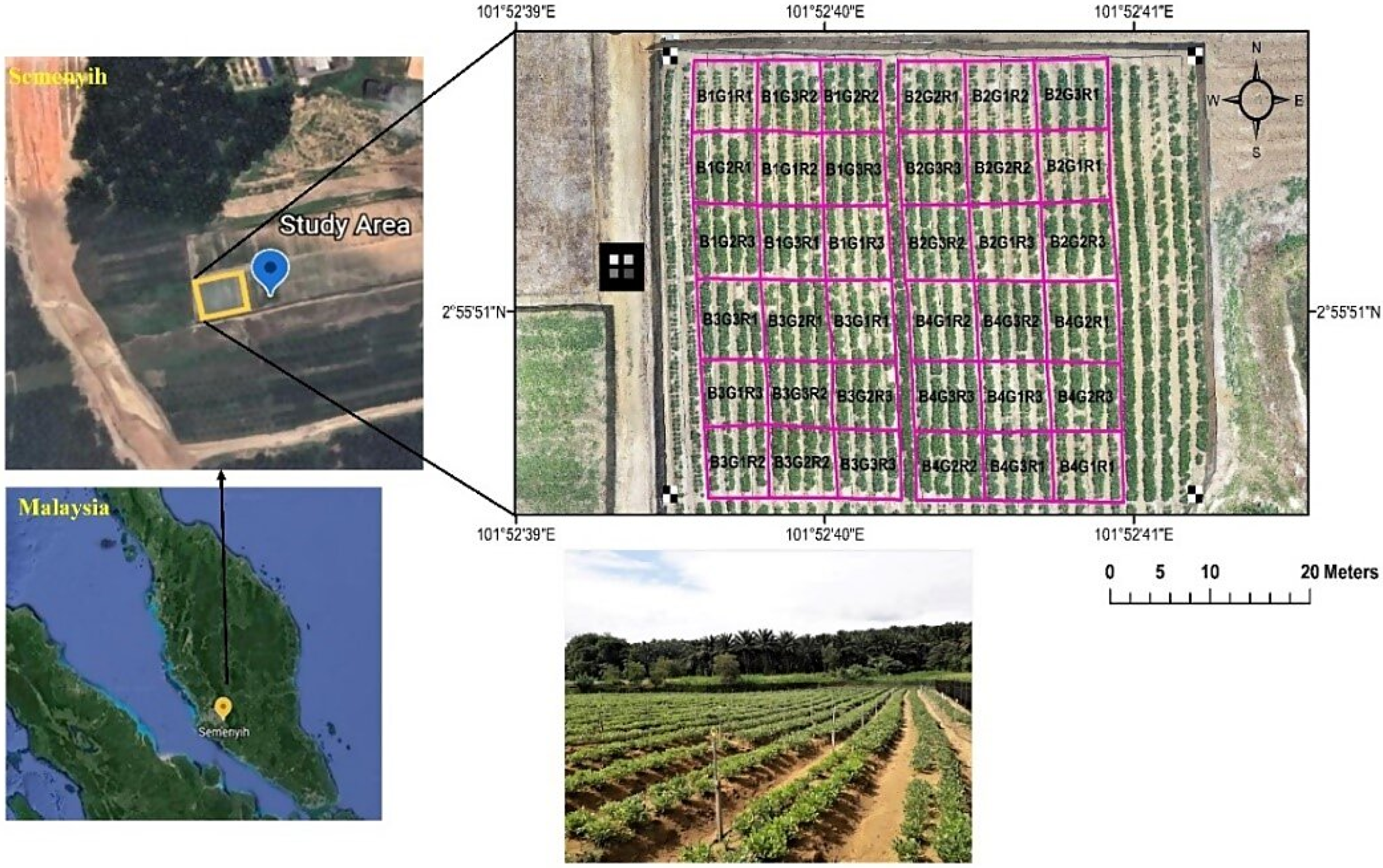
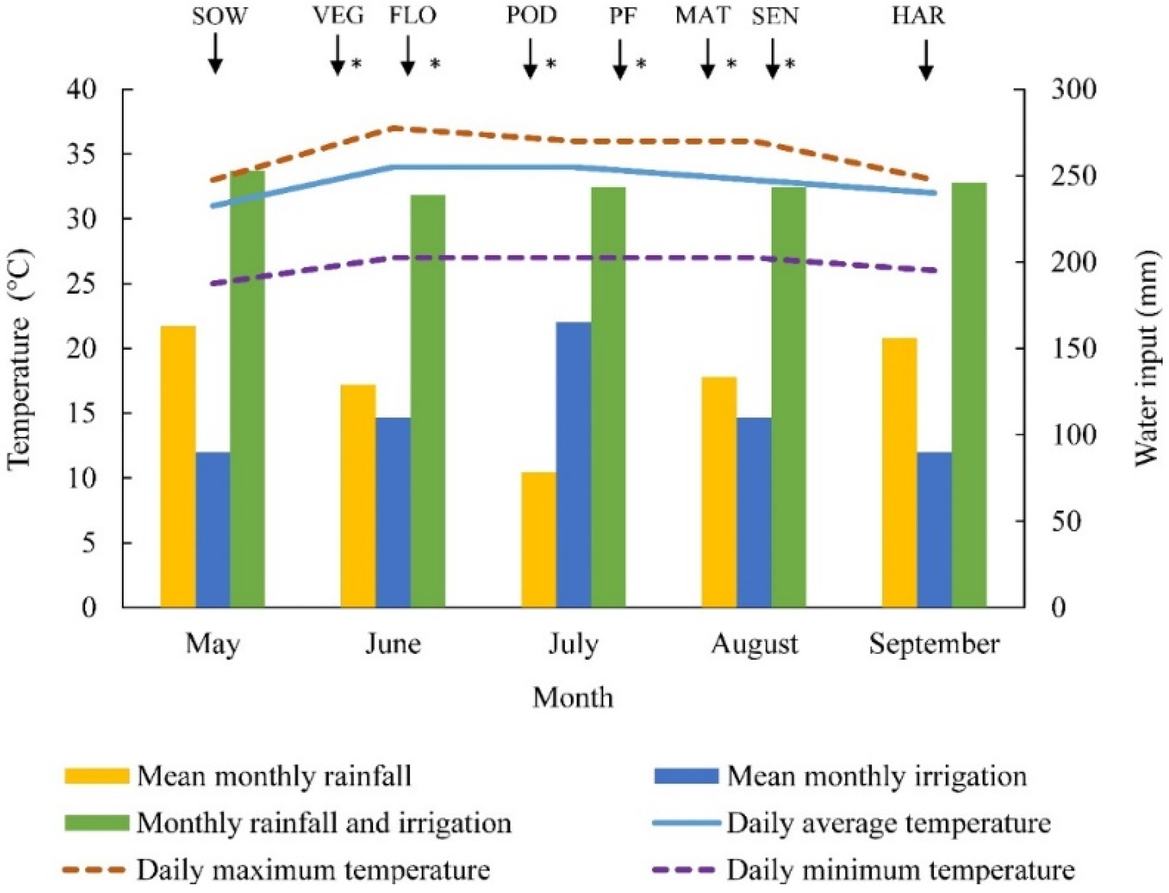
2.1. Study Site

The research was conducted at the Field Research Centre of Crops for the Future, located in Semenyih, Selangor, Malaysia. (2°55′56.96″ N, 101°52′33.59″ E), at 560 m above mean sea level from April to September 2018 (Figure 1).

The region exhibits a tropical climate, with an average annual temperature of 32.0 °C, an average annual precipitation of 1493 mm, and a typical photoperiod of 12 h day⁻¹. The environmental conditions recorded by the local weather station at the experimental site and the irrigation rates are shown in Figure 2.

2.2. Experimental Design

The field area covered approximately 0.2 ha with sandy clay loam soil with a pH value of 5.23. Three Bambara groundnut genotypes—NAV4 (genotype 1), IITA-686 (genotype 2), and CIVB (genotype 3)—were grown in a randomized complete block design across four blocks. Each block was subdivided into nine plots, with each genotype replicated three times within each block (Figure 1), resulting in 12 replications for each genotype (four blocks × three replicates per block). The gross plot size was 8 m by 7 m (56 m²), while the net plot area was 30 m² (6 m by 5 m). Row-to-row (inter-row) spacing between rows was set at 40 cm, and plant-to-plant (intra-row) spacing was 30 cm. The seeding rate for each genotype was 300,000 seeds ha⁻¹. Prior to sowing, a starter fertiliser was applied at a rate of 20:60:40 kg of nitrogen, phosphorus, and potassium, respectively. Sowing was conducted using a precision planter on 25 April 2018. Fungicides and insecticides were applied at regular intervals to manage pathogens, and weeding was performed manually using hand hoes. Throughout the trial, soil moisture content was monitored weekly using a soil moisture PR2 probe (Delta-T Devices Ltd., Cambridge, UK), and irrigation was initiated when soil water content decreased to 50% of the plant-available water capacity in the root zone.

2.3. Agronomic Measurements

Measurements of LAI, FVC, and CCC were conducted at various growth stages—days after sowing (DAS)—namely: vegetative (41 DAS), flowering (58 DAS), podding (84 DAS), pod-filling (97 DAS), maturity (105 DAS), and senescence (114 DAS) from May to September 2018. AGB assessments were made during the vegetative, flowering, podding, and senescence stages. Leaf area was determined using the LI-3100C Area Meter from LICOR (Lincoln, NE, USA), and LAI calculated by dividing the green leaf area by the sampled area. AGB was determined by harvesting all crops within a 1 m² area in the central rows at ground level and then drying the clippings for 120 h at 70 °C until a constant weight was achieved. Chlorophyll concentration (Chl) was measured using a SPAD-502 Plus device (Konica Minolta Sensing Inc., Tokyo, Japan) with SPAD units calibrated using the same methodology as described in [36]. CCC was estimated by multiplying the Chl per area values by the LAI. For FVC determination, digital images were captured and cropped to the area of interest (AOI) in ImageJ, with cropped images processed using the maximum likelihood supervised classification tool within ArcMap (ArcGIS^® by ESRI Inc., Redlands, AB, Canada). The zonal statistics tool was subsequently utilised to evaluate the number of “vegetated” pixels within each plot, and FVC was calculated by dividing the number of “vegetated” pixels by the total number of pixels in the AOI (refer to

Table 1. Summary statistics for Bambara groundnut canopy state variables. Min denotes the minimum value; Mean is the average value; Max indicates the maximum value; SD represents the standard deviation in the data; and CV (%) signifies the percent coefficient of variation. The sample size (N) for LAI, CCC, and FVC was 216 while N for AGB was 144.

Canopy State Variables	Min	Mean	Max	SD	CV (%)
LAI (m2 m−2)	1.39	2.79	4.19	1.40	50
AGB (ton ha−1)	0.59	1.46	2.33	0.87	60
CCC (mg m−2)	35.95	43.42	50.89	7.47	17
FVC (%)	14	32	50	18	57

for summary statistics).

2.4. UAV, Sensor and Remote Sensing Data Acquisition Missions

To enhance the reproducibility of our method, we utilised an affordable and readily available commercial UAV, the DJI Phantom 4 Pro (DJI Company, Shenzhen, China; website: https://www.dji.com/, accessed on 10 June 2020). This vertical take-off and landing (VTOL) quadcopter has a maximum payload capacity of 477 g and can sustain flight for 20–30 min, covering distances of up to 7 km. A Canon S100 camera (Canon, Tokyo, Japan), modified by MaxMax (LDP LLC, Carlstadt, NJ 07072, USA; website: www.maxmax.com, accessed on 10 June 2020), was mounted on the UAV using a two-axis aluminium–carbon–fibre gimbal set at nadir view (90° downward angle). This modification enabled the capture of colour infrared (CIR) digital imagery spanning the Green–Red–NIR spectrum (520–880 nm).

Six flight missions were conducted to obtain high-resolution images during crucial crop growth stages, including vegetative, flowering, podding, pod filling, maturity, and senescence. These flights were carried out under stable weather conditions from 10:00 to 14:00 local time to minimise variations in illumination. The flight paths and settings were predetermined using the DJI Ground Station Pro software 2.0 v.2.0.16, employing a moving-box flight path planning approach. To facilitate future image georectification, four ground control points (GCPs) were permanently positioned at each corner of the field. The accurate GPS coordinates of the GCPs were surveyed using a real-time kinematic (RTK)-enabled dual-frequency Leica 1200 Global Navigation Satellite System (GNSS) system with RTK precision (Leica Geosystems, Heerbrugg, Switzerland). Four 2 × 2 m calibration targets with nominal reflectance values of 10%, 20%, 50%, and 80% were utilised for radiometric calibration of the sensor. The spectral reflectance of these targets was measured using a handheld ASD spectroradiometer (FieldSpec, ASD, Boulder, CO, USA). Ultra high-resolution images were captured at a pre-scheduled flight altitude of 10 m, in nadir view, with a low flight speed of 0.5 m s⁻¹, and with an intended overlap of 75% in both in-track and cross-track directions to ensure sufficient overlapping coverage.

A Dell^® Inspiron 7000 laptop (Dell Technologies, Round Rock, TX, USA) was utilised with the Ground Controlling Station software 2.0 v.2.0.16 to manage the autonomous UAV flight via wireless network. The Canon S100 camera, set to TV mode for consistent shutter speed and aperture settings, was autonomously controlled to maintain optimal exposure levels. To automate camera functionality, the Canon CHDK free development software kit version 1.6.1, available at www.chdk.wiki.com, accessed 12 June 2020 was employed. The CHDK script enabled the UAV autopilot system to transmit electronic control signals, automating camera shutter triggering for precise data recording. During the data collection flight, auto-triggering occurred every 3 s (at a frequency of 0.33 Hz), facilitating the capture of approximately 400 images covering all plots within a 20 min flight duration, with a ground resolution of approximately 4 mm per pixel. The captured images were stored in 16-bit local digital memory cards as raw Geographic Tagged Image File Format files for subsequent image processing.

2.5. Image Processing

Following the flights, the raw images underwent pre-processing to eliminate electromagnetic interference in the visible bands from the NIR band, using Remote Sensing Explorer Software version 1.0 (MaxMax LDP LLC, Carlstadt, NJ, USA; www.maxmax.com, accessed 10 June 2020). Further pre-processing involved correcting lens distortion, chromatic aberration, and gamma correction using the Digital Photo Professional image processing software version 4.17.20 (Canon Inc., Tokyo, Japan; http://www.canon.co.uk/support/camera_software/, accessed 10 June 2020). The images were then imported into Agisoft Photoscan Pro Version 1.4.3 (Agisoft LLC, St. Petersburg, Russia) and mosaicked to create a single orthophotomosaic image for the entire study area for each flight date. The pixel size of the orthophotomosaics was approximately 4 mm per pixel to ensure high spatial resolution. Additionally, to minimise band-to-band misalignment, geometric correction was conducted on the orthophotomosaic using GCPs with surveyed GPS coordinates (Section 2.4). The georeferenced orthophotomosaic was subsequently brought into ArcMap Version 10.2.2 (ArcGIS^®, ESRI Inc., Redlands, AB, Canada; https://www.esri.com/en-us/arcgis/about-arcgis/overview, accessed 10 June 2020) for the co-registration of multi-temporal orthophotoimages. Radiometric correction was then applied to each orthophotomosaic for each flight date, band-by-band, to convert raw digital number (DN) values to reflectance values by employing a radiometric calibration equation developed between the known reflectance of the calibration targets and calibration target DN values in the empirical line correction method. Post-processing tasks included subsetting the area of interest (AOI) and digitising the quadrats using the ArcMap Editor tool. Geoprocessing steps also included resampling the images to a consistent pixel grid and correcting for any spatial misalignments between different flight dates. Finally, masks were applied to isolate the central portions of the canopy, excluding borders, and pure canopy pixels were utilised to compute average reflectance.

2.6. Vegetation Indices and Cumulative Vegetation Indices Calculation

After preprocessing, a set of five VIs was computed from the remotely sensed data (

Table 2. Vegetation indices (VIs) used in this study.

Index	Name	Formula	References
NDVI	Normalized difference vegetation index	(NIR − R)/(NIR + R)	[22]
GNDVI	Green normalized difference vegetation index	(NIR − G)/(NIR + G)	[25]
SR	Simple ratio	NIR/R	[24]
EVI2	Enhanced vegetation index 2	2.5 × (NIR − R)/(1 + NIR + 2.4 × R)	[26]
CIgreen	Green chlorophyll index	(NIR/G) − 1	[27]

Note: NIR, R, and G are the reflectance values of the near infrared, red, and green bands, respectively.

). These VIs were calculated for each orthophotomosaic using the ArcMap Raster Calculator tool, ArcMap Version 10.2.2 (ArcGIS^®, ESRI Inc., Redlands, AB, Canada; https://www.esri.com/en-us/arcgis/about-arcgis/overview, accessed 10 June 2020). Subsequently, the VIs were extracted on a quadrat-by-quadrat basis, and the mean, standard deviation and other statistics were generated using the ArcMap Zonal Statistics tool.

We evaluated three integration periods: from flowering to maturity, from flowering to senescence, and from vegetative to senescence. We calculated the ∑VIs over these integration periods using the same formula as in [8].

2.7. Model Selection and Modelling Strategy

We carefully selected the models to be used for estimating canopy state variables from VIs/ΣVIs. First, we assessed the dimensionality and multicollinearity of the dataset using principal component analysis (PCA) and variance inflation factor (VIF) analysis. Preliminary PCA results showed that a few principal components (PCs) captured most of the variance, suggesting the need for dimensionality reduction. This supported the decision to select models capable of handling high-dimensional data. High VIF values indicated the need for implementing models, which can deal effectively with multicollinearity. Furthermore, we examined residual plots and conducted tests to identify outliers and heteroscedasticity to inform our decision to select models, which are robust to outliers. Based on these assessments, we selected a diverse set of regression models that can effectively handle high dimensionality, multicollinearity, outliers, and overfitting.

We conducted Pearson’s correlation analysis between VIs/∑VIs and canopy state variables. The VIs from the optimal integration interval, based on the correlation analysis, were then utilised as input for both linear parametric and non-linear non-parametric regression models, including Huber Regressor (HR), Theil-Sen Regressor (TSR), AdaBoost Regressor (ABR), CatBoost Regressor (CBR), Multiple Linear Regression (MLR), Random Forest Regression (RFR), Partial Least Squares Regression (PLSR), and Ridge Regression (RR). HR is known for its robustness to outliers, which can indirectly help in datasets where outliers might exacerbate multicollinearity issues [37]. TSR, being a non-parametric method based on median calculations, is less sensitive to multicollinearity and offers robustness against certain types of data anomalies [38]. ABR, an ensemble method, can enhance model accuracy by combining multiple weak learners, providing a safeguard against overfitting, especially when the base estimator is appropriately chosen [39]. CBR, on the other hand, is designed to handle categorical features and high-dimensional data efficiently, with built-in mechanisms to prevent overfitting and address multicollinearity [40]. MLR uses regularisation (e.g., Ridge or Lasso) for overfitting, VIF for multicollinearity, and feature selection for high dimensionality [41]. RFR minimises overfitting with tree control, handles multicollinearity by subsampling, and addresses high dimensionality by feature selection [42]. PLSR reduces overfitting and multicollinearity through latent variables and manages high dimensionality by capturing essential information [43]. RR minimises overfitting using L2 regularisation, handles multicollinearity by redistributing variable influence, and reduces dimensionality effectively [44].

Prior to model implementation, the data were preprocessed for missing values, outliers capped, encoded, and normalised using Yeo–Johnson transformation. The dataset was split randomly into 80% training and 20% testing and scaled using StandardScaler from sklearn.preprocessing in a Python 3.9 environment (Python software version 3.9.0, Python Software Foundation, Wilmington, DE, USA). This was determined by experimenting with various splits: 50–50%, 60–40%, 70–30%, 80–20%, and 90–10%. The scikit-learn library was used for models such as HR, TSR, ABR, MLR, RFR, PLSR, and RR, utilising classes like HuberRegressor, TheilSenRegressor, AdaBoostRegressor, LinearRegression, RandomForestRegressor, PLSRegression, and RidgeRegression. For CBR, the CatBoostRegressor class from the catboost library was used. Hyperparameters were optimised using GridSearchCV from scikit-learn, which performs an exhaustive search over specified parameter values using cross-validation. Specifically, for each model, a range of hyperparameters was defined based on literature and preliminary results. The grid search involved training and validating models for each combination of hyperparameters in a five-fold cross-validation setup, ensuring robustness and preventing overfitting. The best hyperparameters were selected based on the highest average cross-validated score, ensuring optimal model performance (

Table 3. Hyperparameters evaluated for optimising the ML models.

Model	Hyperparameter	Description	Values Evaluated	Selected Hyperparameter
HR	epsilon	Tolerance to outliers	0.01, 0.1, 0.5, 1.0, 2.0	0.1
	max_iter	Maximum iterations for optimisation	100, 200, 500, 1000	500
	alpha	Regularisation strength	0.0001, 0.001, 0.01, 0.1, 1.0	0.01
	warm_start	Reuse previous solution	True, False	False
TSR	n_subsamples	Number of subsets for robust estimation	100, 200, 500, 1000	500
	max_iter	Maximum iterations for optimisation	100, 200, 500, 1000	1000
ABR	n_estimators	Number of weak learners (trees)	50, 100, 200, 500	200
	learning_rate	Scaling factor for weak learners	0.01, 0.1, 0.5, 1.0	0.1
CBR	iterations	Number of boosting iterations (trees)	100, 200, 500, 1000	500
	learning_rate	Step size for adaptation during training	0.01, 0.05, 0.1, 0.2	0.1
	depth	Maximum depth of trees in the ensemble	4, 6, 8, 10	6
	l2_leaf_reg	L2 regularisation for leaf values	1.0, 5.0, 10.0	5.0
MLR	n/a	n/a	n/a	n/a
RFR	n_estimators	Number of trees in the forest	10, 50, 100, 200	100
	max_depth	Maximum depth of each tree	None, 10, 20, 30	20
	min_samples_split	Minimum number of samples to split a node	2, 5, 10	2
	min_samples_leaf	Minimum number of samples in a leaf node	1, 2, 4	1
PLSR	n_components	Number of components to keep	1, 2, 3, 4	3
	scale	Whether to scale the data	True, False	True
RR	alpha	Regularisation strength	0.1, 1.0, 10.0	1.0
	solver	Algorithm to use in the optimisation	‘auto’, ‘svd’, ‘cholesky’, ‘lsqr’, ‘saga’	auto

).

The models were trained on the training data, and their performances were evaluated on the testing data using metrics such as the coefficient of determination (R²), Root Mean Squared Error (RMSE), Root Mean Squared Error Percentage (RMSE%), Mean Absolute Error (MAE), Mean Squared Error (MSE), and Mean Absolute Percentage Error (MAPE). The predicted versus observed values and predictor importance plots were generated using the best model on the testing dataset. To identify the predictors that most significantly contribute to prediction models, we conducted a variable importance analysis. The importance of each predictor was determined by calculating its R² and ranking the indices from highest to lowest R² values. A workflow showing the main steps in modelling Bambara groundnut canopy state variables is shown in Figure 3.

3. Results and Discussion

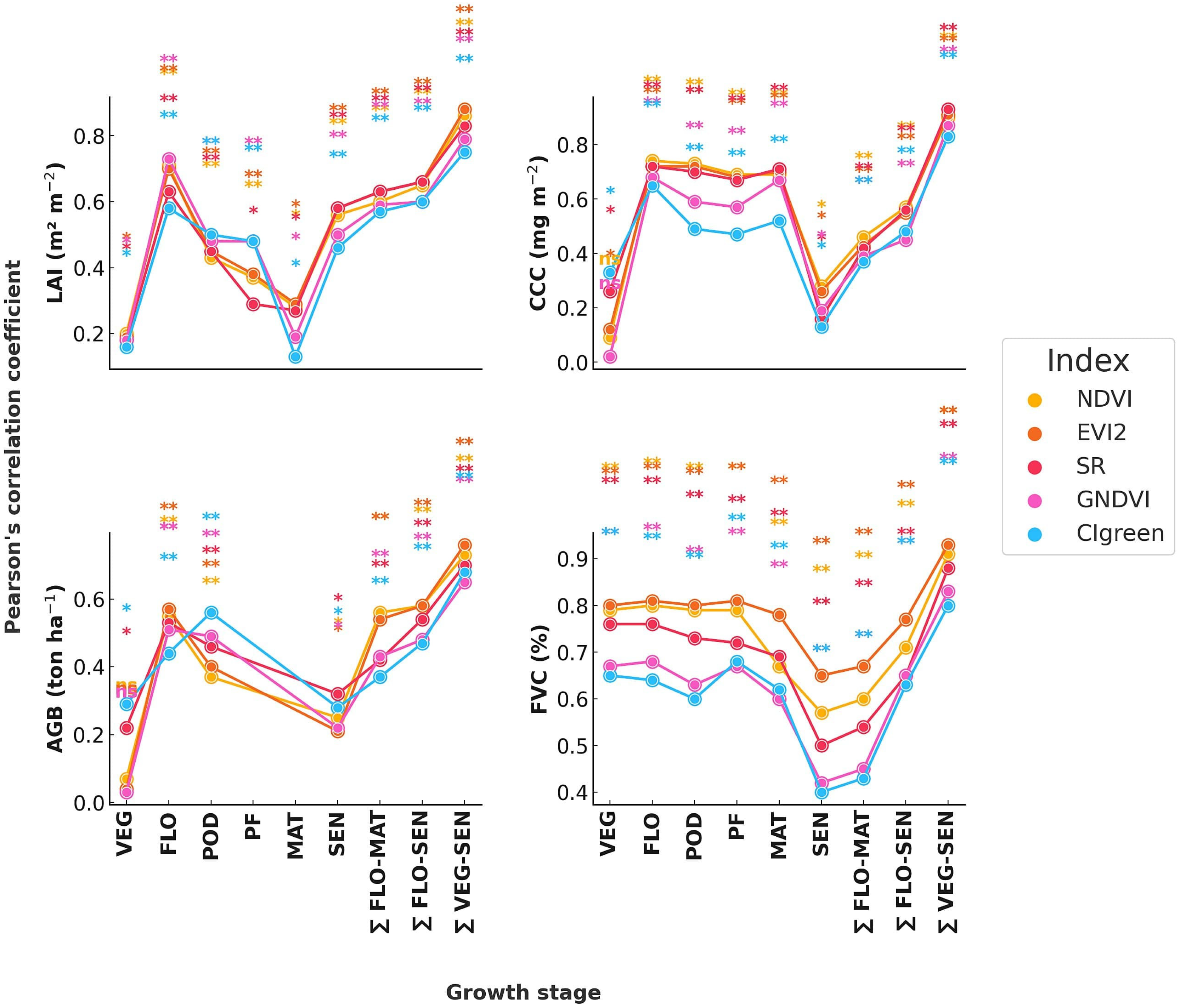
3.1. Correlation of Canopy State Variables with Vegetation Indices and Cumulative Vegetation Indices

Figure 4 shows strong correlations between LAI, CCC, AGB, and VIs at each growth stage, except during the vegetative and senescence stages. FVC exhibited strong correlations with VIs at all stages except senescence stage.

The low correlation observed during the vegetative stage can be attributed to low LAI and high background reflectance. LAI is crucial in linking VIs to agronomic measurements, particularly in the red and NIR spectral bands, which are sensitive to changes in aboveground biomass [45]. The overall trend shows correlation increasing from the vegetative to the flowering stage, then declining from flowering to senescence, with peak values in LAI, CCC, FVC, and AGB observed at flowering. This trend is consistent with the findings of Tan et al. [46] who reported that VIs effectively estimate maize LAI, with the best results observed from the bell stage to the silking stage, when LAI experiences significant changes. Similarly, another study also highlighted the effectiveness of hyperspectral VIs in monitoring LAI across different growth stages of cotton [47]. Similar variation in correlation between VIs and maize leaf chlorophyll content (LCC) throughout the growing season was reported by Yang et al. [48]. Moreover, they reported that correlation between VIs and LCC varied significantly vertically in the upper and lower leaf layers during the early vegetative and maturity stages.

Our results show that FVC exhibited strong correlations with all VIs across most growth stages, confirming the effectiveness of VIs as indicators of vegetation cover. This finding aligns with a study on soybean growth dynamics, which also highlighted the potential of VIs in analysing vegetation cover and vigour [49]. However, several complexities and confounding factors explain the weaker correlations between AGB and VIs compared to LAI, FVC, and CCC. Factors such as canopy structure, water content, and aboveground biomass distribution heterogeneity contribute to this weaker correlation. A recent study emphasised the importance in combining various VIs and canopy texture parameters for more accurate estimation of rice AGB. When both VIs and canopy structure parameters were combined, there was an improvement in the estimation accuracy [50].

The correlation declines as the canopy undergoes leaf withering and shedding from flowering to senescence. This results in reduced LAI, FVC, AGB, and CCC, alongside an increase in carotenoid content, thus decreasing correlation. Similar patterns were observed in wheat [51] and maize [52]. Our study reveals that ∑VIs, from vegetative to senescence stages, exhibit stronger correlations with canopy state variables compared to single-stage VIs. Integrating VIs over time better captures canopy photosynthetic capacity, indicative of potential dry matter production. Models predicting maize yield based on ∑VIs (VI-SUMs) and VIs by area under the curve (VI-AUCs) demonstrated better stability and accuracy (R² = 60–65%) [53]. This is comparable to Su et al. [54], who estimated rice yield using ∑VIs and leaf panicle abundance (R² = 0.73, RRMSE = 0.22 and R² = 0.75, RRMSE = 0.15, respectively).

Additionally, our findings indicate that VIs composed of red and NIR bands exhibit stronger correlations with canopy state variables than VIs composed of NIR and green bands. This aligns with the well-known phenomenon of vegetation absorbing red bands more effectively and reflects NIR bands strongly. This observation is also supported by studies on other crops, such as wheat and soybean, which reported higher accuracy in biomass estimation using red and NIR bands [55,56,57].

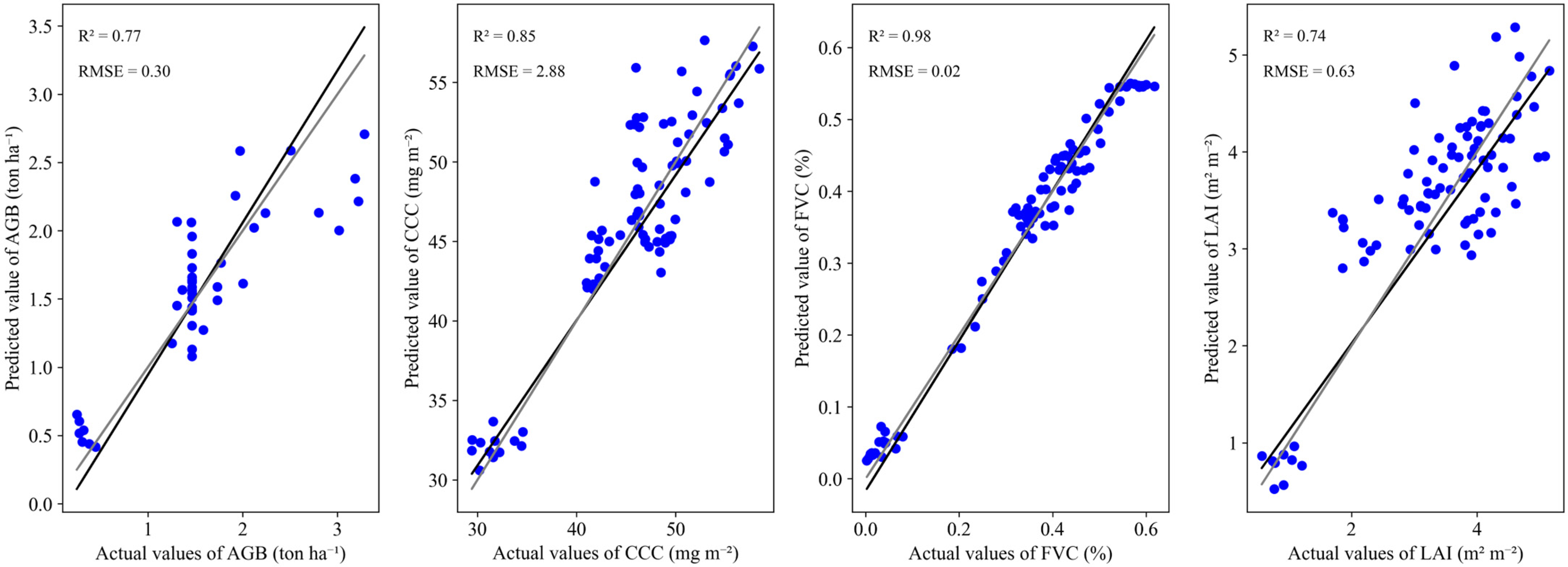
3.2. Modeling the Relationship between Canopy State Variables and Cumulative Vegetation Indices Using Machine-Learning Algorithms

Table 4. Evaluation metrics for estimating canopy state variables using various models: CBR (CatBoostRegressor), TSR (TheilSen Regressor), ABR (AdaBoost Regressor), HR (Huber Regressor), MLR (Multiple Linear Regressor), RFR (Random Forest Regressor), PLSR (Partial Least Squares Regressor), and RR (Ridge Regressor). The best-performing models in testing are indicated using bold font.

	Model	CBR		TSR		MLR		RR		PLSR		RFR		ABR		HR
	Data	Train	Test	Train	Test	Train	Test	Train	Test	Train	Test	Train	Test	Train	Test	Train	Test
AGB	R2	0.99	0.55	0.47	0.66	0.65	0.77	0.27	0.49	0.04	0.21	0.91	0.57	0.90	0.47	0.50	0.66
	RMSE	0.04	0.39	0.39	0.31	0.37	0.30	0.46	0.38	0.51	0.46	0.19	0.40	0.21	0.42	0.39	0.33
	RMSE%	3	27	26	21	25	20	31	26	34	31	13	27	14	28	26	22
	MAE	0.03	0.25	0.23	0.22	0.24	0.23	0.29	0.27	0.33	0.31	0.10	0.27	0.16	0.28	0.22	0.22
	MSE	0.00	0.16	0.15	0.10	0.14	0.09	0.21	0.15	0.26	0.21	0.04	0.16	0.04	0.18	0.15	0.11
	MAPE	2	17	16	15	16	18	22	21	23	22	5	16	11	19	15	17
CCC	R2	0.99	0.83	0.84	0.83	0.84	0.83	0.83	0.81	0.81	0.78	0.98	0.85	0.93	0.82	0.84	0.82
	RMSE	0.25	2.91	3.06	3.10	2.87	2.97	2.94	3.11	3.09	3.30	1.01	2.88	1.98	2.91	2.88	3.06
	RMSE%	1	6	7	7	6	6	6	7	7	7	2	6	4	6	6	7
	MAE	0.21	2.29	2.42	2.43	2.27	2.35	2.33	2.52	2.45	2.69	0.74	2.29	1.70	2.28	2.26	2.40
	MSE	0.07	8.46	9.34	9.58	8.23	8.84	8.65	9.66	9.53	10.89	1.03	8.31	3.93	8.48	8.31	9.34
	MAPE	1	5	5	5	5	5	5	6	5	6	2	5	4	5	5	5
FVC	R2	0.99	0.97	0.98	0.98	0.98	0.98	0.98	0.97	0.98	0.97	0.99	0.98	0.99	0.97	0.98	0.98
	RMSE	0.00	0.03	0.02	0.03	0.02	0.03	0.02	0.03	0.03	0.03	0.01	0.02	0.02	0.03	0.02	0.03
	RMSE%	1	7	6	8	6	7	6	8	7	8	3	6	5	7	6	7
	MAE	0.00	0.02	0.02	0.02	0.02	0.02	0.02	0.02	0.02	0.02	0.01	0.02	0.02	0.02	0.02	0.02
	MSE	0.00	0.00	0.00	0.00	0.00	0.00	0.00	0.00	0.00	0.00	0.00	0.00	0.00	0.00	0.00	0.00
	MAPE	1	11	31	24	16	25	18	17	42	13	3	10	9	11	24	24
LAI	R2	0.99	0.70	0.79	0.73	0.80	0.74	0.79	0.74	0.72	0.71	0.97	0.55	0.91	0.69	0.79	0.74
	RMSE	0.08	0.64	0.58	0.65	0.56	0.63	0.57	0.62	0.64	0.66	0.21	0.74	0.39	0.65	0.56	0.63
	RMSE%	2	19	18	20	17	19	17	19	19	20	6	22	12	20	17	19
	MAE	0.06	0.52	0.45	0.50	0.43	0.48	0.44	0.48	0.51	0.53	0.16	0.60	0.33	0.52	0.43	0.49
	MSE	0.01	0.42	0.34	0.42	0.31	0.40	0.32	0.39	0.41	0.43	0.04	0.54	0.15	0.42	0.32	0.40
	MAPE	3	18	16	17	15	16	16	16	18	21	6	21	11	18	15	17

and Figure 5 show performance results of predictive models in both training and testing.

For AGB, the gradient boosting CBR displayed an impressive training accuracy, but its performance in testing was moderate, suggesting potential overfitting. While our study employed CBR, other studies have also highlighted the efficacy of other gradient boosting algorithms such as the grasshopper optimisation algorithm-driven XGBoost (GOA-XGB) model which accurately predicted wheat AGB using multispectral bands and VIs. GOA-XGB outperformed other models, with RMSE of 0.226 kg m⁻² and R² of 0.855 [58]. MLR and TSR, on the other hand, showed a more consistent performance between training and testing, making them better performing models in terms of errors. Linear regression models, in general, have been foundational in many agronomy studies due to their interpretability. RFR and ABR both exhibited high training accuracies, but their testing performances were lower. Similarly, Wai et al. [59] employed Sentinel-2 Multispectral Instrument (MSI) derivatives and Shuttle Radar Topographic Mission (SRTM) Digital Elevation Model (DEM) together with field data and ML techniques to estimate AGB of evergreen and deciduous forest in Myanmar. They found that RFR and the gradient boosting algorithm provided moderate results (validation R² = 0.47, RMSE = 24.91 t/ha and R² = 0.52, RMSE = 34.72 t/ha). Their findings suggested that these models hold significant potential in estimating AGB. In a comparative study on AGB in plantation forests, Stochastic Gradient Boosting (SGB) outperformed RFR, especially when applied to a combined species dataset. This highlights the importance of appropriate model selection based on the specific dataset and ecological context [60]. In our study, simpler models like PLSR, RR, and HR had varied performances, indicating they might not be the best fit for this particular dataset. RR performance can be influenced by its regularisation parameter, potentially leading to overfitting or underfitting. PLSR performance can be influenced by the number of latent variables used and the nature of relationships between predictors and the response variable. A study by Ohsowski et al. [61] highlighted these issues with RR and PLSR in estimating forest AGB. HR for instance is influenced by its epsilon parameter which determines its sensitivity to outliers in the dataset [37]. These results indicate the importance of careful model tuning prior to modelling.

For CCC, in training the ensemble models CBR and RFR, exhibited similar strong performance, however, in testing RFR achieved a higher R² than CBR. This was followed by ABR with a slightly lower performance in testing. Zhang et al. [62] employed several ensemble learning algorithms including RFR, gradient boosting decision tree (GBDT), extreme gradient boosting (XGBoost), light gradient boosting machine (LightGBM), and CBR to estimate chlorophyll-a content in water bodies using hyperspectral data. They reported that XGBoost outperformed the other models in estimating chlorophyll-a content (R² = 0.8351, RMSE = 6.6477 μg/L). The enhanced performances of ensemble models are due to their capacity to capture complex non-linear relationships, they are robust to noise, can handle multicollinearity, and maintain balance between bias and variance. Moreover, ensemble models combine predictions from multiple base models, hence providing better generalisation of unseen data [62]. In our study, MLR, RR, TSR PLSR, and HR, had similar performance in predicting CCC. It is worth noting that these models displayed more stable performance when comparing training and testing. Ensemble models are often considered as “black-box” models as their decision-making processes are less interpretable than simpler models which provide a coefficient-based equation [63]. Thus, it might be simpler to implement linear models to estimate groundnut canopy state variables.

In prediction of FVC, all models had similar performance (similar R² and error evaluation metrics) with RFR performing slightly better in testing. This is consistent with findings from a study that employed a combination of VIs derived from Sentinel-2 and UAV images together with ML algorithms for wheat and sugarcane FVC estimation in India. They reported that RFR and k-nearest neighbor (KNN) outperform support vector regression (SVR) and linear regressor. The RFR model achieved highest R² values ranging from 0.862 to 0.873 when different VIs are used as input features. Another study employed UAV imagery and three models including RFR, artificial neural network (ANN), and MLR to estimate maize FVC under varying irrigation levels [64]. Results indicate that RFR was the most accurate, especially for different growth stages and water stress conditions, while MLR performed poorly for high FVC levels. However, the authors pointed to the need to test the developed models on the same crop and other crops in different locations across several growing seasons.

For LAI, the ensemble models CBR, RFR, and ABR had impressive training performance while testing performance was lower. This is indicative of potential overfitting. This is consistent with the findings of Martinez et al. [65] where they explored the use of satellite-derived VIs together with linear, non-linear, decision trees and RFR algorithms to model mangrove forests. Although their results indicated the ensemble RFR model to be the best performing with lowest RMSE, they highlighted the potential of overfitting. As observed previously, TSR, MLR, PLSR, HR, and RR had more stable performance comparing training and testing evaluation metrics. Although MLR performed best in testing there was not much difference. This suggest that these models generalise better on unseen data in testing. This corroborates with a study on soybean phenotyping where multimodal UAV hyperspectral, multispectral, and LiDAR, data collected at three growth stages were used as input to six algorithms including MLR, RFR, XGBoost, SVM, and back propagation (BP) for the estimation of LAI [66]. Although their results indicate that XGBoost and RFR had better performances in validation (R² of 0.762, RMSE of 0.236 and R² of 0.737, RMSE of 0.277, respectively) it was not much different from MLR (R² of 0.649 and RMSE of 0.253).

To conclude, models like CBR, RFR, and ABR showed highest performance in training for estimation of groundnut canopy state variables, indicating their enhanced capacity to capture complex relationships and patterns in the data. However, as highlighted before, the performance was significantly lower in testing which might indicate the need for careful hyperparameter tuning and feature engineering to minimise potential overfitting. Moreover, high model complexity, insufficient training data, noisy data, and lack of cross-validation might also contribute to overfitting. Models like MLR, TSR, PLSR, HR, and RR showed more consistent performance between training and testing, suggesting their reliability in estimating groundnut canopy state variables. These models are reliable choices which might be worthy of consideration in future modelling of agronomic variables.

3.3. Predictor Importance for Estimating Bambara Groundnut Canopy State Variables

As shown in Figure 6, for AGB, the ranking of feature importance is GNDVI (most important), CI_green, NDVI, SR, and EVI2 (least important).

In CCC estimation, SR leads, followed by NDVI and GNDVI, with EVI2 and CI_green being least important. For FVC, CI_green is most crucial, then NDVI and GNDVI, with SR and EVI2 as least important. Lastly, in LAI estimation, GNDVI is most important, followed by EVI2 and NDVI (similar importance), then CI_green, and SR (least important).

In accordance with our findings, Gitelson and Merzlyak [67], highlighted that GNDVI differs from NDVI by substituting the red band with the green band, resulting in increased sensitivity to changes in chlorophyll concentration. This substitution of bands has led to enhancements in estimation. Our findings are consistent with the work of Sankaran et al. [68], who demonstrated strong correlations between GNDVI and seed yield, as well as biomass. Additionally, Macedo et al. [69] found a robust relationship between GNDVI and corn crop productivity, further emphasizing the importance of GNDVI in AGB estimation. In addition to GNDVI, other VIs have also been extensively studied for AGB estimation. For instance, Liu et al. [70] demonstrated the estimation of potato AGB based on UAV red–green–blue images using different texture features and crop height. Tao et al. [71] found significant correlations between VIs, red-edge parameters, and AGB, highlighting the potential for improved AGB estimation using a combination of these parameters. Furthermore, the integration of RS data, such as LiDAR and optical sensors, has been shown to enhance AGB estimation [72].

Similar to our results, SR was identified as having the best predictive performance for estimating canopy level chlorophyll content [73]. Additionally, the red-edge region of the electromagnetic spectrum showed strong potential for estimating CCC [74]. Furthermore, the red-edge chlorophyll index (CI_red-edge) was found to be a good and linear estimator of CCC in different cropping systems [75]. The relevance of these indices in estimating CCC was further supported by studies that utilised in situ measurements of spectral reflectance, biophysical characteristics, and ecosystem CO₂ fluxes to estimate CCC [76]. It is important to note that the effectiveness of these indices in estimating CCC was studied not only at the canopy level but also at the leaf scale. For instance, the relationship between leaf chlorophyll content and canopy reflectance was explored, indicating the potential for accurately extrapolating leaf-scale indices to the canopy level [77].

In the estimation of FVC, CI_green emerges as the most important index, outperforming others in robustness and suitability, similar to the results of Thanyapraneedkul et al. [78]. NDVI and GNDVI also played significant roles, showing strong linear relationships with FVC across various environmental conditions [76,77]. Conversely, indices like SR and EVI2 were found to be less effective in predicting Bambara groundnut FVC. Similar studies by Viña et al. [79] and Luscier et al. [80] indicated that these indices had lower predictive performance and are recommended less frequently for monitoring vegetation biophysical characteristics. This suggests that the selection of appropriate VIs is critical for accurate and reliable FVC estimation.

Our results revealed that GNDVI was the best index for estimating Bambara groundnut LAI. The importance of GNDVI for LAI estimation is supported by Dai et al. [81], who found that GNDVI, along with other indices such as EVI and Soil Adjusted Vegetation Index (SAVI), exhibited higher correlations with LAI compared to NDVI. EVI2 and NDVI have also been highlighted as important indices for LAI estimation. Fang et al. [82] discussed the widespread use of NDVI for LAI estimation, indicating its significance in this context. Kang et al. [83] emphasised the comparable performance of EVI2 and EVI in LAI estimation at global scales, further underlining the importance of these indices. On the other hand, our results indicate CI_green and SR were identified as the least important indices for Bambara groundnut LAI estimation. This is supported by the study of Stenberg et al. [84] who found that CI_green and SR exhibited poor sensitivity to changes in LAI due to saturation. In conclusion, the importance of VIs for LAI estimation varies, with GNDVI being the most important, followed by EVI2 and NDVI, with CI_green and SR being the least important.

4. Limitations and Future Perspectives

A limitation of our study is the restricted temporal scope, focusing on data from 2018–2019. Key crop growth information is influenced by multiple factors such as environment and temperature, necessitating a longer period of data collection to capture inter-annual variability. Moreover, expanding the study to cover more regions and a wider range of genotypes is crucial for comparative analysis and generalisation of the findings. Such comprehensive data would allow for a more robust understanding of crop growth dynamics and the development of models that are resilient across different environmental conditions and genetic variations.

Another significant challenge in our study is the underlying issue of overfitting. To mitigate overfitting in ML modelling, several techniques have been proposed. One of the main methods is k-fold cross-validation, which assesses model performance on different subsets of the data to ensure generalisation [85]. Feature selection is another technique whereby irrelevant features are eliminated to reduce model complexity [86]. Regularisation techniques, such as L1 (Lasso) or L2 (Ridge), which penalise large coefficients aiming to simplify models are also effective. Novel methods like L1/4 regularisation can address both overfitting and underfitting [87]. Another technique is monitoring model performance on a validation set and employing early stopping when performance deteriorates. Data augmentation techniques, for example synthetic data augmentation for tabular data (SMOTE), generative adversarial networks (GAN), and combined use of SMOTE and GAN, can effectively increase training dataset size thereby increasing model variations and handling concerns of overfitting and loss of generalisation [88]. Moreover, ensemble models, such as RFR and gradient boosting regressor, have been shown to offer high resilience against overfitting. However, opting for simpler models or reducing the complexity of the models are beneficial, as observed in our results. Finally, fine-tuning hyperparameters can effectively minimise both underfitting and overfitting.

Future studies should explore the use of Explainable artificial intelligence to understand the decision-making mechanisms models and interactions among various indices and algorithms. The integration of data from various in situ and other sources, such as meteorological data, field ancillary data, and real-time data, has the potential to enhance understanding and improve prediction accuracy. In addition, the utilisation of advanced deep learning methodologies, such as convolutional neural networks, has promise in the extraction of features from RS data, thereby improving prediction accuracy. Moreover, multispectral and hyperspectral data, in conjunction with the abovementioned data, have the potential to provide a comprehensive understanding of crop growth and development. Future studies should explore the integration of radiative transfer models with deep learning for gauging the estimation of crop state variables. Such hybrid methods combine both the strengths of process-based and data-driven models for scalable, accurate, and robust prediction models.

5. Conclusions

The study investigated correlations between LAI, AGB, FVC, and CCC with VIs/∑VIs obtained at single stages and over combinations of stages. The highest single-stage correlation was observed at flowering, while ∑VIs spanning from vegetative to senescence showed the strongest correlations with all canopy state variables. Although ensemble models performed well in training across all canopy state variables, they exhibited signs of potential overfitting during testing. In contrast, simpler models consistently provided reliable results in both training and testing. Our results show that MLR is particularly effective for AGB and LAI estimation, while RFR shows superior performance for CCC and FVC estimation. Our findings highlight GNDVI as the most crucial index for estimating Bambara groundnut AGB and LAI, while SR proves optimal for CCC and CI_green for FVC, underlining the importance of careful VI selection in canopy state variable estimation. In conclusion, our study demonstrates that VIs derived from images captured by digital cameras mounted on low-cost UAVs, together with machine learning algorithms, can accurately estimate Bambara groundnut canopy state variables.

References

1. Li, X.; Yadav, R.; Siddique, K.H.M. Neglected and Underutilized Crop Species: The Key to Improving Dietary Diversity and Fighting Hunger and Malnutrition in Asia and the Pacific. Front. Nutr. 2020, 7, 593711. [Google Scholar] [CrossRef] [PubMed]
2. Padulosi, S.; Heywood, V.; Hunter, D.; Jarvis, A. Underutilized Species and Climate Change: Current Status and Outlook. In Crop Adaptation to Climate Change; Wiley-Blackwell: Oxford, UK, 2011; pp. 507–521. [Google Scholar]
3. Tan, X.L.; Azam-Ali, S.; Von Goh, E.; Mustafa, M.; Chai, H.H.; Ho, W.K.; Mayes, S.; Mabhaudhi, T.; Azam-Ali, S.; Massawe, F. Bambara Groundnut: An Underutilized Leguminous Crop for Global Food Security and Nutrition. Front. Nutr. 2020, 7, 601496. [Google Scholar] [CrossRef] [PubMed]
4. Soumare, A.; Diedhiou, A.G.; Kane, A. Bambara groundnut: A neglected and underutilized climate-resilient crop with great potential to alleviate food insecurity in sub-Saharan Africa. J. Crop Improv. 2022, 36, 747–767. [Google Scholar] [CrossRef]
5. Chibarabada, T.P.; Modi, A.T.; Mabhaudhi, T. Options for improving water productivity: A case study of bambara groundnut and groundnut. Phys. Chem. Earth Parts A/B/C 2020, 115, 102806. [Google Scholar] [CrossRef]
6. Mayes, S.; Ho, W.K.; Chai, H.H.; Gao, X.; Kundy, A.C.; Mateva, K.I.; Zahrulakmal, M.; Hahiree, M.K.I.M.; Kendabie, P.; Licea, L.C.S.; et al. Bambara groundnut: An exemplar underutilised legume for resilience under climate change. Planta 2019, 250, 803–820. [Google Scholar] [CrossRef]
7. Linneman, A. Phenological Development in Bambara Groundnut (Vigna subterranea) at Constant Exposure to Photoperiods of 10 to 16 h. Ann. Bot. 1993, 71, 445–452. [Google Scholar] [CrossRef]
8. Jewan, S.Y.Y.; Pagay, V.; Billa, L.; Tyerman, S.D.; Gautam, D.; Sparkes, D.; Chai, H.H.; Singh, A. The feasibility of using a low-cost near-infrared, sensitive, consumer-grade digital camera mounted on a commercial UAV to assess Bambara groundnut yield. Int. J. Remote. Sens. 2021, 43, 393–423. [Google Scholar] [CrossRef]
9. Qi, H.; Zhu, B.; Wu, Z.; Liang, Y.; Li, J.; Wang, L.; Chen, T.; Lan, Y.; Zhang, L. Estimation of Peanut Leaf Area Index from Unmanned Aerial Vehicle Multispectral Images. Sensors 2020, 20, 6732. [Google Scholar] [CrossRef] [PubMed]
10. Zhang, J.; Sun, H.; Gao, D.; Qiao, L.; Liu, N.; Li, M.; Zhang, Y. Detection of Canopy Chlorophyll Content of Corn Based on Continuous Wavelet Transform Analysis. Remote Sens. 2020, 12, 2741. [Google Scholar] [CrossRef]
11. Fu, Y.; Yang, G.; Song, X.; Li, Z.; Xu, X.; Feng, H.; Zhao, C. Improved Estimation of Winter Wheat Aboveground Biomass Using Multiscale Textures Extracted from UAV-Based Digital Images and Hyperspectral Feature Analysis. Remote Sens. 2021, 13, 581. [Google Scholar] [CrossRef]
12. Zhang, S.; Chen, H.; Fu, Y.; Niu, H.; Yang, Y.; Zhang, B. Fractional Vegetation Cover Estimation of Different Vegetation Types in the Qaidam Basin. Sustainability 2019, 11, 864. [Google Scholar] [CrossRef]
13. Feng, L.; Chen, S.; Zhang, C.; Zhang, Y.; He, Y. A comprehensive review on recent applications of unmanned aerial vehicle remote sensing with various sensors for high-throughput plant phenotyping. Comput. Electron. Agric. 2021, 182, 106033. [Google Scholar] [CrossRef]
14. Yang, G.; Liu, J.; Zhao, C.; Li, Z.; Huang, Y.; Yu, H.; Xu, B.; Yang, X.; Zhu, D.; Zhang, X.; et al. Unmanned aerial vehicle remote sensing for field-based crop phenotyping: Current status and perspectives. Front. Plant Sci. 2017, 8, 272832. [Google Scholar] [CrossRef] [PubMed]
15. Tattaris, M.; Reynolds, M.P.; Chapman, S.C. A direct comparison of remote sensing approaches for high-throughput phenotyping in plant breeding. Front. Plant Sci. 2016, 7, 206105. [Google Scholar] [CrossRef] [PubMed]
16. Ma, Z.; Rayhana, R.; Feng, K.; Liu, Z.; Xiao, G.; Ruan, Y.; Sangha, J.S. A Review on Sensing Technologies for High-Throughput Plant Phenotyping. IEEE Open J. Instrum. Meas. 2022, 1, 9500121. [Google Scholar] [CrossRef]
17. Sharma, L.K.; Gupta, R.; Pandey, P.C. Future Aspects and Potential of the Remote Sensing Technology to Meet the Natural Resource Needs. In Advances in Remote Sensing for Natural Resource Monitoring; Springer: Cham, Switzerland, 2021; pp. 445–464. [Google Scholar]
18. Weiss, M.; Jacob, F.; Duveiller, G. Remote sensing for agricultural applications: A meta-review. Remote Sens. Environ. 2020, 236, 111402. [Google Scholar] [CrossRef]
19. Naveed Tahir, M.; Lan, Y.; Zhang, Y.; Wang, Y.; Nawaz, F.; Arslan Ahmed Shah, M.; Gulzar, A.; Shahid Qureshi, W.; Manshoor Naqvi, S.; Zaigham Abbas Naqvi, S. Real time estimation of leaf area index and groundnut yield using multispectral UAV. Int. J. Precis. Agric. Aviat. 2018, 1, 1–6. [Google Scholar] [CrossRef]
20. Li, B.; Xu, X.; Zhang, L.; Han, J.; Bian, C.; Li, G.; Liu, J.; Jin, L. Above-ground biomass estimation and yield prediction in potato by using UAV-based RGB and hyperspectral imaging. ISPRS J. Photogramm. Remote Sens. 2020, 162, 161–172. [Google Scholar] [CrossRef]
21. Chen, J.; Yi, S.; Qin, Y.; Wang, X. Improving estimates of fractional vegetation cover based on UAV in alpine grassland on the Qinghai–Tibetan Plateau. Int. J. Remote Sens. 2016, 37, 1922–1936. [Google Scholar] [CrossRef]
22. Rouse, J.W.J.; Haas, R.H.; Deering, D.W.; Schell, J.A.; Harlan, J.C. Monitoring the Vernal Advancement and Retrogradation (Green Wave Effect) of Natural Vegetation; NASA/GSFC Type III Final Report; NASA: Greenbelt, MD, USA, 1974. [Google Scholar]
23. Shamsuzzoha, M.; Noguchi, R.; Ahamed, T. Rice Yield Loss Area Assessment from Satellite-derived NDVI after Extreme Climatic Events Using a Fuzzy Approach. Agric. Inf. Res. 2022, 31, 32–46. [Google Scholar] [CrossRef]
24. Jordan, C.F. Derivation of Leaf-Area Index from Quality of Light on the Forest Floor. Ecology 1969, 50, 663–666. [Google Scholar] [CrossRef]
25. Gitelson, A.A.; Merzlyak, M.N. Remote sensing of chlorophyll concentration in higher plant leaves. Adv. Space Res. 1998, 22, 689–692. [Google Scholar] [CrossRef]
26. Jiang, Z.; Huete, A.R.; Didan, K.; Miura, T. Development of a two-band enhanced vegetation index without a blue band. Remote Sens. Environ. 2008, 112, 3833–3845. [Google Scholar] [CrossRef]
27. Peng, Y.; Nguy-Robertson, A.; Arkebauer, T.; Gitelson, A.A. Assessment of Canopy Chlorophyll Content Retrieval in Maize and Soybean: Implications of Hysteresis on the Development of Generic Algorithms. Remote Sens. 2017, 9, 226. [Google Scholar] [CrossRef]
28. Hu, J.; Yue, J.; Xu, X.; Han, S.; Sun, T.; Liu, Y.; Feng, H.; Qiao, H. UAV-Based Remote Sensing for Soybean FVC, LCC, and Maturity Monitoring. Agriculture 2023, 13, 692. [Google Scholar] [CrossRef]
29. dos Santos, R.A.; Mantovani, E.C.; Filgueiras, R.; Fernandes-Filho, E.I.; da Silva, A.C.B.; Venancio, L.P. Actual Evapotranspiration and Biomass of Maize from a Red–Green-Near-Infrared (RGNIR) Sensor on Board an Unmanned Aerial Vehicle (UAV). Water 2020, 12, 2359. [Google Scholar] [CrossRef]
30. Ma, Y.; Jiang, Q.; Wu, X.; Zhu, R.; Gong, Y.; Peng, Y.; Duan, B.; Fang, S. Feasibility of Combining Deep Learning and RGB Images Obtained by Unmanned Aerial Vehicle for Leaf Area Index Estimation in Rice. Remote Sens. 2020, 13, 84. [Google Scholar] [CrossRef]
31. Shamsuzzoha, M.; Shaw, R.; Ahamed, T. Machine learning system to assess rice crop change detection from satellite-derived RGVI due to tropical cyclones using remote sensing dataset. Remote Sens. Appl. Soc. Environ. 2024, 35, 101201. [Google Scholar] [CrossRef]
32. Li, Z.; Fan, C.; Zhao, Y.; Jin, X.; Casa, R.; Huang, W.; Song, X.; Blasch, G.; Yang, G.; Taylor, J.; et al. Remote sensing of quality traits in cereal and arable production systems: A review. Crop J. 2024, 12, 45–57. [Google Scholar] [CrossRef]
33. Cozzolino, D.; Porker, K.; Laws, M. An Overview on the Use of Infrared Sensors for in Field, Proximal and at Harvest Monitoring of Cereal Crops. Agriculture 2015, 5, 713–722. [Google Scholar] [CrossRef]
34. Khanal, S.; Kushal, K.C.; Fulton, J.P.; Shearer, S.; Ozkan, E. Remote Sensing in Agriculture—Accomplishments, Limitations, and Opportunities. Remote Sens. 2020, 12, 3783. [Google Scholar] [CrossRef]
35. Maimaitiyiming, M.; Sagan, V.; Sidike, P.; Kwasniewski, M.T. Dual Activation Function-Based Extreme Learning Machine (ELM) for Estimating Grapevine Berry Yield and Quality. Remote Sens. 2019, 11, 740. [Google Scholar] [CrossRef]
36. Serrano, L.; Filella, I.; Peñuelas, J. Remote Sensing of Biomass and Yield of Winter Wheat under Different Nitrogen Supplies. Crop Sci. 2000, 40, 723–731. [Google Scholar] [CrossRef]
37. Huber, P.J. Robust Estimation of a Location Parameter. In Breakthroughs in Statistics; Kotz, S., Johnson, N.L., Eds.; Springer: New York, NY, USA, 1992; pp. 492–518. [Google Scholar]
38. Theil, H. A Rank-Invariant Method of Linear and Polynomial Regression Analysis. In Henri Theil’s Contributions to Economics and Econometrics; Raj, B., Koerts, J., Eds.; Springer: Dordrecht, The Netherlands, 1992; pp. 345–381. [Google Scholar]
39. Freund, Y.; Schapire, R.E. A Decision-Theoretic Generalization of On-Line Learning and an Application to Boosting. J. Comput. Syst. Sci. 1997, 55, 119–139. [Google Scholar] [CrossRef]
40. Prokhorenkova, L.; Gusev, G.; Vorobev, A.; Dorogush, A.V.; Gulin, A. CatBoost: Unbiased boosting with categorical features. In Proceedings of the 32nd International Conference on Neural Information Processing Systems (NeurIPS 2018), Montreal, QC, Canada, 3–8 December 2018; pp. 6638–6648. [Google Scholar]
41. Modak, A.; Chatterjee, T.N.; Nag, S.; Roy, R.B.; Tudu, B.; Bandyopadhyay, R. Linear regression modelling on epigallocatechin-3-gallate sensor data for green tea. In Proceedings of the 2018 Fourth International Conference on Research in Computational Intelligence and Communication Networks (ICRCICN), Kolkata, India, 22–23 November 2018; pp. 112–117. [Google Scholar]
42. Breiman, L. Random forests. Mach. Learn. 2001, 45, 5–32. [Google Scholar] [CrossRef]
43. Carrascal, L.M.; Galván, I.; Gordo, O. Partial least squares regression as an alternative to current regression methods used in ecology. Oikos 2009, 118, 681–690. [Google Scholar] [CrossRef]
44. Schreiber-Gregory, D.N. Ridge Regression and multicollinearity: An in-depth review. Model Assist. Stat. Appl. 2018, 13, 359–365. [Google Scholar] [CrossRef]
45. Dong, T.; Meng, J.; Shang, J.; Liu, J.; Wu, B.; Huffman, T. Modified vegetation indices for estimating crop fraction of absorbed photosynthetically active radiation. Int. J. Remote. Sens. 2015, 36, 3097–3113. [Google Scholar] [CrossRef]
46. Tan, C.; Huang, W.; Liu, L.; Wang, J.; Zhao, C. Relationship between leaf area index and proper vegetation indices across a wide range of cultivars. Int. Geosci. Remote Sens. Symp. 2004, 6, 4070–4072. [Google Scholar]
47. Ma, Y.; Zhang, Q.; Yi, X.; Ma, L.; Zhang, L.; Huang, C.; Zhang, Z.; Lv, X. Estimation of Cotton Leaf Area Index (LAI) Based on Spectral Transformation and Vegetation Index. Remote Sens. 2021, 14, 136. [Google Scholar] [CrossRef]
48. Yang, H.; Ming, B.; Nie, C.; Xue, B.; Xin, J.; Lu, X.; Xue, J.; Hou, P.; Xie, R.; Wang, K.; et al. Maize Canopy and Leaf Chlorophyll Content Assessment from Leaf Spectral Reflectance: Estimation and Uncertainty Analysis across Growth Stages and Vertical Distribution. Remote Sens. 2022, 14, 2115. [Google Scholar] [CrossRef]
49. Vásquez, R.A.R.; Heenkenda, M.K.; Nelson, R.; Segura Serrano, L. Developing a New Vegetation Index Using Cyan, Orange, and Near Infrared Bands to Analyze Soybean Growth Dynamics. Remote Sens. 2023, 15, 2888. [Google Scholar] [CrossRef]
50. Wang, Z.; Ma, Y.; Chen, P.; Yang, Y.; Fu, H.; Yang, F.; Raza, M.A.; Guo, C.; Shu, C.; Sun, Y.; et al. Estimation of Rice Aboveground Biomass by Combining Canopy Spectral Reflectance and Unmanned Aerial Vehicle-Based Red Green Blue Imagery Data. Front. Plant Sci. 2022, 13, 903643. [Google Scholar] [CrossRef] [PubMed]
51. Hassan, M.A.; Yang, M.; Rasheed, A.; Jin, X.; Xia, X.; Xiao, Y.; He, Z. Time-Series Multispectral Indices from Unmanned Aerial Vehicle Imagery Reveal Senescence Rate in Bread Wheat. Remote Sens. 2018, 10, 809. [Google Scholar] [CrossRef]
52. Zaman-Allah, M.; Vergara, O.; Araus, J.L.; Tarekegne, A.; Magorokosho, C.; Zarco-Tejada, P.J.; Hornero, A.; Albà, A.H.; Das, B.; Craufurd, P.; et al. Unmanned aerial platform-based multi-spectral imaging for field phenotyping of maize. Plant Methods 2015, 11, 35. [Google Scholar] [CrossRef] [PubMed]
53. Chatterjee, S.; Adak, A.; Wilde, S.; Nakasagga, S.; Murray, S.C. Cumulative temporal vegetation indices from unoccupied aerial systems allow maize (Zea mays L.) hybrid yield to be estimated across environments with fewer flights. PLoS ONE 2023, 18, e0277804. [Google Scholar] [CrossRef] [PubMed]
54. Su, X.; Wang, J.; Ding, L.; Lu, J.; Zhang, J.; Yao, X.; Cheng, T.; Zhu, Y.; Cao, W.; Tian, Y. Grain yield prediction using multi-temporal UAV-based multispectral vegetation indices and endmember abundance in rice. Field Crop. Res. 2023, 299, 108992. [Google Scholar] [CrossRef]
55. Marshall, M.; Thenkabail, P. Biomass Modeling of Four Leading World Crops Using Hyperspectral Narrowbands in Support of HyspIRI Mission. Photogramm. Eng. Remote Sens. 2014, 80, 757–772. [Google Scholar] [CrossRef]
56. Dong, T.; Liu, J.; Qian, B.; Jing, Q.; Croft, H.; Chen, J.; Wang, J.; Huffman, T.; Shang, J.; Chen, P. Deriving Maximum Light Use Efficiency from Crop Growth Model and Satellite Data to Improve Crop Biomass Estimation. IEEE J. Sel. Top. Appl. Earth Obs. Remote Sens. 2017, 10, 104–117. [Google Scholar] [CrossRef]
57. Haboudane, D.; Tremblay, N.; Miller, J.R.; Vigneault, P. Remote estimation of crop chlorophyll content using spectral indices derived from hyperspectral data. IEEE Trans. Geosci. Remote Sens. 2008, 46, 423–436. [Google Scholar] [CrossRef]
58. Han, Y.; Tang, R.; Liao, Z.; Zhai, B.; Fan, J. A Novel Hybrid GOA-XGB Model for Estimating Wheat Aboveground Biomass Using UAV-Based Multispectral Vegetation Indices. Remote Sens. 2022, 14, 3506. [Google Scholar] [CrossRef]
59. Wai, P.; Su, H.; Li, M.; Chen, G.; Wai, P.; Su, H.; Li, M. Estimating Aboveground Biomass of Two Different Forest Types in Myanmar from Sentinel-2 Data with Machine Learning and Geostatistical Algorithms. Remote Sens. 2022, 14, 2146. [Google Scholar] [CrossRef]
60. Dube, T.; Mutanga, O.; Elhadi, A.; Ismail, R. Intra-and-Inter Species Biomass Prediction in a Plantation Forest: Testing the Utility of High Spatial Resolution Spaceborne Multispectral RapidEye Sensor and Advanced Machine Learning Algorithms. Sensors 2014, 14, 15348–15370. [Google Scholar] [CrossRef] [PubMed]
61. Ohsowski, B.M.; Dunfield, K.E.; Klironomos, J.N.; Hart, M.M. Improving plant biomass estimation in the field using partial least squares regression and ridge regression. Botany 2016, 94, 501–508. [Google Scholar] [CrossRef]
62. Zhang, J.; Fu, P.; Meng, F.; Yang, X.; Xu, J.; Cui, Y. Estimation algorithm for chlorophyll-a concentrations in water from hyperspectral images based on feature derivation and ensemble learning. Ecol. Inform. 2022, 71, 101783. [Google Scholar] [CrossRef]
63. Lu, B.; He, Y. Evaluating Empirical Regression, Machine Learning, and Radiative Transfer Modelling for Estimating Vegetation Chlorophyll Content Using Bi-Seasonal Hyperspectral Images. Remote Sens. 2019, 11, 1979. [Google Scholar] [CrossRef]
64. Niu, Y.; Han, W.; Zhang, H.; Zhang, L.; Chen, H. Estimating fractional vegetation cover of maize under water stress from UAV multispectral imagery using machine learning algorithms. Comput. Electron. Agric. 2021, 189, 106414. [Google Scholar] [CrossRef]
65. Martinez, K.P.; Burgos, D.F.M.; Blanco, A.C.; Salmo, S.G. Multi-sensor approach to leaf area index estimation using statistical machine learning models: A case on mangrove forests. ISPRS Ann. Photogramm. Remote Sens. Spat. Inf. Sci. 2021, V-3-2021, 109–115. [Google Scholar] [CrossRef]
66. Zhang, Y.; Yang, Y.; Zhang, Q.; Duan, R.; Liu, J.; Qin, Y.; Wang, X. Toward Multi-Stage Phenotyping of Soybean with Multimodal UAV Sensor Data: A Comparison of Machine Learning Approaches for Leaf Area Index Estimation. Remote Sens. 2022, 15, 7. [Google Scholar] [CrossRef]
67. Gitelson, A.A.; Merzlyak, M.N. Signature Analysis of Leaf Reflectance Spectra: Algorithm Development for Remote Sensing of Chlorophyll. J. Plant Physiol. 1996, 148, 494–500. [Google Scholar] [CrossRef]
68. Sankaran, S.; Zhou, J.; Khot, L.R.; Trapp, J.J.; Mndolwa, E.; Miklas, P.N. High-throughput field phenotyping in dry bean using small unmanned aerial vehicle based multispectral imagery. Comput. Electron. Agric. 2018, 151, 84–92. [Google Scholar] [CrossRef]
69. Macedo, F.L.; Nóbrega, H.; de Freitas, J.G.R.; Ragonezi, C.; Pinto, L.; Rosa, J.; Pinheiro de Carvalho, M.A.A. Estimation of Productivity and Above-Ground Biomass for Corn (Zea mays) via Vegetation Indices in Madeira Island. Agriculture 2023, 13, 1115. [Google Scholar] [CrossRef]
70. Liu, Y.; Feng, H.; Yue, J.; Jin, X.; Li, Z.; Yang, G. Estimation of potato above-ground biomass based on unmanned aerial vehicle red-green-blue images with different texture features and crop height. Front. Plant Sci. 2022, 13, 938216. [Google Scholar] [CrossRef] [PubMed]
71. Tao, H.; Feng, H.; Xu, L.; Miao, M.; Long, H.; Yue, J.; Li, Z.; Yang, G.; Yang, X.; Fan, L. Estimation of Crop Growth Parameters Using UAV-Based Hyperspectral Remote Sensing Data. Sensors 2020, 20, 1296. [Google Scholar] [CrossRef]
72. Zhu, Y.; Zhao, C.; Yang, H.; Yang, G.; Han, L.; Li, Z.; Feng, H.; Xu, B.; Wu, J.; Lei, L. Estimation of maize above-ground biomass based on stem-leaf separation strategy integrated with LiDAR and optical remote sensing data. PeerJ 2019, 2019, e7593. [Google Scholar] [CrossRef] [PubMed]
73. Tong, A.; He, Y. Remote sensing of grassland chlorophyll content: Assessing the spatial-temporal performance of spectral indices. In Proceedings of the 2014 IEEE Geoscience and Remote Sensing Symposium, Quebec City, QC, Canada, 13–18 July 2014; pp. 2846–2849. [Google Scholar]
74. Zillmann, E.; Schönert, M.; Lilienthal, H.; Siegmann, B.; Jarmer, T.; Rosso, P.; Weichelt, H. Crop Ground Cover Fraction and Canopy Chlorophyll Content Mapping using RapidEye imagery. Int. Arch. Photogramm. Remote Sens. Spat. Inf. Sci. 2015, XL-7/W3, 149–155. [Google Scholar] [CrossRef]
75. Zhou, X.; Huang, W.; Kong, W.; Ye, H.; Luo, J.; Chen, P. Remote estimation of canopy nitrogen content in winter wheat using airborne hyperspectral reflectance measurements. Adv. Space Res. 2016, 58, 1627–1637. [Google Scholar] [CrossRef]
76. Zhang, F.; Zhou, G. Deriving a light use efficiency estimation algorithm using in situ hyperspectral and eddy covariance measurements for a maize canopy in Northeast China. Ecol. Evol. 2017, 7, 4735–4744. [Google Scholar] [CrossRef]
77. Coops, N.C.; Stone, C.; Culvenor, D.S.; Chisholm, L.A.; Merton, R.N. Chlorophyll content in eucalypt vegetation at the leaf and canopy scales as derived from high resolution spectral data. Tree Physiol. 2003, 23, 23–31. [Google Scholar] [CrossRef]
78. Thanyapraneedkul, J.; Muramatsu, K.; Daigo, M.; Furumi, S.; Soyama, N.; Nasahara, K.N.; Muraoka, H.; Noda, H.M.; Nagai, S.; Maeda, T.; et al. A Vegetation Index to Estimate Terrestrial Gross Primary Production Capacity for the Global Change Observation Mission-Climate (GCOM-C)/Second-Generation Global Imager (SGLI) Satellite Sensor. Remote Sens. 2012, 4, 3689–3720. [Google Scholar] [CrossRef]
79. Viña, A.; Gitelson, A.A.; Rundquist, D.C.; Keydan, G.P.; Leavitt, B.; Schepers, J. Monitoring Maize (Zea mays L.) Phenology with Remote Sensing. Agron. J. 2004, 96, 1139–1147. [Google Scholar] [CrossRef]
80. Luscier, J.D.; Thompson, W.L.; Wilson, J.M.; Gorham, B.E.; Dragut, L.D. Using digital photographs and object-based image analysis to estimate percent ground cover in vegetation plots. Front. Ecol. Environ. 2006, 4, 408–413. [Google Scholar] [CrossRef]
81. Dai, S.; Luo, H.; Hu, Y.; Zheng, Q.; Li, H.; Li, M.; Yu, X.; Chen, B. Retrieving leaf area index of rubber plantation in Hainan Island using empirical and neural network models with Landsat images. J. Appl. Remote. Sens. 2023, 17, 014503. [Google Scholar] [CrossRef]
82. Fang, H.; Baret, F.; Plummer, S.; Schaepman-Strub, G. An Overview of Global Leaf Area Index (LAI): Methods, Products, Validation, and Applications. Rev. Geophys. 2019, 57, 739–799. [Google Scholar] [CrossRef]
83. Kang, Y.; Özdoğan, M.; Zipper, S.C.; Román, M.O.; Walker, J.; Hong, S.Y.; Marshall, M.; Magliulo, V.; Moreno, J.; Alonso, L.; et al. How Universal Is the Relationship between Remotely Sensed Vegetation Indices and Crop Leaf Area Index? A Global Assessment. Remote Sens. 2016, 8, 597. [Google Scholar] [CrossRef] [PubMed]
84. Stenberg, P.; Rautiainen, M.; Manninen, T.; Voipio, P.; Smolander, H. Reduced simple ratio better than NDVI for estimating LAI in Finnish pine and spruce stands. Silva Fenn. 2004, 38, 3–14. [Google Scholar] [CrossRef]
85. Ghasemzadeh, H.; Hillman, R.E.; Mehta, D.D. Toward Generalizable Machine Learning Models in Speech, Language, and Hearing Sciences: Sample Size Estimation and Reducing Overfitting Running Title: Power Analysis and Reducing Overfitting in Machine Learning. J. Speech Lang. Hear. Res. 2024, 11, 753–781. [Google Scholar] [CrossRef] [PubMed]
86. Szabó, Z.C.; Mikita, T.; Négyesi, G.; Varga, O.G.; Burai, P.; Takács-Szilágyi, L.; Szabó, S. Uncertainty and Overfitting in Fluvial Landform Classification Using Laser Scanned Data and Machine Learning: A Comparison of Pixel and Object-Based Approaches. Remote Sens. 2020, 12, 3652. [Google Scholar] [CrossRef]
87. Kolluri, J.; Kotte, V.K.; Phridviraj, M.S.B.; Razia, S. Reducing Overfitting Problem in Machine Learning Using Novel L1/4 Regularization Method. In Proceedings of the 2020 4th International Conference on Trends in Electronics and Informatics (ICOEI) (48184), Tirunelveli, India, 15–17 June 2020; pp. 934–938. [Google Scholar]
88. Wang, W.; Pai, T.-W. Enhancing Small Tabular Clinical Trial Dataset through Hybrid Data Augmentation: Combining SMOTE and WCGAN-GP. Data 2023, 8, 135. [Google Scholar] [CrossRef]
Figure 1. Location of the study area at Field Research Centre of Crops for the Future. The experimental layout of plots was digitised on an image acquired with the integrated DJI Phantom 4 Pro camera at a height of 10 m on flowering stage. B1G1R1 means plot is in block 1; genotype is genotype 1, and replicate is the first replicate.
Horticulturae 10 00748 g001
Figure 2. This depicts the environmental parameters and irrigation levels throughout the 2018 cultivation period spanning from May to September. The arrows indicate distinct growth phases in the life cycle of Bambara groundnut. These stages include SOW (sowing), VEG (vegetative), FLO (flowering), POD (podding), PF (pod filling), MAT (maturity), SEN (senescence), and HAR (harvest). The asterisk (*) denotes data collection time points.
Horticulturae 10 00748 g002
Figure 3. Workflow for modelling Bambara groundnut canopy state variables.
Horticulturae 10 00748 g003
Figure 4. Correlation coefficients between crop variables and VIs were plotted across various growth stages: Veg (vegetative), FLO (flowering), POD (podding), PF (pod filling), MAT (maturity), and SEN (senescence). * indicates statistical significance at p < 0.05, ** indicates statistical significance at p < 0.01 and ns means non-significant.
Horticulturae 10 00748 g004
Figure 5. Plot comparing predicted versus observed values using the top-performing models for each canopy state variable. The solid black line represents the best-fit line, while the dashed grey line corresponds to the line y = x.
Horticulturae 10 00748 g005
Figure 6. Predictor importance plots ranking ΣVIs for estimating Bambara groundnut canopy state variables, where higher feature importance values indicate greater importance in the model.
Horticulturae 10 00748 g006