


The Effects of Cultivation Practices and Fertilizer Use on the Mitigation of Greenhouse Gas Emissions from Kentucky Bluegrass Athletic Fields

Abstract
1. Introduction
2. Materials and Methods
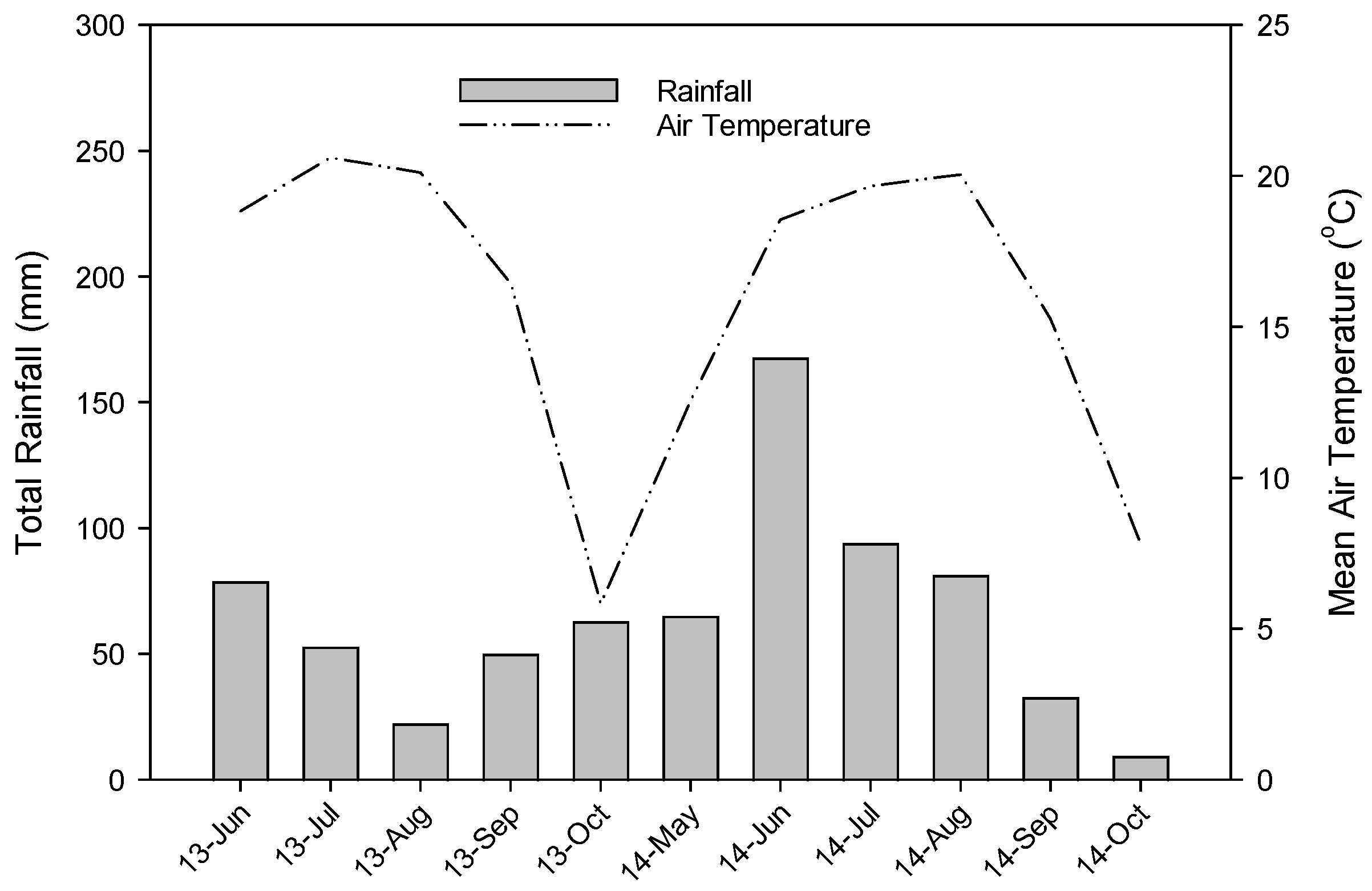
2.1. Environmental Conditions
2.2. Greenhouse Gas Analysis
2.3. Turfgrass Color and Quality
2.4. Statistical Analysis
3. Results and Discussion
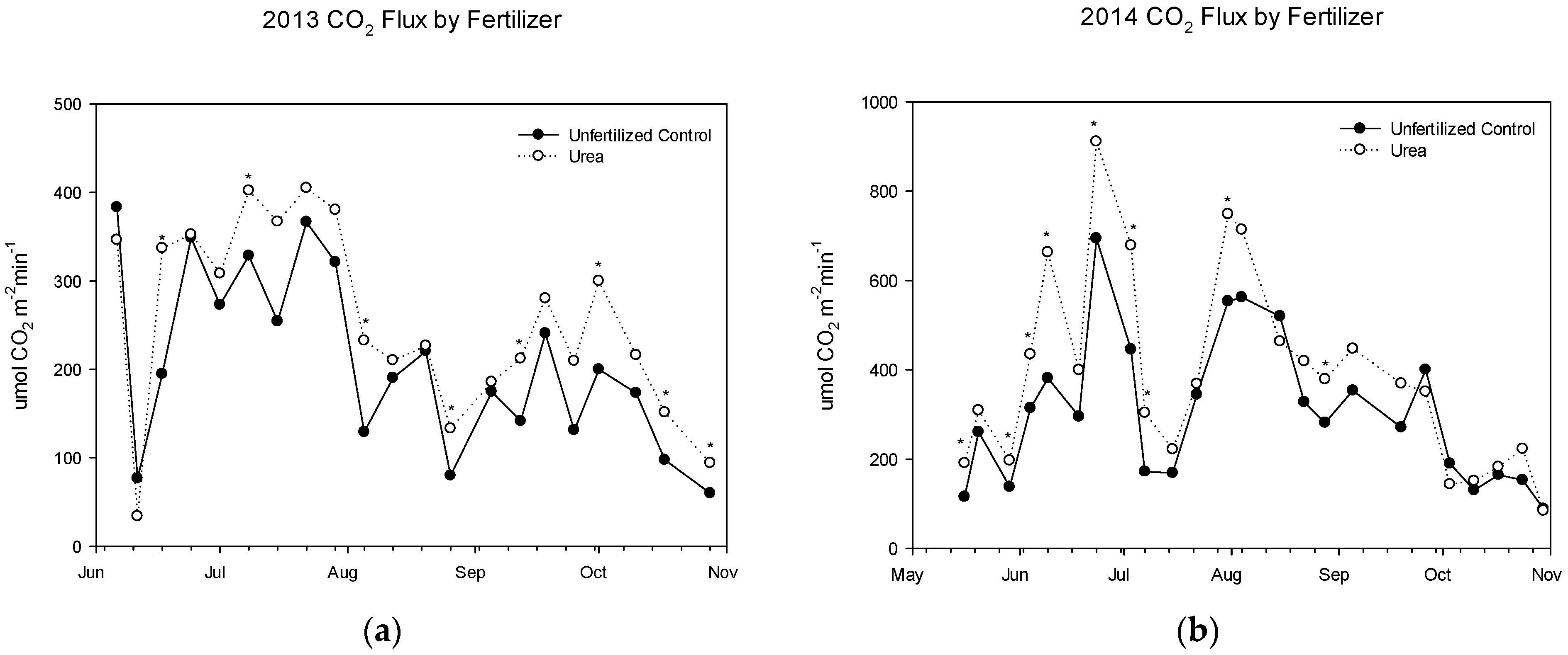
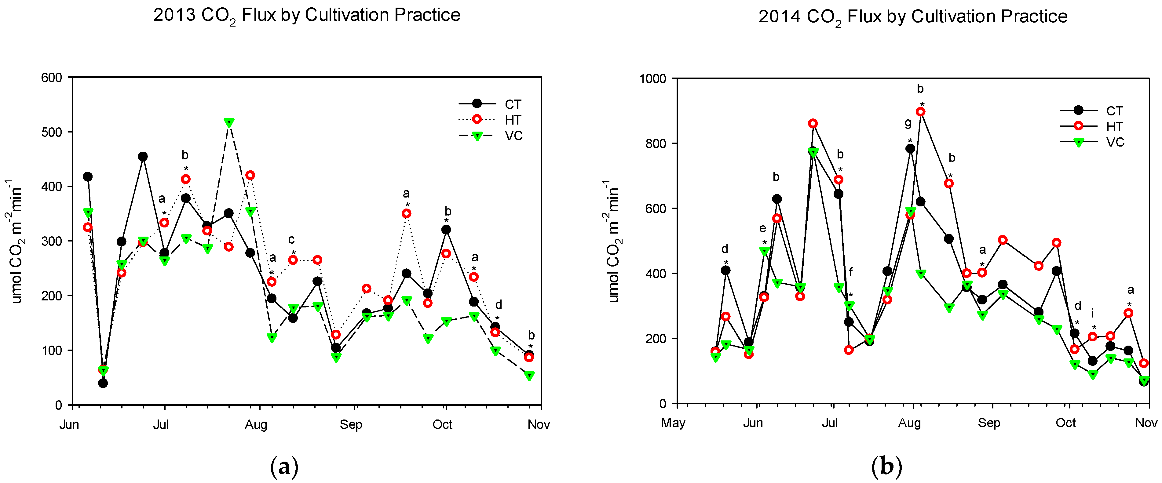
3.1. CO2 Emissions
3.2. CH4 Emissions
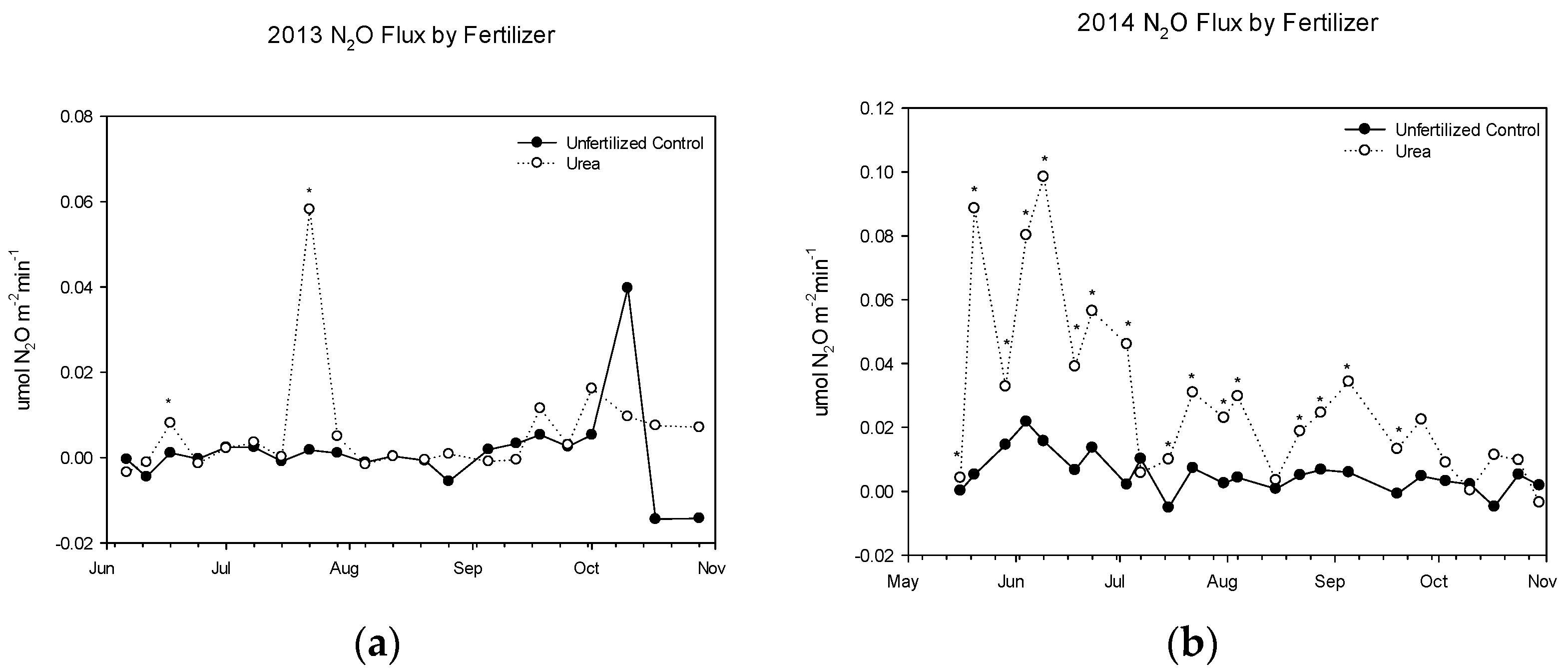
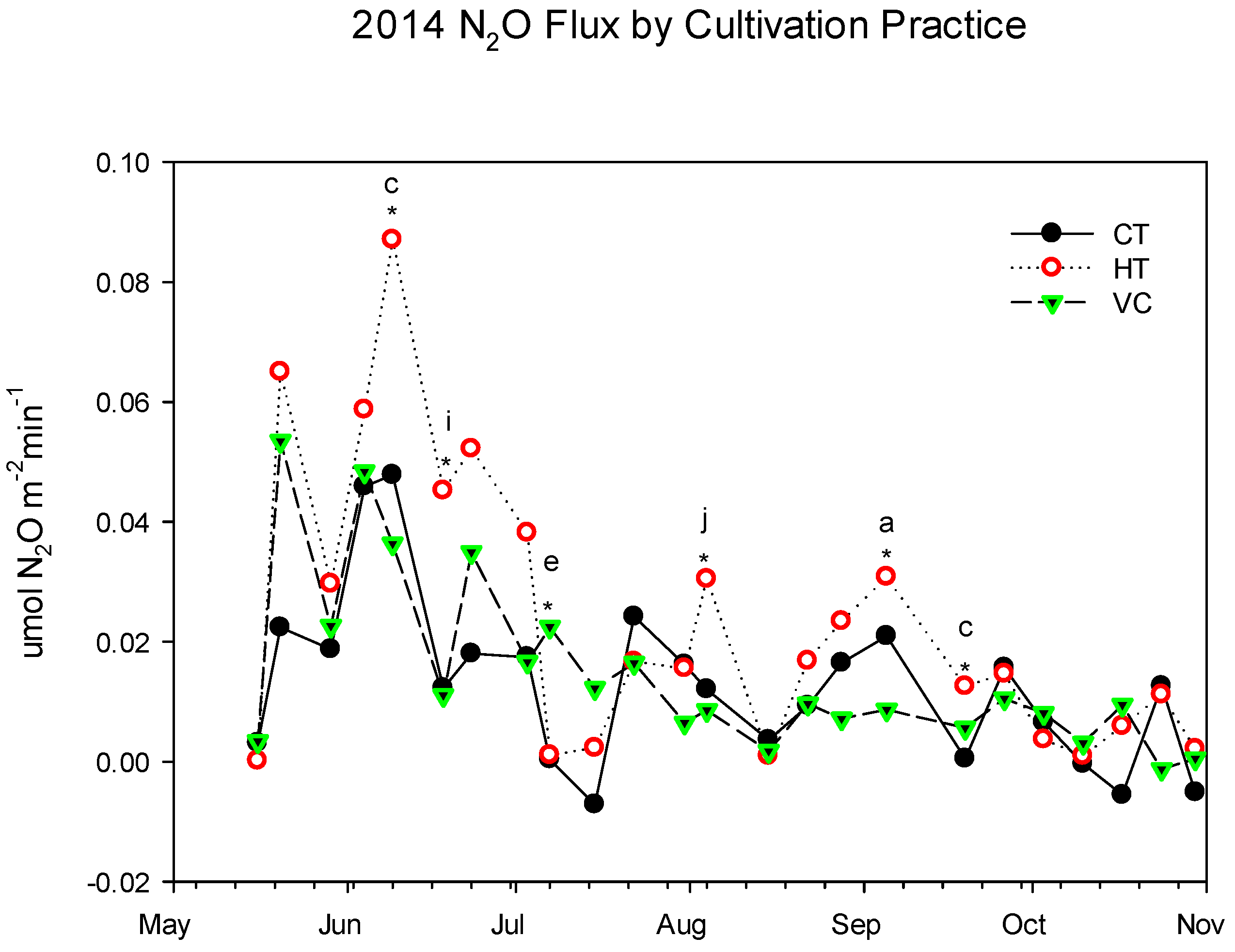
3.3. N2O Emissions
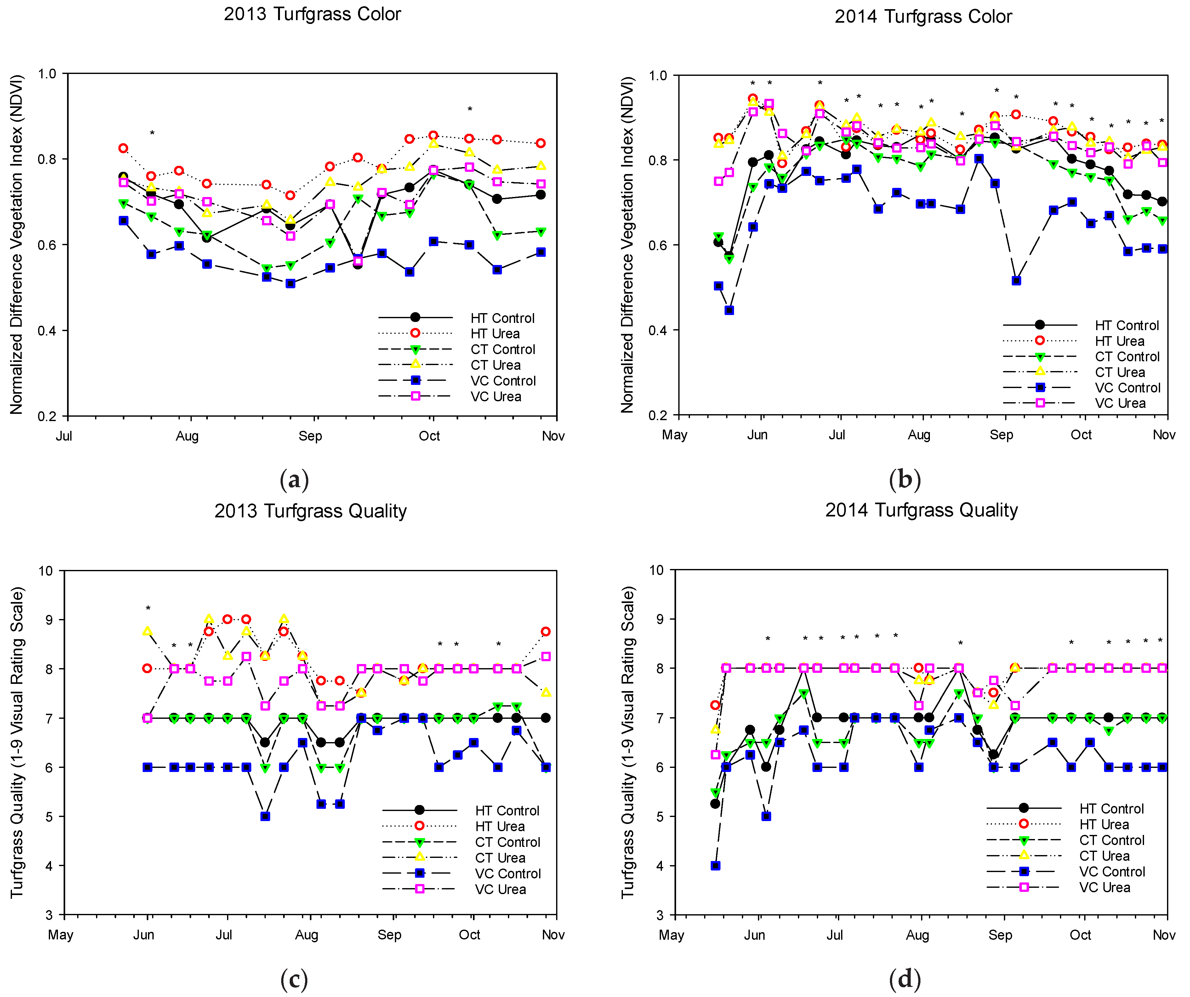
3.4. Turfgrass Color and Quality
4. Conclusions
Author Contributions
Funding
Data Availability Statement
Acknowledgments
Conflicts of Interest
References
- USEPA. Inventory of U.S. Greenhouse Gas Emissions and Sinks: 1990–2021. Available online: https://www.epa.gov/ghgemissions/inventory-us-greenhouse-gas-emissions-and-sinks-1990-2021 (accessed on 16 May 2023).
- Milesi, C.; Running, S.W.; Elvidge, C.D.; Dietz, J.B.; Tuttle, B.T.; Nemani, R.R. Mapping and Modeling the Biogeochemical Cycling of Turf Grasses in the United States. Environ. Manag. 2005, 36, 426–438. [Google Scholar] [CrossRef] [PubMed]
- Walker, K.S.; Bigelow, C.A.; Smith, D.R.; Van Scoyoc, G.E.; Reicher, Z.J. Aboveground Responses of Cool-Season Lawn Species to Nitrogen Rates and Application Timings. Crop Sci. 2007, 47, 1225–1236. [Google Scholar] [CrossRef]
- Townsend-Small, A.; Czimczik, C.I. Carbon Sequestration and Greenhouse Gas Emissions in Urban Turf. Geophys. Res. Lett. 2010, 37, 41675. [Google Scholar] [CrossRef]
- Braun, R.C.; Bremer, D.J. Carbon Sequestration in Zoysiagrass Turf under Different Irrigation and Fertilization Management Regimes. Agrosystems Geosci. Environ. 2019, 2, 180060. [Google Scholar] [CrossRef]
- Law, Q.D.; Patton, A.J. Biogeochemical Cycling of Carbon and Nitrogen in Cool-Season Turfgrass Systems. Urban For. Urban Green. 2017, 26, 158–162. [Google Scholar] [CrossRef]
- Qian, Y.; Follett, R.F.; Kimble, J.M. Soil Organic Carbon Input from Urban Turfgrasses. Soil Sci. Soc. Am. J. 2010, 74, 366–371. [Google Scholar] [CrossRef]
- Qian, Y.; Follett, R.F. Assessing Soil Carbon Sequestration in Turfgrass Systems Using Long-Term Soil Testing Data. Agron. J. 2002, 94, 930–935. [Google Scholar] [CrossRef]
- Wang, R.; Mattox, C.M.; Phillips, C.L.; Kowalewski, A.R. Carbon Sequestration in Turfgrass–Soil Systems. Plants 2022, 11, 2478. [Google Scholar] [CrossRef] [PubMed]
- Bartlett, M.D.; James, I.T. A Model of Greenhouse Gas Emissions from the Management of Turf on Two Golf Courses. Sci. Total Environ. 2011, 409, 1357–1367. [Google Scholar] [CrossRef]
- Braun, R.C.; Straw, C.M.; Soldat, D.J.; Bekken, M.A.H.; Patton, A.J.; Lonsdorf, E.V.; Horgan, B.P. Strategies for Reducing Inputs and Emissions in Turfgrass Systems. Crop Forage Turfgrass Manag. 2023, 9, e20218. [Google Scholar] [CrossRef]
- Chapman, K.E.; Walker, K.S. The Effects of Fertilizer Sources and Site Location on Greenhouse Gas Emissions from Creeping Bentgrass Putting Greens and Kentucky Bluegrass Roughs. Grasses 2023, 2, 78–97. [Google Scholar] [CrossRef]
- Braun, R.C.; Bremer, D.J. Nitrous Oxide Emissions from Turfgrass Receiving Different Irrigation Amounts and Nitrogen Fertilizer Forms. Crop Sci. 2018, 58, 1762–1775. [Google Scholar] [CrossRef]
- Law, Q.D.; Trappe, J.M.; Braun, R.C.; Patton, A.J. Greenhouse Gas Fluxes from Turfgrass Systems: Species, Growth Rate, Clipping Management, and Environmental Effects; Wiley: Hoboken, NJ, USA, 2021. [Google Scholar]
- Zhang, Y.; Qian, Y.; Bremer, D.J.; Kaye, J.P. Simulation of Nitrous Oxide Emissions and Estimation of Global Warming Potential in Turfgrass Systems Using the DAYCENT Model. J. Environ. Qual. 2013, 42, 1100–1108. [Google Scholar] [CrossRef] [PubMed]
- Bremer, D.J. Nitrous Oxide Fluxes in Turfgrass. J. Environ. Qual. 2006, 35, 1678–1685. [Google Scholar] [CrossRef] [PubMed]
- Gillette, K.L.; Qian, Y.; Follett, R.F.; Del Grosso, S. Nitrous Oxide Emissions from a Golf Course Fairway and Rough after Application of Different Nitrogen Fertilizers. J. Environ. Qual. 2016, 45, 1788–1795. [Google Scholar] [CrossRef] [PubMed]
- Kaye, J.P.; Burke, I.C.; Mosier, A.R.; Guerschman, J.P. Methane and Nitrous Oxide Fluxes from Urban Soils to the Atmosphere. Ecol. Appl. 2004, 14, 975–981. [Google Scholar] [CrossRef]
- Townsend-Small, A.; Pataki, D.E.; Czimczik, C.I.; Tyler, S.C. Nitrous Oxide Emissions and Isotopic Composition in Urban and Agricultural Systems in Southern California. J. Geophys. Res. Biogeosci. 2011, 116, 1494. [Google Scholar] [CrossRef]
- van Delden, L.; Rowlings, D.W.; Scheer, C.; Grace, P.R. Urbanisation-Related Land Use Change from Forest and Pasture into Turf Grass Modifies Soil Nitrogen Cycling and Increases N2O Emissions. Biogeosciences 2016, 13, 6095–6106. [Google Scholar] [CrossRef]
- Riches, D.; Porter, I.; Dingle, G.; Gendall, A.; Grover, S. Soil Greenhouse Gas Emissions from Australian Sports Fields. Sci. Total Environ. 2020, 707, 134420. [Google Scholar] [CrossRef]
- Walker II, E.G.; Walker, K.S. Using Agronomic Data to Minimize the Impact of Field Conditions on Player Injuries and Enhance the Development of a Risk Management Plan. J. Sports Anal. 2022, 8, 103–114. [Google Scholar] [CrossRef]
- Puhalla, J.; Krans, J.; Goatley, M. Sports Fields: Design, Construction and Maintenance; John Wiley & Sons: Hoboken, NJ, USA, 2010. [Google Scholar]
- McCarty, L.B. Best Golf Course Management Practices, 3rd ed.; Prentice Hall: Saddle River, NJ, USA, 2011. [Google Scholar]
- Reicosky, D.C.; Lindstrom, M.J. Fall Tillage Method: Effect on Short-Term Carbon Dioxide Flux from Soil. Agron. J. 1993, 85, 1237–1243. [Google Scholar] [CrossRef]
- Reicosky, D.C.; Kemper, W.D.; Langdale, G.W.; Douglas, C.L.; Rasmussen, P.E. Soil Organic Matter Changes Resulting from Tillage and Biomass Production. J. Soil Water Conserv. 1995, 50, 253–261. [Google Scholar]
- Reicosky, D.C.; Dugas, W.A.; Torbert, H.A. Tillage-Induced Soil Carbon Dioxide Loss from Different Cropping Systems. Soil Tillage Res. 1997, 41, 105–118. [Google Scholar] [CrossRef]
- Smith, K.; Watts, D.; Way, T.; Torbert, H.; Prior, S. Impact of Tillage and Fertilizer Application Method on Gas Emissions in a Corn Cropping System. Pedosphere 2012, 22, 604–615. [Google Scholar] [CrossRef]
- Kessavalou, A.; Mosier, A.R.; Doran, J.W.; Drijber, R.A.; Lyon, D.J.; Heinemeyer, O. Fluxes of Carbon Dioxide, Nitrous Oxide, and Methane in Grass Sod and Winter Wheat-Fallow Tillage Management. J. Environ. Qual. 1998, 27, 1094–1104. [Google Scholar] [CrossRef]
- GRACEnet Sampling Protocols: USDA ARS. Available online: https://www.ars.usda.gov/natural-resources-and-sustainable-agricultural-systems/soil-and-air/docs/gracenet-sampling-protocols/ (accessed on 12 October 2022).
- Mosier, A.R. Exchange of Gaseous Nitrogen Compounds between Agricultural Systems and the Atmosphere. Plant Soil 2001, 228, 17–27. [Google Scholar] [CrossRef]
- Morris, K.N.; Shearman, R.C. NTEP Turfgrass Evaluation Guidelines. In Proceedings of the NTEP Turfgrass Evaluation Workshop, Beltsville, MD, USA, 17 October 1998; pp. 1–5. [Google Scholar]
- Bell, G.E.; Martin, D.L.; Wiese, S.G.; Dobson, D.D.; Smith, M.W.; Stone, M.L.; Solie, J.B. Vehicle-Mounted Optical Sensing: An Objective Means for Evaluating Turf Quality. Crop Sci. 2002, 42, 197–201. [Google Scholar] [CrossRef] [PubMed]
- Bremer, D.J.; Lee, H.; Su, K.; Keeley, S.J. Relationships between Normalized Difference Vegetation Index and Visual Quality in Cool-Season Turfgrass: II. Factors Affecting NDVI and Its Component Reflectances. Crop Sci. 2011, 51, 2219–2227. [Google Scholar] [CrossRef]
- Jiang, Y.; Carrow, R.N. Assessment of Narrow-Band Canopy Spectral Reflectance and Turfgrass Performance under Drought Stress. HortScience 2005, 40, 242–245. [Google Scholar] [CrossRef]
- Jiang, Y.; Carrow, R.N. Broadband Spectral Reflectance Models of Turfgrass Species and Cultivars to Drought Stress. Crop Sci. 2007, 47, 1611–1618. [Google Scholar] [CrossRef]
- Lee, H.; Bremer, D.J.; Su, K.; Keeley, S.J. Relationships between Normalized Difference Vegetation Index and Visual Quality in Turfgrasses: Effects of Mowing Height. Crop Sci. 2011, 51, 323–332. [Google Scholar] [CrossRef]
- Trenholm, L.E.; Carrow, R.N.; Duncan, R.R. Relationship of Multispectral Radiometry Data to Qualitative Data in Turfgrass Research. Crop Sci. 1999, 39, 11183X003900030025x. [Google Scholar] [CrossRef]
- Leinauer, B.; VanLeeuwen, D.M.; Serena, M.; Schiavon, M.; Sevostianova, E. Digital Image Analysis and Spectral Reflectance to Determine Turfgrass Quality. Agron. J. 2014, 106, 1787–1794. [Google Scholar] [CrossRef]
- SAS/STAT 9.1: User’s Guide; Clark, V., SAS Institute, Eds.; SAS Pub: Cary, NC, USA, 2004; ISBN 978-1-59047-243-9. [Google Scholar]
- Henry, F.; Nguyen, C.; Paterson, E.; Sim, A.; Robin, C. How Does Nitrogen Availability Alter Rhizodeposition in Lolium Multiflorum Lam. during Vegetative Growth? Plant Soil 2005, 269, 181–191. [Google Scholar] [CrossRef]
- Kaye, J.P.; Hart, S.C. Competition for Nitrogen between Plants and Soil Microorganisms. Trends Ecol. Evol. 1997, 12, 139–143. [Google Scholar] [CrossRef]
- Rice, P.J.; Horgan, B.P.; Hamlin, J.L. Evaluation of Individual and Combined Management Practices to Reduce the Off-Site Transport of Pesticides from Golf Course Turf. Sci. Total Environ. 2017, 583, 72–80. [Google Scholar] [CrossRef]
- Rice, P.J.; Horgan, B.P. Evaluation of Nitrogen and Phosphorus Transport with Runoff from Fairway Turf Managed with Hollow Tine Core Cultivation and Verticutting. Sci. Total Environ. 2013, 456, 61–68. [Google Scholar] [CrossRef] [PubMed]
- Christians, N.E.; Patton, A.J.; Law, Q.D. Fundamentals of Turfgrass Management; John Wiley & Sons: Hoboken, NJ, USA, 2016. [Google Scholar]
- Myrold, D.D.; Tiedje, J.M. Diffusional Constraints on Denitrification in Soil. Soil Sci. Soc. Am. J. 1985, 49, 651–657. [Google Scholar] [CrossRef]
- Myrold, D.D.; Tiedje, J.M. Establishment of Denitrification Capacity in Soil: Effects of Carbon, Nitrate and Moisture. Soil Biol. Biochem. 1985, 17, 819–822. [Google Scholar] [CrossRef]
- Tiedje, J.M.; Sexstone, A.J.; Myrold, D.D.; Robinson, J.A. Denitrification: Ecological Niches, Competition and Survival. Antonie Van Leeuwenhoek 1983, 48, 569–583. [Google Scholar] [CrossRef]
- Nektarios, P.A.; Petrovic, A.M.; Steenhuis, T.S. Preferential flow in simulated greenhouse golf putting green profiles as affected by aeration and two soil moisture regimes. Soil Sci. 2007, 172, 108. [Google Scholar] [CrossRef]

| CO2 | N2O | CH4 | |||||
|---|---|---|---|---|---|---|---|
| Year | Treatment | Mean | Median | Mean | Median | Mean | Median |
| g CO2-C m−2 h−1 | µg N2O-N m−2 h−1 | µg CH4-C m−2 h−1 | |||||
| 2013 | |||||||
| Cultivation | |||||||
| CT | 0.27 ab | 0.21 | 3.63 | 1.64 | −3.24 | −3.53 | |
| HT | 0.28 a | 0.26 | 3.05 | 2.89 | −3.38 | −2.52 | |
| VC | 0.24 b | 0.21 | 7.99 | 1.27 | 7.92 | −0.864 | |
| Fertilizer | |||||||
| Urea | 0.29 A | 0.26 | 8.13 | 2.92 | 0.201 | −1.30 | |
| UC | 0.24 B | 0.19 | 1.65 | 1.26 | 0.864 | −2.59 | |
| ANOVA | |||||||
| Source of Variation | df | df | df | ||||
| Cultivation | 2 | * | 2 | NS | 2 | NS | |
| Fertilizer | 1 | *** | 1 | NS | 1 | NS | |
| Cultivation × Fertilizer | 2 | NS | 2 | NS | 2 | NS | |
| 2014 | |||||||
| Cultivation | |||||||
| HT | 0.44 a | 0.35 | 32.5 a | 14.3 | 10.8 ab | 0.30 | |
| VC | 0.33 b | 0.28 | 20.5 b | 8.95 | 20.1 a | 2.90 | |
| CT | 0.41 a | 0.36 | 14.6 b | 8.4 | 2.66 b | −1.94 | |
| Fertilizer | |||||||
| Urea | 0.44 A | 0.39 | 39.6 A | 21.8 | 9.36 | −1.58 | |
| UC | 0.35 B | 0.29 | 7.41 B | 4.74 | 13.0 | 1.22 | |
| ANOVA | |||||||
| Source of Variation | df | df | df | ||||
| Cultivation | 2 | *** | 2 | ** | 2 | * | |
| Fertilizer | 1 | *** | 1 | *** | 1 | NS | |
| Cultivation × Fertilizer | 2 | NS | 2 | NS | 2 | NS | |
| Year | Treatment | Mean | Median |
|---|---|---|---|
| 2013 | |||
| Cultivation | |||
| HT | 13.6 a | 12.8 | |
| VC | 12.2 b | 10.5 | |
| CT | 11.9 b | 10.4 | |
| Fertilizer | |||
| Urea | 13.1 | 10.7 | |
| UC | 12.1 | 11.8 | |
| ANOVA | |||
| Source of Variation | df | ||
| Cultivation | 2 | * | |
| Fertilizer | 1 | NS | |
| Cultivation × Fertilizer | 2 | NS | |
| 2014 | |||
| Cultivation | |||
| HT | 19.6 | 17.6 | |
| VC | 20.2 | 17.8 | |
| CT | 19.6 | 17.3 | |
| Fertilizer | |||
| Urea | 18.7 B | 18.9 | |
| UC | 20.7 A | 20.7 | |
| ANOVA | |||
| Source of Variation | df | ||
| Cultivation | 2 | NS | |
| Fertilizer | 1 | * | |
| Cultivation × Fertilizer | 2 | NS |
| Treatment | Turfgrass Color | Turfgrass Quality | |||
|---|---|---|---|---|---|
| 2013 | 2014 | 2013 | 2014 | ||
| NDVI | Visual Rating (1–9 Scale) | ||||
| Cultivation | |||||
| HT | 0.75 A | 0.82 A | 7.5 A | 7.4 A | |
| VC | 0.64 C | 0.76 B | 7.0 B | 7.0 B | |
| CT | 0.70 B | 0.82 B | 7.4 A | 7.3 A | |
| Fertilizer | |||||
| Urea | 0.75 a | 0.86 a | 8.0 a | 7.9 a | |
| UC | 0.64 b | 0.74 b | 6.6 b | 6.6 b | |
| ANOVA | |||||
| Source of Variation | |||||
| Cultivation | *** | *** | *** | *** | |
| Fertilizer | *** | *** | *** | *** | |
| Cultivation × Fertilizer | NS | *** | ** | *** | |
Disclaimer/Publisher’s Note: The statements, opinions and data contained in all publications are solely those of the individual author(s) and contributor(s) and not of MDPI and/or the editor(s). MDPI and/or the editor(s) disclaim responsibility for any injury to people or property resulting from any ideas, methods, instructions or products referred to in the content. |
© 2024 by the authors. Licensee MDPI, Basel, Switzerland. This article is an open access article distributed under the terms and conditions of the Creative Commons Attribution (CC BY) license (https://creativecommons.org/licenses/by/4.0/).
Share and Cite
Walker, K.S.; Chapman, K.E. The Effects of Cultivation Practices and Fertilizer Use on the Mitigation of Greenhouse Gas Emissions from Kentucky Bluegrass Athletic Fields. Horticulturae 2024, 10, 869. https://doi.org/10.3390/horticulturae10080869
Walker KS, Chapman KE. The Effects of Cultivation Practices and Fertilizer Use on the Mitigation of Greenhouse Gas Emissions from Kentucky Bluegrass Athletic Fields. Horticulturae. 2024; 10(8):869. https://doi.org/10.3390/horticulturae10080869
Chicago/Turabian StyleWalker, Kristina S., and Katy E. Chapman. 2024. "The Effects of Cultivation Practices and Fertilizer Use on the Mitigation of Greenhouse Gas Emissions from Kentucky Bluegrass Athletic Fields" Horticulturae 10, no. 8: 869. https://doi.org/10.3390/horticulturae10080869
APA StyleWalker, K. S., & Chapman, K. E. (2024). The Effects of Cultivation Practices and Fertilizer Use on the Mitigation of Greenhouse Gas Emissions from Kentucky Bluegrass Athletic Fields. Horticulturae, 10(8), 869. https://doi.org/10.3390/horticulturae10080869