Estimating the Grape Basal Crop Coefficient in the Subhumid Region of Northwest China Based on Multispectral Remote Sensing by Unmanned Aerial Vehicle

Abstract

How to quickly and accurately obtain the basal crop coefficient is the key to estimating evapotranspiration in sparse vegetation. To enhance the accuracy of vineyard evapotranspiration estimation in the subhumid region of Northwest China, this study utilized the actual evapotranspiration (ET_c) measured by the Bowen ratio system as the reference standard. The reference crop evapotranspiration (ET_o) was calculated using the Penman formula, and the grape crop coefficient (K_c) was subsequently derived. The FAO-56 dual crop coefficient method was then employed to determine the soil evaporation coefficient (K_e) and the water stress coefficient (K_s), leading to the acquisition of the basal crop coefficient (K_cb). Concurrently, multispectral remote sensing images captured by unmanned aerial vehicle (UAV) were used to gather grape spectral data, from which the reflectance of multiple bands was extracted to compute four vegetation indices: the Normalized Difference Vegetation Index (NDVI), the Soil-Adjusted Vegetation Index (SAVI), the Ratio Vegetation Index (RVI), and the Difference Vegetation Index (DVI). Relationship models between the grape basal crop coefficient (K_cb) and these vegetation indices were established using univariate linear regression, polynomial regression, and multiple linear regression. These models were then used to estimate vineyard evapotranspiration and validate the accuracy of the UAV multispectral remote sensing in estimating the grape K_cb. The results indicated that: (1) The growth stage, type of vegetation index, and modeling method were three significant factors influencing the fitting accuracies of the relationship models between the grape basal crop coefficient (K_cb) and vegetation indices. These model fitting accuracies had a notable impact on the estimation accuracies of evapotranspiration. (2) The application of UAV-based multispectral remote sensing to estimate the grape basal crop coefficient in the subhumid region of Northwest China was feasible. Compared to the K_cb values recommended by the FAO-56, the K_cb values derived from the UAV data improved the estimation accuracies of evapotranspiration by more than 11% in 2021 and 13% in 2022.

1. Introduction

Crop evapotranspiration mainly includes soil evaporation and vegetation transpiration. It is an important way for crops to exchange water with the atmosphere [1]. As an important part of the global water cycle and surface energy balance, crop evapotranspiration has an important impact on crop growth and yield. Crop evapotranspiration is the basis for determining a rational irrigation regime, which encompasses the determination of optimal irrigation timing, irrigation amount, and irrigation methods, among other factors [2,3]. China is the world’s largest producer and consumer of table grape. The grape planting area is stable at more than 660,000 hectares [4] with considerable economic value. As one of the important producing areas of table grape in China, Shaanxi has significantly increased its viticulture area and yield in recent years [5]. Proper water supply is one of the basic conditions to ensure high quality and high yield of grape. Water deficit or excess of vineyards will not only affect the yield and quality of grape in the current season but also affect the grape growth and development in the next season, even shortening the growth years of the vineyards. These all increase the complexity and particularity of vineyard water management [6]. Accurate estimation of evapotranspiration during the grape growth period is crucial, as it underpins the determination of a rational irrigation regime necessary to fulfill the water requirements for optimal grape production.

The commonly used methods to obtain crop evapotranspiration are divided into two categories: measurement methods and estimation methods. Measurement methods mainly include the Eddy covariance method, the Bowen ratio method, the Lysimeter method, and the isotope method (by analyzing the isotopic composition of water vapor, such as hydrogen and oxygen isotopes, the contributions of evaporation and transpiration to the overall evapotranspiration process can be distinguished [7]). Scholars from various countries [8,9,10,11,12] have verified the applicability and accuracy of obtaining the crop’s actual evapotranspiration by using the above methods. However, most of these methods are technically complex, high cost, and high maintenance costs, with these instruments potentially reaching tens of thousands of dollars. Individual methods require a sufficiently large, flat, and uniform underlying surface; otherwise, it is difficult to achieve a certain accuracy.

Estimation methods for evapotranspiration can be broadly categorized into direct estimation methods and indirect estimation methods. Direct estimation methods mainly encompass single-source models and multi-source models. Among the single-source models, the P-M model is well supported by theory. However, it overlooks the disparities in water and heat characteristics between the canopy and soil, leading to significant deviations in the estimation of evapotranspiration for sparse vegetation. The multi-source models, while more complex in mechanism, face challenges in parameter acquisition and are computationally intensive, often resulting in “over-fitting” and thus limited practical applicability. The crop coefficient method stands as the most prevalent indirect estimation technique. Notably, the dual-crop coefficient method proposed by FAO-56 is straightforward and has gained widespread adoption [13,14,15,16]. Despite its empirical basis and broad applicability, it cannot provide precise evapotranspiration estimates for all regions and crops.

The crop coefficients in the dual crop coefficient method must be adjusted according to the growth condition of crops and the external environment (water stress, meteorological conditions) to accurately estimate the actual evapotranspiration. It is difficult to carry out ground monitoring and adjust crop coefficient curves at any time. In such cases, employing remote sensing technology to estimate crop coefficients would be more convenient. In recent years, remote sensing technology has risen rapidly in China. It has been gradually applied in different research fields and reached a high level of development. Particularly, the application of remote sensing for crop coefficient estimation has overcome many limitations of other existing research methods [17,18]. In contrast, remote sensing is relatively more affordable. Remote sensing applications are mainly divided into satellite remote sensing and low-altitude airborne remote sensing. Satellite remote sensing is the earliest development and has reached a high degree of maturity, but its data preprocessing results are easily affected by atmospheric conditions. It is difficult to obtain reliable and consistent data. The low-altitude UAV remote sensing not only overcomes the problems of satellite remote sensing, such as being greatly affected by atmospheric conditions, long revisit periods, and unmatched spatiotemporal resolution, but also avoids the disadvantages of time-consuming and strenuous monitoring of crop growth information on the ground. It highlights low cost, flexibility, real-time image acquisition, high timeliness, and high spatiotemporal resolution [19,20]. These advantages make UAVs particularly suitable for small-scale and research applications, where detailed and timely data are crucial.

UAV remote sensing technology can better estimate the daily crop coefficient to meet the demand for estimating the daily crop evapotranspiration at the field scale [21]. Marcialpablo et al. [22] demonstrated that images with ground objects removed based on unmanned aerial vehicle (UAV) spectral remote sensing can estimate the K_c of corn with relatively high precision, where K_c fits best with NDVI at 80,000 plants per hectare. Zhang Yu [23] used UAV multispectral remote sensing technology in conjunction with ground monitoring to establish a relationship model between the crop coefficient K_c with vegetation indices and argued for its feasibility. Han Wenting et al. [24] used UAV multispectral remote sensing technology to obtain six vegetation indices and established their relationship models with the crop coefficient of field corn under different water stress conditions during various growth stages, showing that the vegetation index SR had the best correlation with the crop coefficient under sufficient irrigation conditions during the rapid growth stage and under water stress conditions during the late growth stage. Shao et al. [25] combined UAV multispectral remote sensing technology with the random forest algorithm to obtain high-resolution spatial distribution maps of corn K_c values under different irrigation conditions. Gautam et al. [26] used UAV-mounted multispectral sensors to extract spectral and structural characteristics of Cabernet Sauvignon grapes and modeled K_c through multiple linear regression and machine learning methods. The results showed that combining canopy structural features with spectral features can improve model applicability. Among all the prediction models, the random forest predicted the highest precision of K_c.

To date, research on crop coefficient (K_c) estimation in China has predominantly concentrated on economic and field crops. Studies focusing on perennial fruit trees, characterized by well-developed root systems and sparse planting patterns, are notably scarce. Given the significant individual variability among grapevines, precise water and fertilizer management is essential, yet such research is seldom documented. Unlike densely planted crops, which exhibit minimal soil evaporation, both vegetation transpiration and soil evaporation contribute significantly to the total evapotranspiration of grapefruit trees and can be considered as two relatively independent components. Therefore, it is imperative to conduct separate investigations into their basal crop coefficient (K_cb). Currently, research on estimating the crop coefficient of sparse vegetation at the field scale using UAV remote sensing technology remains insufficient. Therefore, this study selected the vineyard located in Jundu Weier Vineyard (108°08′ E, 34°31′ N), Cui Xigou Village, Yangling District, Xianyang City, Shaanxi Province, China, as the research site for the years 2021 and 2022. The evapotranspiration (ET_c) measured by the Bowen ratio system was used as the reference standard. The reference crop evapotranspiration (ET_o) was calculated using the Penman formula, and the grape crop coefficient (K_c) was subsequently derived. The soil evaporation coefficient (K_e) and the water stress coefficient (K_s) were determined using the FAO-56 dual crop coefficient method, which facilitated the acquisition of the basal crop coefficient (K_cb). Multispectral remote sensing images captured by an unmanned aerial vehicle (UAV) were employed to gather grape spectral data, from which the reflectance of multiple bands was extracted to compute four vegetation indices. Relationship models between the grape basal crop coefficient (K_cb) and vegetation indices were established to estimate evapotranspiration in the vineyard. The accuracy of the grape K_cb retrieval using UAV multispectral remote sensing was validated by comparing the estimated evapotranspiration values with the measured values. By employing this method, we aim to enhance the accuracy of evapotranspiration estimation, thereby providing theoretical guidance and technical support for precision irrigation in this region.

2. Materials and Methods

2.1. Overview of the Study Area and Grape Phenological Stages

The experiment was conducted from April to August 2021 and 2022 in Jundu Weier Vineyard, Cui Xigou Village, Yangling District, Xianyang City, Shaanxi Province, China. The manor is located in the middle of the Guanzhong Plain in Shaanxi Province (108°08′ E, 34°31′ N), with an altitude of 524.7 m. This region is situated within the warm temperate subhumid climatic zone, characterized by distinct seasonal patterns, with cold and dry winters and hot and rainy summers [27]. Among them, the annual average temperature is 12.9 °C. The annual average evaporation is 1500 mm, and the annual average precipitation is 580 mm. The grapes in the experimental area are about 5 years old, and the name is Black Sugar Beet. The planting rows of grapes are from south to north and the row spacing is about 3 m. It is about 20 rows in total. The length of each row is about 18 m, and the spacing of vines is about 0.8 m. The vineyard is dominated by drip irrigation. The field treatment, such as irrigation and fertilization, in the experiment for 2 years is consistent with local grape production without special water and fertilizer control. According to the grape growth characteristics, its growth period was divided into four growth stages, which were the new shoot growth stage, the flowering stage, the fruit expansion stage, and the coloring maturity stage. The specific timings of each growth stage of grape over the two years are shown in

Table 1. Grape growth stage.

Growth Stage	Date of Grape Growth Stage Partition
	2021	2022
New shoot growth stage	4/12–5/15	4/8–5/12
Flowering stage	5/16–5/30	5/13–5/28
Fruit expansion stage	5/31–7/6	5/29–7/5
Coloring maturity stage	7/7–8/20	7/6–8/20

.

2.2. Meteorological Data

The meteorological data, such as net radiation R_n, wind speed W_s, wind vector W_d, air temperature T_a, relative humidity RH, water vapor pressure e, soil heat flux G, and canopy temperature T_c in the test area of this study, were automatically observed by the Bowen ratio system every 10 min all day long. Rainfall data were provided by Yangling Meteorological Station. The reference crop evapotranspiration ET_o was calculated using Penman’s formula (Equation (1)). Rainfall data and ET_o for 2021 and 2022 are shown in Figure 1.

$$E{T}_O={\displaystyle \frac{0.408\Delta (R_n-G)+\gamma \frac{900}{T+273}{u}_2(e_s-e_a)}{\Delta +\gamma (1+0.34u_2)}}$$

(1)

where ET_o is reference crop evapotranspiration, mm/d; R_n is the net radiation of crop canopy, MJ/(m²∙d); G is the soil heat flux, MJ/(m²∙d), G = 0 in daily calculation; T is the average temperature, °C; u₂ is the average wind speed at 2 m height, m/s; e_s is the saturated water vapor pressure, kPa; e_a is the actual water vapor pressure, kPa; Δ is the slope of the saturation water pressure and temperature curve, kPa/°C; and γ is the psychrometric constant.

2.3. The Bowen Ratio Energy Balance Method

The Bowen ratio energy balance method is a widely used method to estimate evapotranspiration in farmland. This method estimates the latent heat flux by measuring the temperature and humidity gradient, combined with the measurement of net radiation and ground heat flux [28]. The basic principle is the conservation of energy. The advantages are that fewer measured parameters are required and the calculation method is simple. There are no data on the aerodynamic characteristics of the evapotranspiration surface required. The latent heat flux of a large area (about 1000 m²) and small time scale (10 min) can be estimated. Based on the principle of conservation of energy, the energy balance equation represents the sum of all energy absorbed and released on the underlying surface. Its calculation equation is shown in Equation (2):

$$R_{\mathrm{n}}=\lambda ET+H+G+AD+PH+M$$

(2)

where R_n is the net radiation, W/m²; λET is the latent heat flux, W/m²; λ is the latent heat of vaporization, J/kg; ET is evapotranspiration, mm; H is sensible heat flux, W/m²; G is soil heat flux, W/m²; AD is the horizontal exchange capacity of energy, W/m²; PH is photosynthetic energy conversion, W/m²; and M is composed of energy conversion caused by plant metabolism and heat storage in plant interior and canopy, W/m².

AD can be ignored when the bottom surface is uniform and the area is large. When PH and M are too small, they can also be ignored under normal circumstances; then Equation (2) can be simplified as

$$R_n=\lambda ET+H+G$$

(3)

2.4. The Dual Crop Coefficient Method

The dual crop coefficient method requires only conventional meteorological elements and is widely used to calculate evapotranspiration for one day or longer because of its simple characteristics [29]. The calculation formula is as follows:

$$E{T}_{\mathrm{c}}=({K_{\mathrm{cb}}}^{\prime }\cdot K_{\mathrm{s}}+K_e)\cdot E{T}_{\mathrm{o}}$$

(4)

where ET_c refers to the actual crop evapotranspiration amount calculated using the dual crop coefficient method after obtaining the grape basal crop coefficient from the inversion of multispectral remote sensing data by unmanned aerial vehicle (UAV) (mm); ET_o is the reference crop evapotranspiration (mm), which was calculated by Formula (1); and K_cb’ was derived from the relationship of the K_cb-VI_s models.

K_s is the coefficient of soil water stress. In this paper, the calculation formula of K_s recommended by FAO-56 is as follows:

$$K_s=\left\{\begin{array}{l}{\displaystyle \frac{TAW-D_r}{TAW-RAW}}\\ 1.0\end{array}\right.\begin{array}{l}{D}_{\mathrm{r}}>R_{AW}\\ D_r\le R_{AW}\end{array}$$

(5)

$$TAW=10\rho b\cdot Z_r({\theta }_{fc}-{\theta }_{wp})$$

(6)

$$D_r=10\rho b\cdot Z_r({\theta }_{fc}-\theta )$$

(7)

$$RAW=p\cdot TAW$$

(8)

where TAW is the total soil effective water storage in the main root layer of crops (mm). RAW is the root zone soil water storage (mm) that is easily utilized by crop roots. D_r is the average soil water deficit of the crop root zone during the calculation period. When the calculation period is short, the soil water deficit at the beginning of the period can be used to replace (mm). ρb is soil bulk density (g·cm⁻³); Z_r is the main active layer depth (cm) of crop roots. θ is the average soil moisture content in the root layer of early crops (m³m⁻³). θ_fc and θ_wp are the field capacity and wilting point capacity of the root zone (m³m⁻³), respectively. p is the ratio of soil water storage easily absorbed by crop roots to the total available soil water storage in the root zone, generally ranging from 0 to 1.

K_e is the evaporation coefficient of surface soil. In this paper, the calculation formula of K_e recommended by FAO-56 is as follows

$$K_{\mathrm{e}}=K_r(K_{c\max }-K_{cb})\le f_{ew}{K}_{c\max }$$

(9)

where K_c,max is the maximum crop coefficient after rainfall or irrigation; K_r is the soil evaporation attenuation coefficient determined by the cumulative evaporation depth. When the soil surface is relatively moist (rainfall 1~2 d), K_r is 1. After the rainfall (3~5 d), the surface wetness decreases, and the K_r value is 0.7. After the rainfall (6~8 d), the surface moisture continued to decrease, and the K_r value was 0.2. When the surface water used for evaporation is completely exhausted, the K_r value is 0. f_ew is the proportion of soil with inter-plant evaporation in the total soil.

K_cb is the basal crop coefficient and the calculation formula in this paper is

$$K_{\mathrm{cb}}={\displaystyle \frac{\frac{ET}{E{T}_{\mathrm{o}}}-K_e}{K_{\mathrm{s}}}}$$

(10)

where ET is the actual crop evapotranspiration (mm), the measured values in this paper were provided by the Bowen ratio system; K_s and K_e can be obtained by Formulas (5) and (9), respectively.

2.5. Multispectral Image Acquisition and Preprocessing

The four-rotor Phantom4 UAV of Dajiang Innovation Technology Co.(Shenzhen, China), Ltd. was used as the data acquisition platform. The UAV is an integrated multispectral imaging system with a multispectral camera with six image sensors. One of the color sensors is for visible light (RGB) imaging, and the other five monochromatic sensors are used for multispectral imaging in the blue (B, 450 nm ± 16 nm), green (G, 560 nm ± 16 nm), red (R, 650 nm ± 16 nm), red-edge (RE, 730 nm ± 16 nm), and near-infrared (NIR, 840 nm ± 26 nm) bands. The test set UAV route has a relative navigation height of 30 m, a course overlap rate of 80%, a side overlap rate of 70%, and a ground resolution of 1.6 cm. The RGB and multispectral images of the study area can be obtained synchronously during the operation. The multispectral remote sensing images of UAV were collected during clear sky conditions with stable sunlight. In 2021, we obtained a total of 60 valid flight data sets, and in 2022, we obtained 48 sets. The obtained multispectral images were checked and imported into DJI Terra software without error. The field scene was reconstructed in two dimensions, and the orthophoto images based on a single band were obtained. The single-band images were imported into ENVI5.3 software for band merging, and finally, the vineyard multispectral images after multi-band fusion were obtained. The orthophotos of the four growth stages of grape after band fusion are shown in Figure 2. After removing the background of the multispectral image with MATLAB 2016a, the normalized difference vegetation index was utilized to distinguish grape plants from other ground objects and eliminate the soil background, and different band reflectances were extracted to calculate various vegetation indices.

2.6. Vegetation Index Calculation

In this paper, eight kinds of commonly used vegetation indices were used for preliminary calculation. Among them, NDVI can detect vegetation growth state, vegetation coverage, and eliminate some radiation errors. SAVI increases the soil conditioning coefficient and decreases the sensitivity of NDVI to soil background. RVI is a sensitive indicator parameter of green vegetation, which is more sensitive to high vegetation cover areas and has the best correlation with biomass. DVI is sensitive to the change in soil background. EVI is applicable under conditions of vegetation index saturation. VARI can mitigate the impacts caused by differences in illumination and atmospheric effects. GNDVI is sensitive to changes in crop pigments. ARVI can reduce the dependence of vegetation indices on atmospheric properties. The formula for calculating the vegetation index can be found in

Table 2. Calculation formula of vegetation index.

Vegetation Index	Computational Formula	Reference
NDVI	$NDVI={\displaystyle \frac{R_{Nir}-R_{\mathrm{Re}d}}{R_{Nir}+R_{\mathrm{Re}d}}}$	[30]
SAVI	$SAVI=1.5\times {\displaystyle \frac{R_{Nir}-R_{\mathrm{Re}d}}{R_{Nir}+R_{\mathrm{Re}d}+0.5}}$	[31]
RVI	$RVI={\displaystyle \frac{R_{Nir}}{R_{\mathrm{Re}d}}}$	[32]
DVI	$DVI=R_{Nir}-R_{\mathrm{Re}d}$	[33]
EVI	$EVI=2.5\times {\displaystyle \frac{R_{Nir}-R_{\mathrm{Re}d}}{R_{Nir}+6R_{\mathrm{Re}d}-R_{Blue}+1}}$	[34]
VARI	$VARI={\displaystyle \frac{R_{Green}-R_{\mathrm{Re}d}}{R_{Green}+R_{\mathrm{Re}d}-R_{Blue}}}$	[35]
GNDVI	$GNDVI={\displaystyle \frac{R_{Green}-R_{\mathrm{Re}d}}{R_{Green}+R_{\mathrm{Re}d}}}$	[36]
ARVI	$ARVI={\displaystyle \frac{R_{Nir}-(2R_{\mathrm{Re}d}-R_{Blue})}{R_{Nir}+(2R_{\mathrm{Re}d}-R_{Blue})}}$	[37]

:

2.7. Model Verification Method

The coefficient of determination (R²) is selected to evaluate the fitting effects of the established models. Root mean square error (RMSE) and consistency coefficient (EF) assess the verification effects between the simulated and measured values of the models [38]. In this paper, 50% of the sample data in the sampling area was randomly selected as the modeling set, and the estimation models of K_cb were constructed based on the regression analysis method. The remaining 50% of the sample data was used as the verification set to evaluate the K_cb estimation models.

$$R^2=1-{\displaystyle \frac{{\displaystyle {\sum }_{i=1}^n{(O_i-P_i)}^2}}{{\displaystyle {\sum }_{i=1}^n{(O_i-O)}^2}}}$$

(11)

$$RMSE=\sqrt{{\displaystyle \frac{1}{n}}{{\displaystyle \sum _{i=1}^n(P_i-O_i)}}^2}$$

(12)

$$EF={\displaystyle \frac{{\displaystyle \sum _{i=1}^n{(O_i-O)}^2-{\displaystyle \sum _{i=1}^n{(P_i-O_i)}^2}}}{{\displaystyle \sum _{i=1}^n{(O_i-O)}^2}}}$$

(13)

where R² is the model fitting accuracy and RMSE is the root mean square error (mm); d is the model performance index; P_i is the predicted value; O_i is the true value; O is the average of the true values; n indicates the number of data samples. The closer R² is to 1, the better the fitting effect is. The smaller the RMSE is, the smaller the model deviation is. The closer EF is to 1, the higher the accuracy of the model estimation is.

3. Results

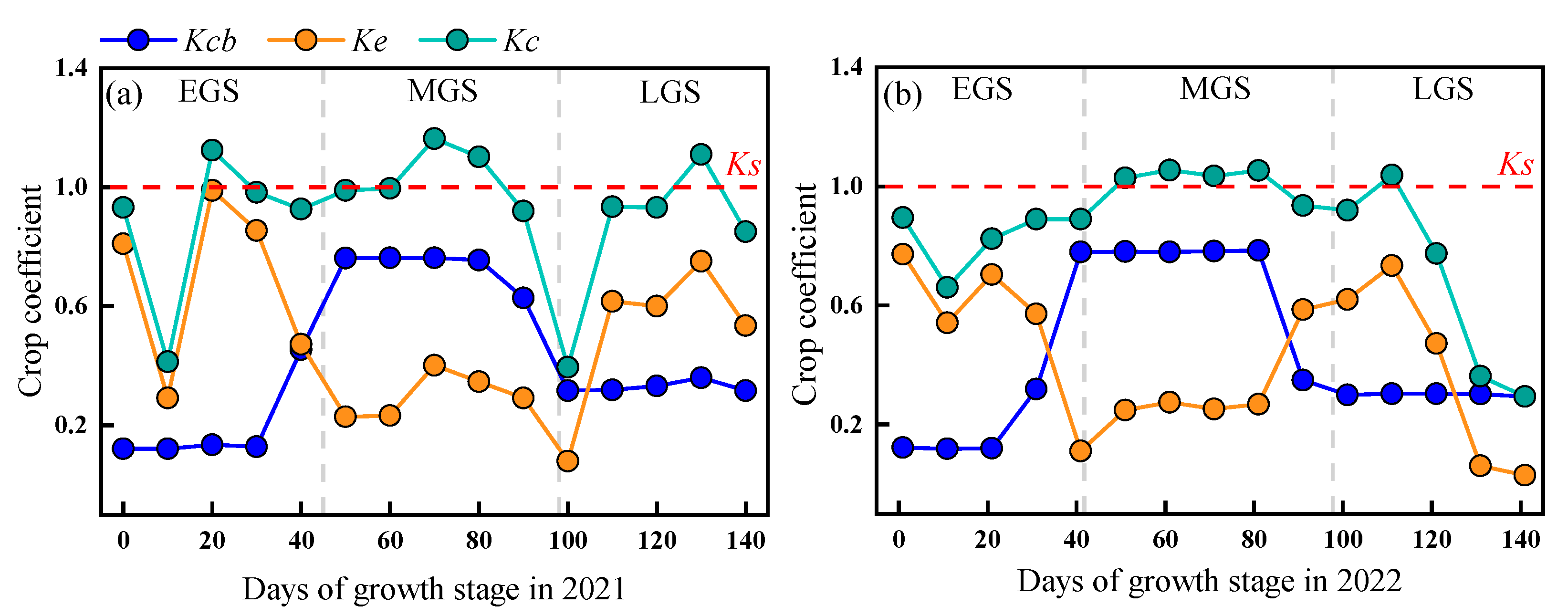
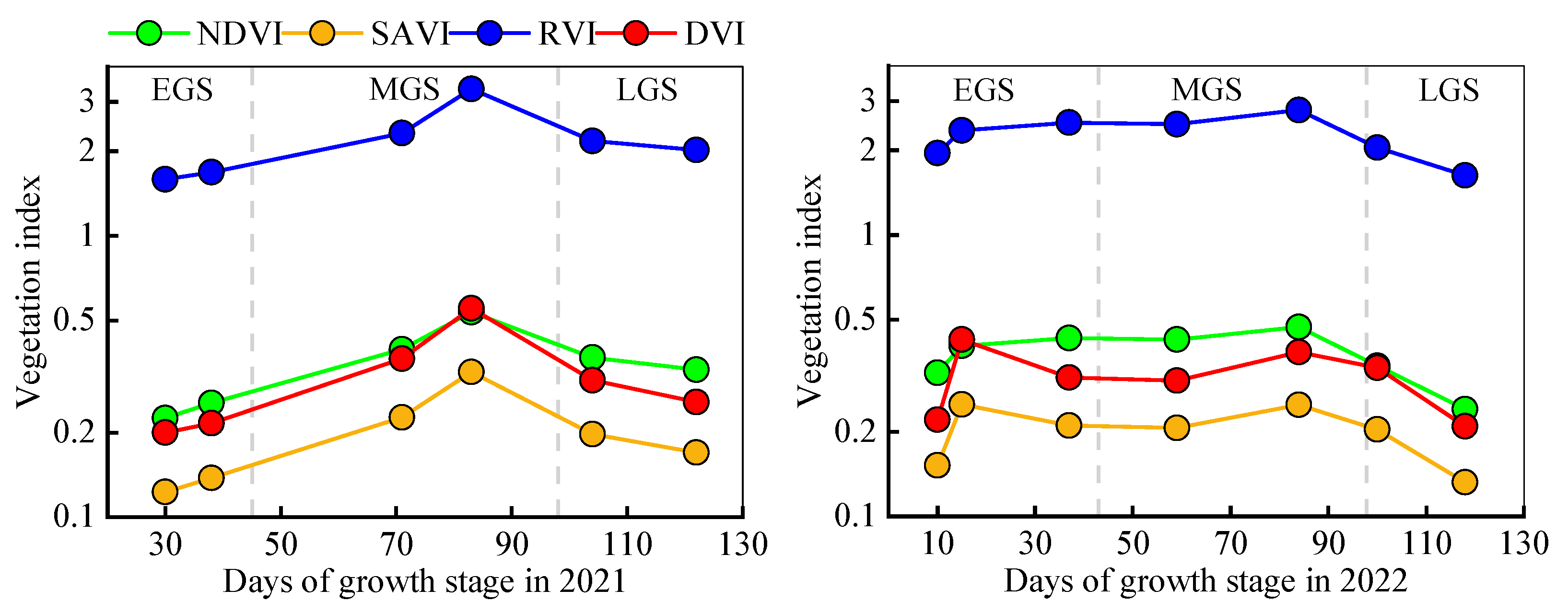
3.1. Grape Crop Coefficients and Vegetation Indices

The variation curves of the basal crop coefficient K_cb, soil evaporation coefficient K_e, water stress coefficient K_s, and crop coefficient K_c during the whole grape growth stage in 2021 and 2022 are shown in Figure 3. As illustrated, both years exhibited a similar trend in which the basal crop coefficient K_cb first increased and then decreased over the course of the growth stage. In 2021, K_cb was approximately 0.13 during the early growth stage, increased to about 0.76 in the mid-growth stage, and then decreased to around 0.33 in the late growth stage. A similar pattern was observed in 2022, with K_cb starting at about 0.12 in the early growth stage, reaching approximately 0.78 in the mid-growth stage, and then decreasing to around 0.30 in the late growth stage. The soil evaporation coefficient K_e exhibited a high value during the early growth stage, with measurements of approximately 0.71 in 2021 and 0.69 in 2022. As the vine canopy developed and coverage increased, K_e gradually decreased. In the mid-growth stage, K_e dropped to about 0.32 in 2021 and 0.23 in 2022. In the late growth stage, K_e values were approximately 0.49 in 2021 and 0.45 in 2022. Throughout the whole growth stage, no water stress was observed, which resulted in a constant water stress coefficient Ks of 1 in both years. As a result, the crop coefficient K_c was the sum of K_cb and K_e.

The correlation between vegetation indices and the basal crop coefficient (K_cb) of grapes was analyzed using Pearson correlation analysis, as shown in Figure 4. Excluding the VARI and GNDVI indices, the remaining six vegetation indices (NDVI, SAVI, RVI, EVI, ARVI, and DVI) showed strong correlations with the grape basal crop coefficient (K_cb), with correlation coefficients ranging from 0.648 to 0.742. Furthermore, these six indices exhibited high collinearity among themselves, with correlation coefficients between 0.830 and 0.987. Based on these findings, four vegetation indices (NDVI, SAVI, RVI, and DVI) with the highest correlations were selected for model development to link the vegetation indices to the grape basal crop coefficient K_cb. The variation curves of these four vegetation indices over the growing stage for both 2021 and 2022 are presented in Figure 5. As shown in Figure 5, the vegetation indices in both years initially increased slowly, followed by a gradual decrease, reflecting the typical growth and development pattern of the grapevines. As the vines began to bud, and new shoots emerged with leaves unfolding, the values of the vegetation indices increased. During the flowering and fruiting stages, the indices reached a saturation point. Finally, as the fruits ripened and the leaves began to yellow and fall, the values of the vegetation indices decreased [39].

3.2. Relationship Model Between Grape Basal Crop Coefficient with Vegetation Indices

In this study, four vegetation indices (NDVI, SAVI, RVI, DVI) were selected to establish univariate linear regression models, polynomial regression models, and multiple linear regression models to relate the vegetation indices to the grape basal crop coefficient (K_cb). The whole growth period was divided into two stages: the early growth stage and the late growth stage. The early growth stage encompassed the germination and flowering phases (prior to fruit development), while the late growth stage corresponded to the fruit expansion and coloring maturity phases. Relationship models between the selected vegetation indices and the grape basal crop coefficient (K_cb) were developed separately for each of these two stages.

The univariate linear regression relationships between grape vegetation indices with basal crop coefficient K_cb in the early and late growth stages of 2021 and 2022 are shown in

Table 3. The univariate linear regression relationships between grape vegetation indices with basal crop coefficient K_cb in the early and late growth stage in 2021 and 2022 (n = 15 in both stages of 2021, n = 11 in the early stage and n = 13 in the late stage of 2022).

Growth Stage	X	2021			2022
		Expression	R2	P	Expression	R2	P
Early growth stage	NDVI	y = 3.12x − 0.58	0.82	<0.001	y = 0.88x − 0.03	0.82	<0.001
	SAVI	y = 4.58x − 0.41	0.75	<0.01	y = 1.49x + 0.02	0.82	<0.001
	RVI	y = 0.70x − 0.98	0.80	<0.001	y = 0.15x − 0.03	0.74	<0.01
	DVI	y = 2.42x − 0.30	0.65	<0.01	y = 0.82x + 0.06	0.75	<0.01
Late growth stage	NDVI	y = 2.52x − 0.59	0.71	<0.01	y = 1.06x − 0.03	0.73	<0.01
	SAVI	y = 3.38x − 0.34	0.74	<0.01	y = 1.12x + 0.15	0.76	<0.01
	RVI	y = 0.40x − 0.55	0.75	<0.01	y = 0.12x + 0.09	0.80	<0.001
	DVI	y = 1.82x − 0.23	0.75	<0.01	y = 0.46x + 0.24	0.75	<0.01

. As shown in Table 3, the vegetation indices in both years demonstrated a satisfactory correlation with the grape basal crop coefficient (K_cb), with R² values exceeding 0.65 in 2021 and 0.73 in 2022.

The univariate linear regression models of the four vegetation indices with the grape basal crop coefficient K_cb for the whole growth stage in 2021 and 2022 are shown in Figure 6. As can be seen from Figure 6, the exponential fitting of the vegetation indices in 2021 yielded relatively stronger results. The coefficient of determination (R²) for the relationship between K_cb and the vegetation indices in 2021 was as follows: NDVI (R² = 0.67), SAVI (R² = 0.68), RVI (R² = 0.65), and DVI (R² = 0.66), with R² values generally above 0.65. In contrast, the coefficient of determination in 2022 was higher overall: NDVI (R² = 0.83), SAVI (R² = 0.67), RVI (R² = 0.75), and DVI (R² = 0.52). Apart from the DVI model, which has a relatively low fitting accuracy, the other models have good fitting accuracies, indicating that using vegetation indices to invert the grape basal crop coefficient K_cb was feasible. Since there were two stages of K_cb rising first and then decreasing in the process of grape growth, the same K_cb value could correspond to multiple vegetation index values. This phenomenon was more likely to occur in the middle of growth when the K_cb value was larger.

The polynomial regression relationships between grape vegetation indices with basal crop coefficient K_cb in the early and late growth stages of 2021 and 2022 are shown in

Table 4. The polynomial regression relationships between grape vegetation indices with basal crop coefficient K_cb in the early and late growth stage in 2021 and 2022 (n = 15 in both stages of 2021, n = 11 in the early stage and n = 13 in the late stage of 2022).

Growth Stage	X	2021			2022
		Expression	R2	P	Expression	R2	P
Early growth stage	NDVI	y = −3.74x2 + 5.48x − 0.93	0.83	<0.001	y = 4.21x2 − 1.53x + 0.28	0.89	<0.001
	SAVI	y = 38.98x2 − 8.64x + 0.58	0.75	<0.01	y = −2.69x2 + 2.33x − 0.04	0.83	<0.001
	RVI	y = 0.31x2 − 0.46x + 0.06	0.83	<0.001	y = 0.18x2 − 0.47x + 0.44	0.87	<0.001
	DVI	y = 3.41x2 + 0.61x − 0.1	0.68	<0.01	y = −2.12x2 + 1.93x − 0.07	0.82	<0.001
Late growth stage	NDVI	y = 9.36x2 − 5.52x + 1.04	0.77	<0.01	y = 1.3x2 − 0.12x + 0.21	0.77	<0.01
	SAVI	y = 12.51x2 − 2.86x + 0.37	0.77	<0.01	y = 0.46x2 + 0.78x + 0.2	0.76	<0.01
	RVI	y = 0.11x2 − 0.18x + 0.19	0.76	<0.01	y = 0.001x2 + 0.12x + 0.08	0.80	<0.001
	DVI	y = 3.06x2 − 0.69x + 0.22	0.76	<0.01	y = 0.02x2 + 0.42x + 0.25	0.75	<0.01

. As can be seen from Table 4, the R² values of vegetation indices and grape basal crop coefficient K_cb in the early and late growth stages of 2021 were higher (R² > 0.68), and the fitting effects were better in 2022 (R² > 0.75).

The polynomial regression models of four vegetation indices with grape basal crop coefficient K_cb in the whole growth stage in 2021 and 2022 are shown in Figure 7. As can be seen from Figure 7, the exponential fitting effects of four vegetation indices in 2021 were still stabler, with R² values ranging from 0.67 to 0.69. In 2022, the R² values were in the range of 0.66~0.85, respectively. Consistent with the univariate linear regression models during the same period, the NDVI model has the best fitting accuracy, while the DVI model showed the lowest accuracy. The data distribution in the figure was relatively balanced, indicating a good experimental period.

The independent variables selected in this study of the multiple linear regression models were x₁-NDVI, x₂-SAVI, x₃-RVI and x₄-DVI. The dependent variable was grape basal crop coefficient y-K_cb. The multiple linear regression models for the four vegetation indices with the grape basal crop coefficient K_cb in the early, late, and whole growth stages in 2021 and 2022 are shown in

Table 5. The multiple linear regression models of four vegetation indices with basic crop coefficient K_cb in different growth stages in 2021 and 2022 Table 5.

Growth Stage	2021				2022
	Model	R2	P	n	Model	R2	P	n
Early growth stage	y = 0.23 + 3.70x1 + 24.60x2 − 1.31x3 − 9.7x4	0.86	<0.001	15	y = 0.04 − 185.84x1 + 1185.92x2 + 0.42x3 − 545.67x4	0.96	<0.001	11
Late growth stage	y = −0.5 − 20.40x1 + 75.27x2 + 1.21x3 − 29.78x4	0.78	<0.01	15	y = −0.07 + 4.52x1 − 12.22x2 + 0.01x3 + 3.73x4	0.89	<0.001	13
Whole growth stage	y = −0.20 − 6.08x1 + 33.57x2 − 0.10x3 − 11.57x4	0.71	<0.01	30	y = −0.03 + 2.64x1 − 6.28x2 − 0.04x3 + 2.24x4	0.84	<0.001	24

. As shown in Table 5, the fitting accuracies of the K_cb-VIs multiple linear regression models in the early and late growth stages in 2021 were, respectively, 0.86 and 0.78, and the accuracy of the K_cb-VIs model in the whole growth stage was a little lower than the former two (R² = 0.71). All three have the highest model fitting accuracy during the same period. In 2022, the multiple linear regression model had a fitting accuracy of 0.96 in the early growth stage and 0.89 in the late growth stage, both higher than the fitting accuracy of the K_cb-VI_s model in the whole growth stage (R² = 0.84).

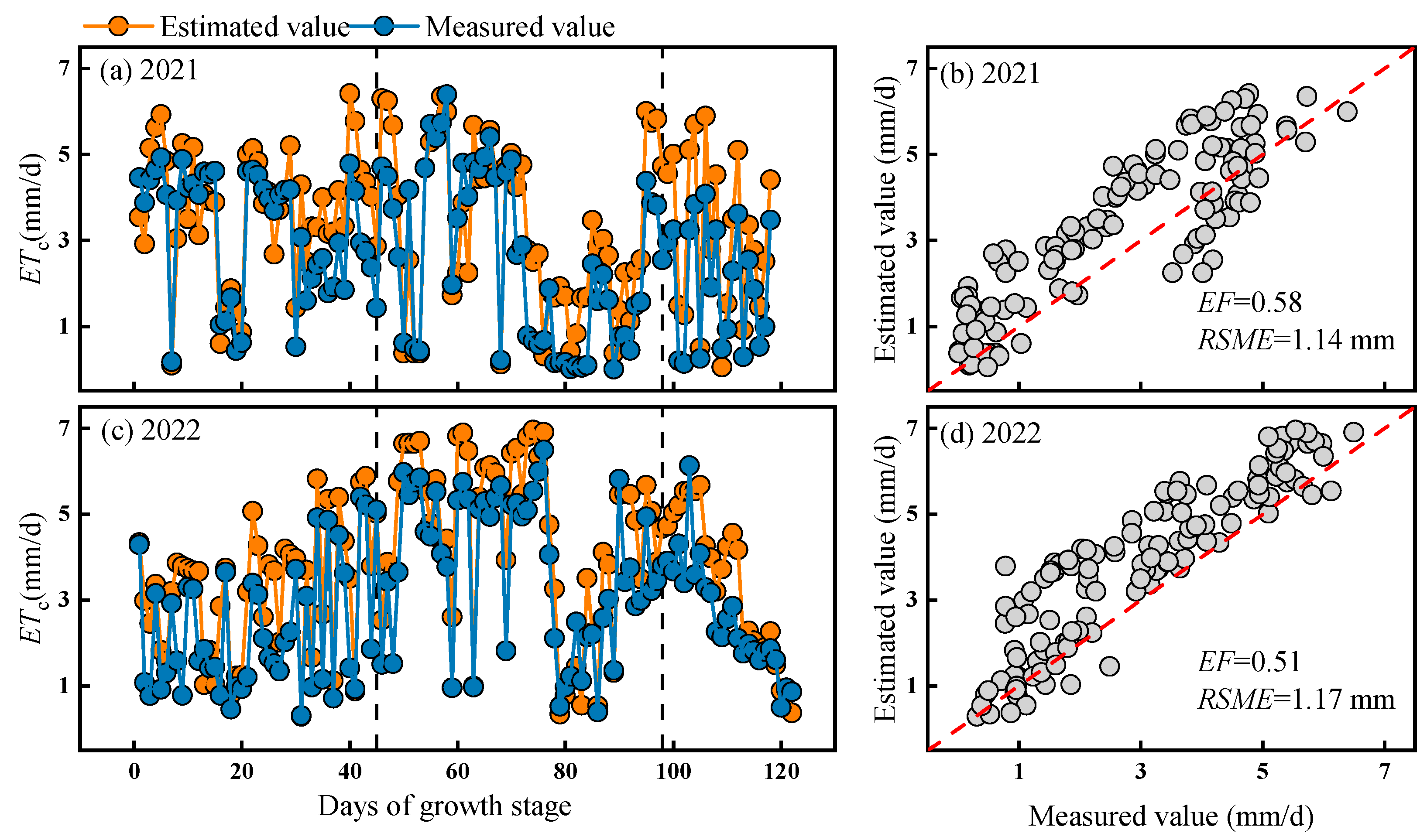
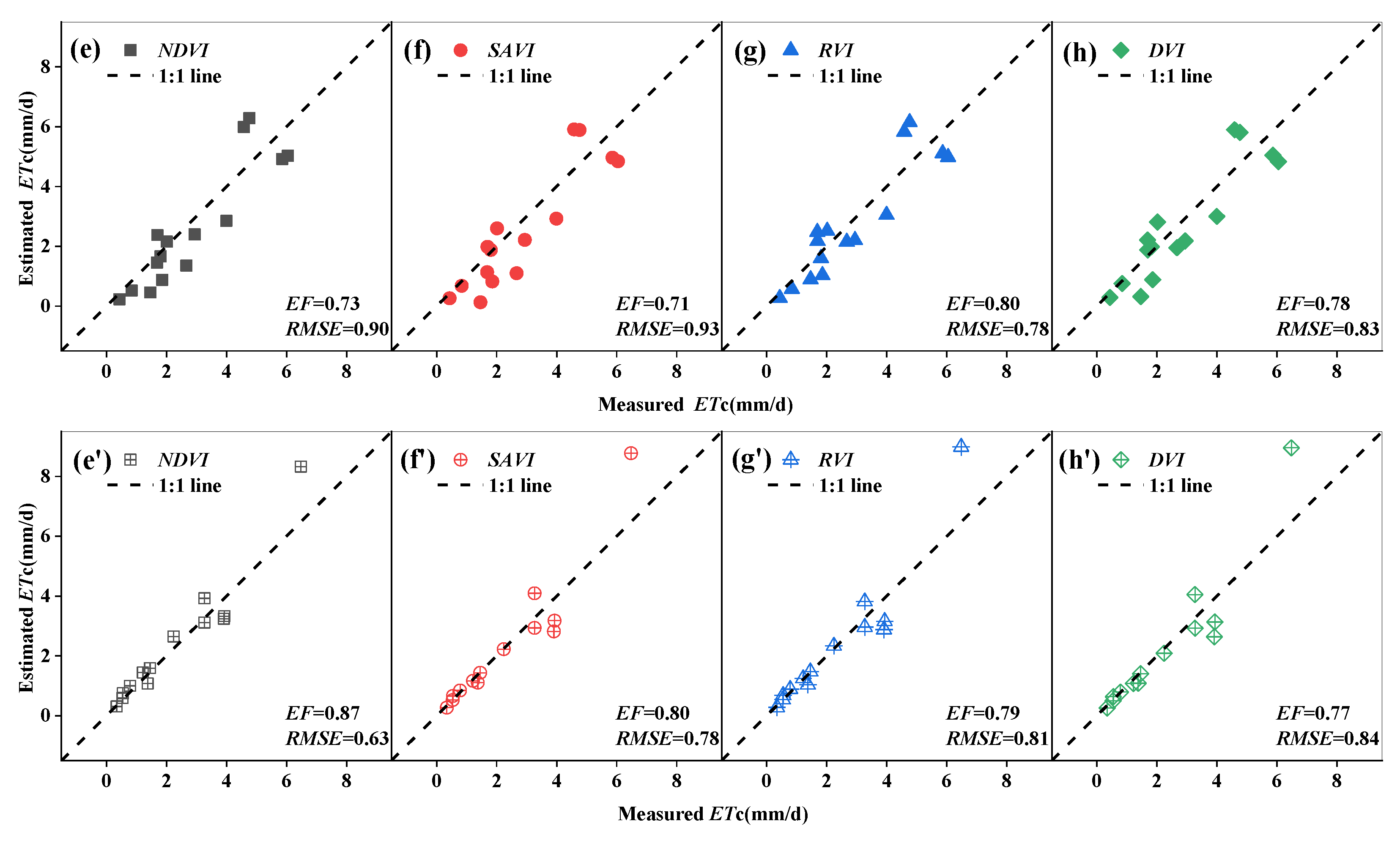
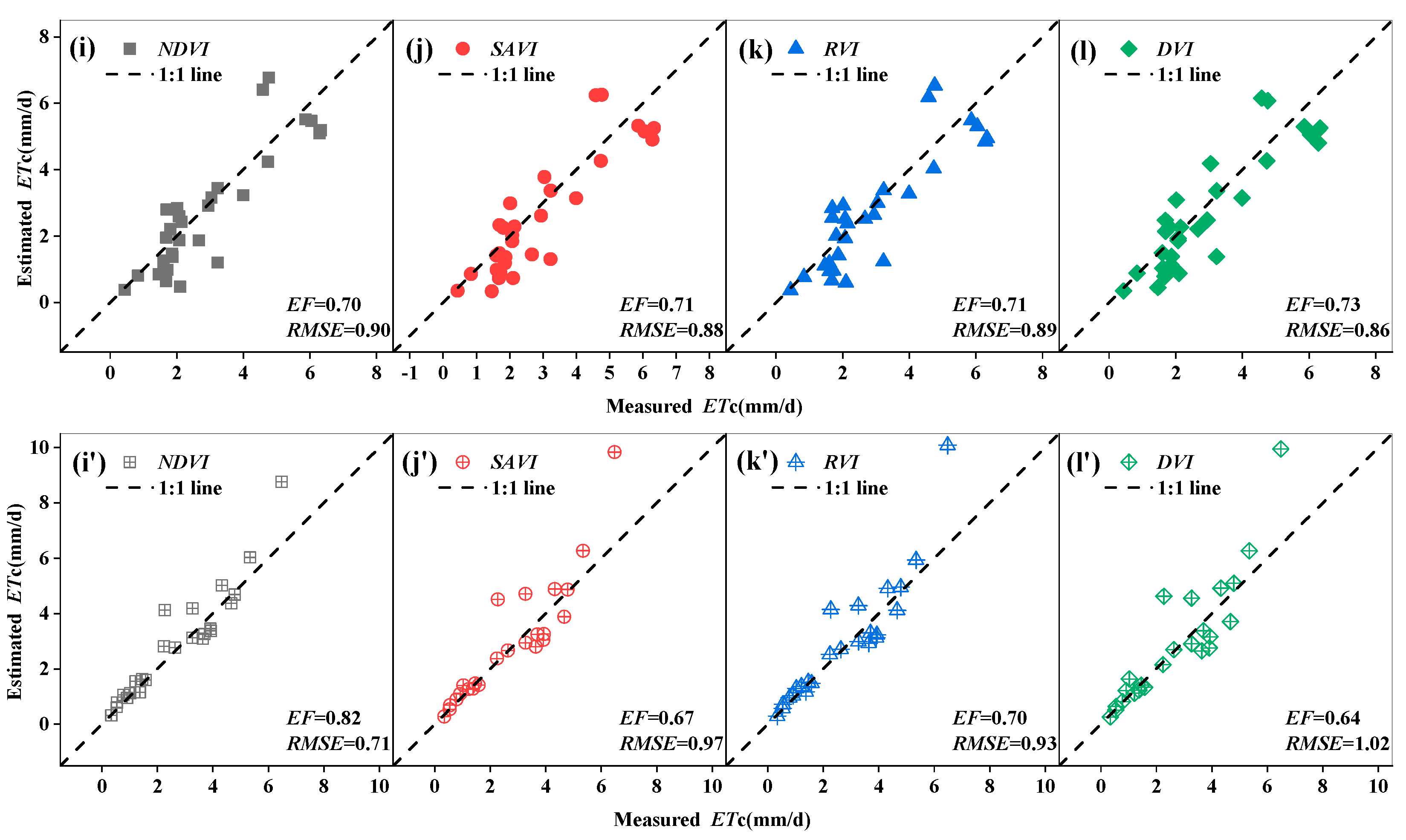
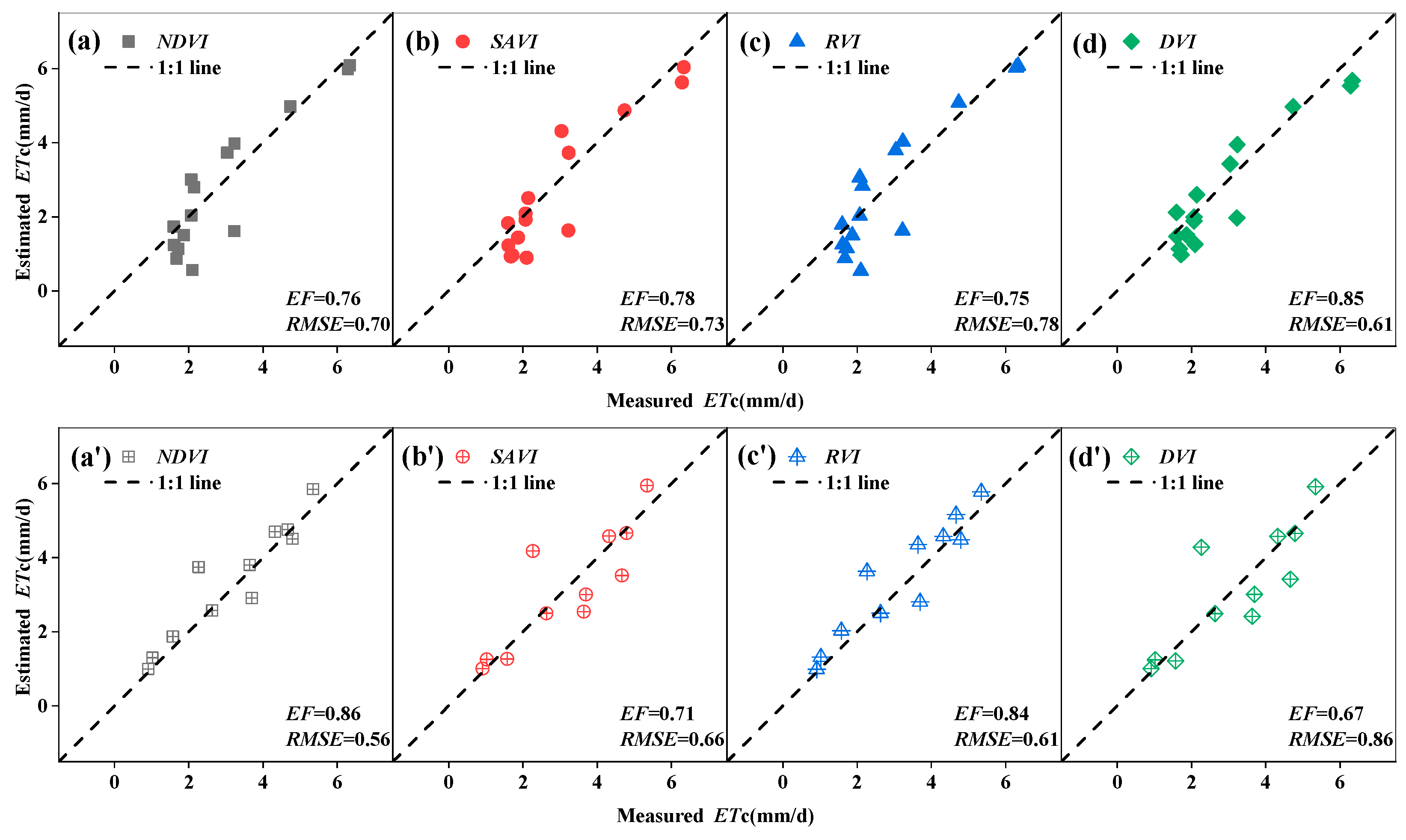
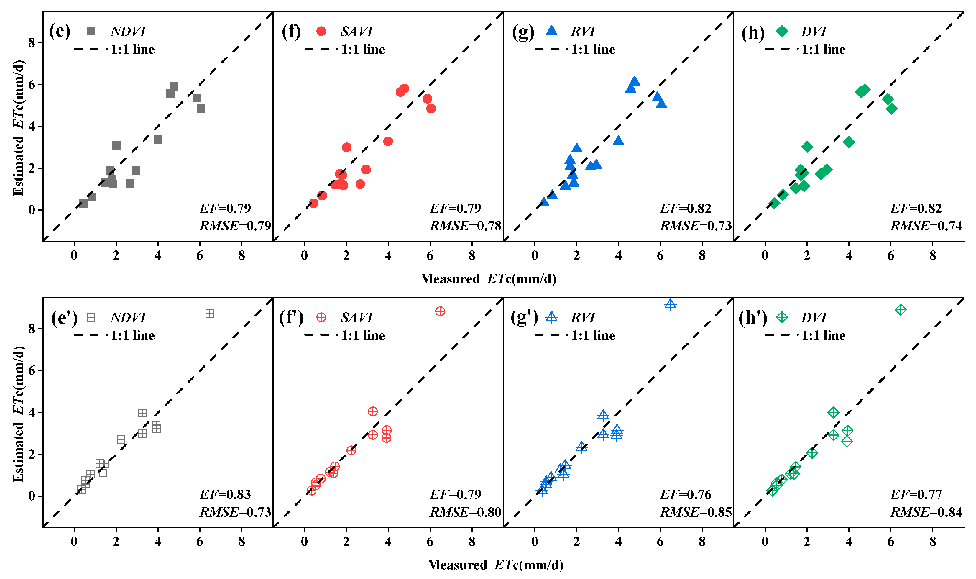
3.3. Verification of Evapotranspiration Model Estimation Accuracy

The daily grape evapotranspiration monitored automatically by the Bowen ratio system during the growing stage and its comparison with the evapotranspiration estimated by the FAO-56 dual crop coefficient method are shown in Figure 8. As can be seen from Figure 8, throughout the whole growing stage, the grape evapotranspiration exhibited an initial increase followed by a subsequent decrease. The fluctuations were relatively minor in the early and late growth stages, and the variation amplitude increased in the middle growth stage. The peak occurred in June, characterized by relatively low precipitation, abundant sunlight, and higher temperatures, coinciding with the period of most vigorous grape growth and the fruit enlargement stage. Conversely, the trough occurred in July, when rainfall was most concentrated. The variation range of the grape evapotranspiration in 2021 was 0.1 to 6.39 mm·d⁻¹ and in 2022 it was 0.31 to 6.50 mm·d⁻¹. From Figure 8, it can be seen that the grape evapotranspiration estimated by the FAO-56 recommended dual crop coefficient method was compared with the actual measurement value of the Bowen ratio system, and the accuracies were generally satisfactory (2021: n = 118, EF = 0.58; 2022: n = 122, EF = 0.51). The estimation values of the dual crop coefficient method are generally overestimated. This overestimation can be attributed to the crop coefficient being influenced by various factors, including climatic conditions, soil properties, crop cultivation management practices, and crop growth conditions, which collectively impose certain limitations on its estimation accuracies [40].

Using the univariate linear expressions of different vegetation indices with the grape basal crop coefficient K_cb obtained from Table 3 and Figure 6, K_cb was inverted to calculate the grape evapotranspiration in different growth stages for two years. These values were then compared with the values of grape evapotranspiration measured by the Bowen ratio system. The results are shown in Figure 9, Figure 10 and Figure 11.

As can be seen from Figure 9, in terms of the early growth stage, the vegetation indices with grape basal crop coefficient K_cb under the univariate linear modeling were used to estimate the grape evapotranspiration in 2021. The scatter points of NDVI, SAVI, RVI, and DVI were basically symmetrical and concentrated near the 1:1 line, with the estimation accuracies exceeding 0.71. In 2022, the model verification effects of NDVI and RVI reached 0.80, while the model verification effects for SAVI and DVI fell between 0.68 and 0.72.

For the late growth stage in 2021, as can be seen from Figure 10, the exponential model verification effects (EF = 0.71~0.80) were relatively stable, with the measured values being slightly higher than the predicted values. In 2022, the verification effects of the four vegetation indices, as determined by the exponential models (EF = 0.77–0.87), were improved, with the predicted values closely matching the measured values. However, when evapotranspiration was relatively high, the models tended to overestimate the actual values.

In the whole growth stage in 2021, as it can be seen from Figure 11, the differences in evapotranspiration by the four vegetation indices were not significant, and the RMSE values were consistently around 0.88 mm/d. In 2022, the verification accuracy of the four vegetation indices ranged between 0.64 and 0.82, with the NDVI model significantly outperforming the other three vegetation indices.

By comprehensively comparing the three growth stages in 2021 and 2022, the estimation accuracies of the grape basal crop coefficient K_cb based on vegetation indices through the univariate linear regression models were consistently above 0.64, indicating that using the univariate linear regression models to estimate evapotranspiration was feasible.

Using the polynomial regression relationships between different vegetation indices with the grape basal crop coefficient K_cb established in Table 4 and Figure 7, the grape evapotranspiration for the early, late, and whole growth stages in 2021 and 2022 was calculated. These estimates were then compared to the evapotranspiration values measured by the Bowen ratio system. The results are shown in Figure 12, Figure 13 and Figure 14.

As can be seen from Figure 12, in the early growth stage of 2021, compared with the univariate linear regression models, the polynomial regression model for DVI increased the estimation accuracy to 0.85. The improvements for the other three vegetation indices were relatively modest. In the early growth stage in 2022, compared with the univariate linear regression models, the estimation accuracy of the NDVI polynomial regression model was improved to 0.86. However, RVI was only slightly improved, while SAVI and DVI did not improve.

As can be seen from Figure 13, in the late growth stages in 2021 and 2022, the verification accuracies of the polynomial regression models for the four vegetation indices were above 0.76. When the evapotranspiration was high, the verification accuracies of the polynomial regression models decreased.

As can be seen from Figure 14, in 2021, in the whole growth stage, the verification accuracies of the four vegetation indices varied, but the differences were not significant. In 2022, in the whole growth stage, the NDVI and the RVI models had better verification results than the SAVI and the DVI models.

A comprehensive comparison of the scatter plots for the four vegetation indices during the three growth stages in both 2021 and 2022 revealed that the data points were symmetrically distributed and concentrated near the 1:1 line, indicating good verification results of the polynomial regression mode.

Following the development of the multiple linear regression models, as presented in Table 5, the grape evapotranspiration values for the early, late, and whole growth stages in 2021 and 2022 were calculated. These values were then compared to the measured evapotranspiration values from the Bowen ratio system, as shown in

Table 6. Verification of the estimation accuracies of the multiple linear regression models in the early, late, and whole growth stages.

Growth Stage	The Multiple Linear Regression Models
	2021		2022
	EF	RMSE/mm	EF	RMSE/mm
Early growth stage	0.81	0.69	0.77	0.69
Late growth stage	0.80	0.82	0.73	0.90
Whole growth stage	0.74	0.86	0.81	0.73

.

As can be seen from Table 6, in 2021, the estimation accuracies (EF = 0.81, 0.80) for the early and late growth stages were higher than the estimation accuracy (EF = 0.74) for the whole growth stage. In contrast, the estimation accuracy (EF = 0.81) for the whole growth stage was higher than the estimation accuracy (EF = 0.77) for the early growth stage and the estimation accuracy (EF = 0.73) for the late growth stage in 2022.

In summary, the multiple linear regression models demonstrated good estimation accuracies over the two years, outperforming most of the models during the same period.

4. Discussion

4.1. Data Analysis Required for the Model

The first part of this study primarily examines the temporal variations in grape crop coefficients and vegetation indices across the growth stages. The basal crop coefficient K_cb exhibited a characteristic parabolic trajectory, aligning with canonical grape developmental patterns. This variation primarily stems from dynamic canopy coverage changes. The FAO-56 guideline specifies K_cb values of 0.15, 0.80, and 0.40 for early, mid-, and late-season stages, respectively. Our observed values were systematically lower, attributable to variations in regional climate, cultivar-specific characteristics, and agricultural management practices [40]. Many scholars have improved the accuracy of evapotranspiration estimation by modifying the crop coefficient [41]. During vine development, the canopy coverage gradually increased, so crop transpiration was strengthened, and more soil moisture depletion occurred, leading to a progressive decline in K_e. In the late growth stage, as pruning activities and natural senescence of foliage for grape production gradually aged and faded, soil evaporation also increased gradually. Among them, the reason for the significant K_e variability in the early growth stage in 2021 was the soil moisture fluctuations caused by rainfall and irrigation. In the past two years, K_c gradually increased in the early growth stage, maintained a relatively stable and large value in the middle growth stage, and gradually decreased in the late growth stage. This pattern of change was consistent with that described in FAO-56. In 2022, K_c decreased rapidly in the late growth stage, mainly due to the rapid shift in soil evaporation coefficient in the late stage. The value of K_cb in the early and late stages of growth was small, so the changing trend of K_c was almost the same as that of K_e. The value of K_e was small in the middle growth stage; hence, the influence of K_cb on the K_c value was larger.

The changes in vegetation indices exhibited a strong correlation with the grape canopy coverage. From the early to the middle stage of growth, as the grape canopy cover increased, the vegetation indices also increased. From the middle to the late stage of growth, as the grape leaves gradually withered, the canopy cover decreased, and the vegetation indices also decreased. The values of vegetation indices are slightly lower than those in other studies [26,42]. We speculate that the differences may be due to the distinct grapevine varieties and the common practice of pruning branches and leaves to ensure better fruit growth in the local area. Additionally, the flight altitude of the UAV also has a certain impact on the acquisition of vegetation indices, and it should be adjusted according to the appropriate spatial resolution. Starting from the middle and late growth stage in 2021, RVI exhibited a pronounced downward trend. This was because RVI was sensitive to the change in crop coverage and particularly suited for monitoring the dynamic change of the canopy of plants with high coverage [43]. In 2022, the vegetation indices were higher in the early growth stage and reduced during mid-late phenological phases than in 2021. This was due to the influence of meteorological factors, which resulted in accelerated grape growth compared to 2021. There was no significant difference in the overall growth situation. DVI had a marked upward trajectory in the early growth stage, which was very sensitive to the change of soil background and influenced by inter-row cultivation practices.

4.2. Factors Affecting the Fitting Accuracy of the Model Between Grape Basal Crop Coefficient with Vegetation Indices

Over the course of two years, the models relating vegetation indices to the grape basal crop coefficient (K_cb), established at various growth stages using different methods, consistently yielded good results. This can be attributed to the ability of vegetation indices to reflect both vegetation coverage and growth activity, thereby quantifying the growth status of plants under specific conditions. The basal crop coefficient, which describes crop transpiration while excluding soil evaporation, was closely linked to crop growth. The changing patterns of vegetation indices were found to align closely with those of the grape basal crop coefficient (K_cb), demonstrating a strong correlation between the two [44].

4.2.1. The Growth Stage

Under the same modeling method, most vegetation indices followed the pattern that the model fitting accuracy was higher in the early growth stage than in the late growth stage. This was mainly because the vegetation indices were more sensitive to the grape basal crop coefficient K_cb when they were not saturated in the early growth stage. By the late growth stage, the vegetation indices reached a saturated state, and their sensitivity to the grape basal crop coefficient K_cb decreased. In 2021, except for DVI, the R² values for the other three vegetation indices in the early growth stage and the coefficient of grape basal crop K_cb were all higher than those in the late growth stage through the univariate linear regression modeling. The reason for this was that precipitation in the late growth stage, which primarily occurred in July and August, led to frequent rainfall and increased weed proliferation. If the weeding was delayed or the weed background was not properly removed in the late stage, it would affect the reflectivity of the extracted grape canopy and thus affect the calculation of vegetation indices. A similar situation was observed in the RVI model for 2022. Apart from the univariate linear regression models, the polynomial regression models and the multiple linear regression models also mostly followed the pattern of higher fitting accuracy in the early growth stage than in the late growth stage in both 2021 and 2022.

The differences in model accuracy between growth stages were likely due to the distinct growth conditions at each stage, which could lead to lower model fitting accuracy when the same relationship equation was applied across the whole growth period. In cases where the growth period was prolonged, it may be necessary to use multiple segmental relationships to more accurately express the variation trend of the grape basal crop coefficient (K_cb) throughout the whole growth stage. The results over the two years indicated that modeling by different growth stages yielded better-fitting results.

4.2.2. Type of Vegetation Index

Vegetation indices are simple, effective, and empirical measurement tools that reflect the condition of surface vegetation. They are widely used in global and regional land cover, vegetation classification, environmental change, primary productivity analysis, crop and forage yield estimation, drought monitoring, and other aspects [45,46,47,48,49].

The type of vegetation index was one of the most subjective factors affecting the model fitting accuracy. Different vegetation indices can yield different model fitting accuracies when the same modeling method was used in the same growth stage.

For example, when modeling using the univariate linear regression method, NDVI and RVI both have high and stable correlations with K_cb in different growth stages in two years. This was because NDVI and RVI could fully describe the difference in reflectance of vegetation in the near-infrared band and red band and also enhance the radiation difference between vegetation and soil background. They were the main means of estimating vegetation growth and abundance. The two bands had strong sensitivity to canopy transpiration, so they could well reflect crop transpiration capacity in different stages [43]. When using polynomial regression, the R² values of NDVI and RVI in the early growth stage were significantly higher than that in the late growth stage in 2021, and the R² value of DVI in the late growth stage was significantly higher than that in the early growth stage. The main reason for this difference was that NDVI and RVI were more sensitive to vegetation coverage and vegetation growth status, with higher sensitivity in the early growth stage when vegetation was not yet saturated. In contrast, DVI focused more on changes in soil background and was less affected by weeding activities in the late growth stage. In comparison, when using the same modeling method at each stage, the SAVI models had a moderate fitting accuracy and performed more stably. Taking all factors into consideration, NDVI was more suitable for fitting in the early growth stage and the whole growth period, while RVI was more appropriate for fitting in the late growth stage.

4.2.3. Modeling Method

The three modeling methods selected in this study are commonly used, with simple calculations and low data volume requirements, and have relatively few limitations in various aspects.

A comparison of the fitting accuracies between the univariate linear regression models and polynomial regression models revealed that the R² values for vegetation indices with grape basal crop coefficient (K_cb) established through the polynomial regression models were generally higher than those from the univariate linear regression models across all growth stages. However, the degree of improvement was not substantial. This was primarily because the K_cb models for monomial vegetation indices inversion of grape crop coefficients exhibited high fitting accuracies. Nevertheless, these two models considered the influence of single variable factors on dependent variables and could not fully consider the influence degree of various factors on crop coefficient. Therefore, there was no significant difference in the improvement effect, which was consistent with the research results of Han Wenting [24].

When comparing the multiple linear regression models, it was found that, with the exception of the NDVI polynomial regression model for the whole growth stage (R² = 0.85), the accuracies of the multiple linear regression models were higher than those of the univariate linear regression models and polynomial regression models at the same stage. This was due to the fact that the multiple linear regression models did not only consider the influence of one vegetation index on K_cb but also incorporated a variety of vegetation indices for a more comprehensive assessment. Furthermore, the correlation between independent variables and multiple dependent variables was improved [50].

4.3. Comparison of Evapotranspiration Models

The three types of evapotranspiration estimation models based on unmanned aerial vehicle (UAV) multispectral remote sensing have shown good verification results over the two years, with EF ranging from 0.64 to 0.87 and RMSE from 0.56 to 1.02 mm/d, both higher than the estimation accuracy of the FAO-56 recommended dual crop coefficient method (2021: EF = 0.58; 2022: EF = 0.51). This indicated that using the Bowen ratio system as a benchmark, inverting the grape basal crop coefficient based on UAV multispectral remote sensing to estimate grape evapotranspiration using the dual crop coefficient method was feasible. The study identified three important factors influencing the fitting accuracy of the K_cb-VI_s model: growth stage, type of vegetation index, and modeling method. The fitting accuracy, in turn, influenced the model’s estimation of evapotranspiration, specifically the model verification accuracy.

(1)

Growth Stage: When comparing the verification accuracy of the four vegetation indices under different modeling methods in the early, late, and whole growth stages, it was observed that for most models in 2021 and 2022, the verification accuracy in the early and late growth stages was higher than that in the whole growth stage. This was because the grape growth period was relatively long, making it necessary to estimate evapotranspiration separately for each growth stage to ensure accuracy. Using the same fitting formula for the whole growth period would lead to a decrease in accuracy due to the mismatch between flight frequency and grape growth rate. The difference in verification accuracy of grape evapotranspiration in the early and late growth stages was mainly due to external factors such as weed growth and internal factors such as whether the vegetation indices reached saturation in the late growth stage.

(2)

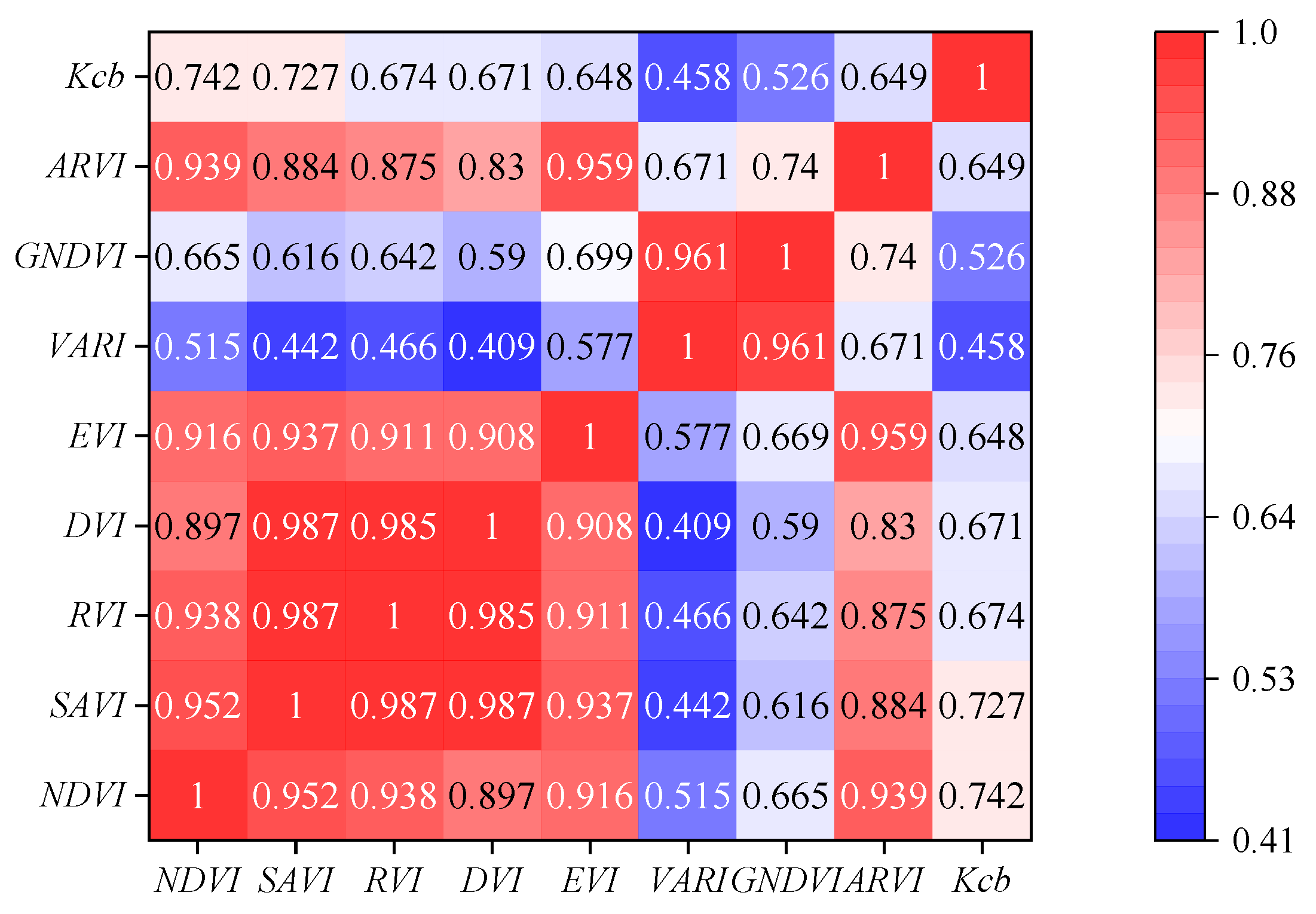
Types of Vegetation Index: The four vegetation indices led to differences in verification accuracy due to varying model fitting accuracies. When the fitting accuracy of a vegetation index was high, the model verification accuracy also tended to improve. Under both univariate linear regression and polynomial regression modeling, the highest accuracy for estimating evapotranspiration using NDVI was 0.87, with an RMSE of 0.63 mm/d. In contrast, the DVI model had the poorest validation results, with an accuracy of only 0.64 and an RMSE of 1.02 mm/d. The larger RMSE may be due to the fact that larger errors, when squared, increase the gap between the estimated and actual values.

(3)

Modeling Methods: The same vegetation index under the same growth stage may have different model verification accuracies due to different modeling methods. In 2021 and 2022, the verification accuracies of the polynomial regression models were slightly higher than that of the univariate linear regression models. This indicated that when the verification accuracies of the univariate linear regression models were high, the polynomial regression model may improve the verification accuracy because non-linear fitting had a certain impact on improving model verification accuracy. However, it cannot significantly enhance the accuracy, as both modeling methods only consider a single factor. In contrast, the multiple linear regression model had the highest validation accuracy, suggesting that considering multiple vegetation indices comprehensively can improve the model verification accuracy.

For example, in the early growth stage of 2021, compared to the univariate linear regression models, the estimation accuracy of the DVI polynomial regression model increased to 0.85, while the other three vegetation indices only showed slight improvements. In the early growth stage of 2022, compared to the univariate linear regression models, the estimation accuracy of the NDVI polynomial regression model increased to 0.86, with only a slight improvement for RVI and no improvement for SAVI and DVI. This indicated that using polynomials did not always enhance the verification results. This was mainly because, on one hand, the univariate linear regression model had already achieved high estimation accuracy. On the other hand, the polynomial regression models failed to effectively address the issue of decreasing estimation accuracy as evapotranspiration increased within the same growth stage, which even led to a tendency to further increase the error.

In 2021 and 2022, the verification accuracy of the multiple linear regression models did not show a significant improvement compared to the univariate linear regression and polynomial regression models in the early and late growth stages. This was mainly because the multiple linear regression models introduced multiple vegetation index feature parameters, increasing the model complexity [51]. Additionally, the four vegetation indices selected in this study either had limited applicability or strong collinearity among them, which affected the simulation. However, during the whole growth stage, the estimation accuracies of the multiple linear regression models were better than those of the univariate linear regression and polynomial regression models. This indicated that considering multiple influencing factors during this period better simulated the changes in the grape basal crop coefficient K_cb, thereby enabling more accurate estimations of grape evapotranspiration.

Based on the comparison of the verification accuracies of evapotranspiration models, it was recommended to use the NDVI polynomial regression models in the early growth stage for the best results; the RVI univariate linear regression models had the best accuracies in the late growth stage; and the multiple linear regression models were more stable for the whole growth stage.

4.4. Limitations and Future Research

Due to the significant impact of factors such as solar altitude angle and radiation intensity on the spectral characteristics of grape, unmanned aerial vehicle (UAV) multispectral remote sensing has higher requirements for favorable weather conditions and precise timing of the experiment on the trial day. Furthermore, the three types of UAV multispectral models require a large amount of experimental data to model the grape basal crop coefficient. Estimating evapotranspiration through the inversion of the basal crop coefficient is relatively complex, and the modeling accuracy can affect the estimation accuracy. However, the advantage is that the basal crop coefficient does not change significantly over short periods, making the dual crop coefficient method more suitable for estimating evapotranspiration over stages. Although it is feasible to estimate the grape basal crop coefficient using unmanned aerial vehicle (UAV) multispectral remote sensing to estimate evapotranspiration during the growth period, a limitation is that this method provides estimates on a daily scale. How to ensure high evapotranspiration estimation accuracy over the entire growth period with a limited number of flight trials remains to be studied. How to ensure high evapotranspiration estimation accuracy over the whole growth stage with a limited number of flight trials remains to be studied. Moreover, how to account for the differences in evapotranspiration caused by individual plant variations to expand the spatial scale has not yet been resolved. Additionally, this study only inverts the basal crop coefficient, lacking the means to correct the soil evaporation coefficient through UAV multispectral remote sensing to improve the dual crop coefficient method. Future research can enhance the accuracy of evapotranspiration estimation by incorporating the inversion of the soil evaporation coefficient.

5. Conclusions

This article used the actual evapotranspiration ET_c measured by the Bowen ratio system as the baseline, calculated the reference crop evapotranspiration ET_o based on the Penman formula, and obtained the grape crop coefficient K_c. The FAO-56 dual crop coefficient method was then employed to calculate the soil evaporation coefficient K_e and the water stress coefficient K_s, thereby deriving the basal crop coefficient K_cb. Simultaneously, UAV multispectral remote sensing images were used to obtain grape spectral data, extracted reflectance from multiple bands to calculate four vegetation indices, and established relationship models between the grape basal crop coefficient K_cb with vegetation indices using different methods. This study identified that the growth stage, type of vegetation index, and modeling method were three important factors affecting the fitting accuracies of the K_cb-VI_s models. In 2021 and 2022, most vegetation indices followed the pattern that the fitting accuracies were highest in the early growth stage, followed by the late growth stage, and then the whole growth stage, regardless of the modeling method used. In both years, for the early growth stage and the whole growth stage, the K_cb-VI_s models obtained using the univariate linear regression and the polynomial regression had good fitting accuracies for NDVI, while in the late growth stage, the models based on RVI had the best fitting effects. Different modeling methods have different fitting accuracies for the grape basal crop coefficient K_cb, with the multiple linear regression models having the best fitting effects, followed by the polynomial regression models, and then the univariate linear regression models.

Using the inverted K_cb values from the models to re-estimate the grape evapotranspiration with the dual crop coefficient method and comparing them with the measured values, it was found that the fitting accuracies of the K_cb-VI_s models affected the estimation accuracies of evapotranspiration. Over the two years, different inversion models showed good performance in estimating the evapotranspiration of grape, though the results varied. Based on the growth characteristics of grape, using UAV multispectral remote sensing to select appropriate vegetation indices and modeling methods for different growth stages to invert K_cb values can improve the estimation accuracies of evapotranspiration by more than 11% in 2021 and 13% in 2022 compared to the K_cb recommended values of FAO-56. A comparison of the verification accuracies of the evapotranspiration models led to the following recommendations: NDVI polynomial regression models should be used for the early growth stage to achieve optimal results; RVI univariate linear regression models are most accurate for the late growth stage; and multiple linear regression models provide more stable performance for the entire growth period.

References

1. Xu, C.-Y.; Singh, V.P. Evaluation of Three Complementary Relationship Evapotranspiration Models by Water Balance Approach to Estimate Actual Regional Evapotranspiration in Different Climatic Regions. J. Hydrol. 2005, 308, 105–121. [Google Scholar] [CrossRef]
2. Ferreira, M.I.; Silvestre, J.; Conceição, N.; Malheiro, A.C. Crop and Stress Coefficients in Rainfed and Deficit Irrigation Vineyards Using Sap Flow Techniques. Irrig. Sci. 2012, 30, 433–447. [Google Scholar] [CrossRef]
3. Cui, N.; He, Z.; Jiang, S.; Wang, M.; Yu, X.; Zhao, L.; Qiu, R.; Gong, D.; Wang, Y.; Feng, Y. Inter-Comparison of the Penman-Monteith Type Model in Modeling the Evapotranspiration and Its Components in an Orchard Plantation of Southwest China. Agric. Water Manag. 2023, 289, 108541. [Google Scholar] [CrossRef]
4. Li, X.H.; Liu, H.J.; Wang, Y.; Wang, L.G.; Pei, X.Y.; Wu, Y.B.; Zheng, G.Q. Chinese grape Market and Industry survey analysis report. Agric. Prod. Mark. 2021, 18, 49–51. [Google Scholar]
5. Wang, Q.L.; Zhao, Y.Y.; Guo, J.Q.; Wang, Y.W.; Zhang, X.Y.; Wang, X.P. Investigation on the introduction performance of eleven table grape varieties in Yan-gling, Shaanxi Province. Northwest Hortic. (Fruit Trees) 2021, 04, 46–49. [Google Scholar]
6. Yu, Z.; Hu, X.; Ran, H.; Wang, X.; Wang, W.; He, X. Estimation of Evapotranspiration in Vine-yards of Semi-Humid Areas Based on the Bowen Ratio-Energy Balance Method. Agric. Res. Arid. Areas 2020, 38, 9. [Google Scholar] [CrossRef]
7. Williams, D.G.; Cable, W.; Hultine, K.; Hoedjes, J.C.B.; Yepez, E.A.; Simonneaux, V.; Er-Raki, S.; Boulet, G.; De Bruin, H.A.R.; Chehbouni, A.; et al. Evapotranspiration Components Determined by Stable Isotope, Sap Flow and Eddy Covariance Techniques. Agric. For. Meteorol. 2004, 125, 241–258. [Google Scholar] [CrossRef]
8. A Review of the Bowen Ratio Surface Energy Balance Method for Quantifying Evapotranspiration and Other Energy Fluxes. Trans. ASABE 2014, 1657–1674. [CrossRef]
9. Ding, R.; Kang, S.; Li, F.; Zhang, Y.; Tong, L.; Sun, Q. Evaluating Eddy Covariance Method by Large-Scale Weighing Lysimeter in a Maize Field of Northwest China. Agric. Water Manag. 2010, 98, 87–95. [Google Scholar] [CrossRef]
10. Ai, P.; Ma, Y. Estimation of Evapotranspiration of a Jujube/Cotton Intercropping System in an Arid Area Based on the Dual Crop Coefficient Method. Agriculture 2020, 10, 65. [Google Scholar] [CrossRef]
11. Han, J.; Tian, L.; Cai, Z.; Ren, W.; Liu, W.; Li, J.; Tai, J. Season-Specific Evapotranspiration Partitioning Using Dual Water Isotopes in a Pinus Yunnanensis Ecosystem, Southwest China. J. Hydrol. 2022, 608, 127672. [Google Scholar] [CrossRef]
12. Foken, T.; Aubinet, M.; Leuning, R. The Eddy Covariance Method. In Eddy Covariance; Aubinet, M., Vesala, T., Papale, D., Eds.; Springer Netherlands: Dordrecht, The Netherlands, 2012; pp. 1–19. ISBN 978-94-007-2350-4. [Google Scholar]
13. Paço, T.A.; Ferreira, M.I.; Rosa, R.D.; Paredes, P.; Rodrigues, G.C.; Conceição, N.; Pacheco, C.A.; Pereira, L.S. The Dual Crop Coefficient Approach Using a Density Factor to Simulate the Evapotranspiration of a Peach Orchard: SIMDualKc Model versus Eddy Covariance Measurements. Irrig. Sci. 2012, 30, 115–126. [Google Scholar] [CrossRef]
14. Phogat, V.; Šimůnek, J.; Skewes, M.A.; Cox, J.W.; McCarthy, M.G. Improving the Estimation of Evaporation by the FAO-56 Dual Crop Coefficient Approach under Subsurface Drip Irrigation. Agric. Water Manag. 2016, 178, 189–200. [Google Scholar] [CrossRef]
15. Flumignan, D.L.; De Faria, R.T.; Prete, C.E.C. Evapotranspiration Components and Dual Crop Coefficients of Coffee Trees during Crop Production. Agric. Water Manag. 2011, 98, 791–800. [Google Scholar] [CrossRef]
16. Santosh, D.T.; Tiwari, K.N. Estimation of Water Requirement of Banana Crop under Drip Irrigation with and without Plastic Mulch Using Dual Crop Coefficient Approach. IOP Conf. Ser. Earth Environ. Sci. 2019, 344, 012024. [Google Scholar] [CrossRef]
17. Glenn, E.P.; Neale, C.M.U.; Hunsaker, D.J.; Nagler, P.L. Vegetation Index-based Crop Coefficients to Estimate Evapotranspiration by Remote Sensing in Agricultural and Natural Ecosystems. Hydrol. Process. 2011, 25, 4050–4062. [Google Scholar] [CrossRef]
18. Hunsaker, D.J.; Pinter, P.J.; Barnes, E.M.; Kimball, B.A. Estimating Cotton Evapotranspiration Crop Coefficients with a Multispectral Vegetation Index. Irrig. Sci. 2003, 22, 95–104. [Google Scholar] [CrossRef]
19. Sankaran, S.; Khot, L.R.; Carter, A.H. Field-Based Crop Phenotyping: Multispectral Aerial Imaging for Evaluation of Winter Wheat Emergence and Spring Stand. Comput. Electron. Agric. 2015, 118, 372–379. [Google Scholar] [CrossRef]
20. Shi, Y.; Thomasson, J.A.; Murray, S.C.; Pugh, N.A.; Rooney, W.L.; Shafian, S.; Rajan, N.; Rouze, G.; Morgan, C.L.S.; Neely, H.L.; et al. Unmanned Aerial Vehicles for High-Throughput Phenotyping and Agronomic Research. PLoS ONE 2016, 11, e0159781. [Google Scholar] [CrossRef]
21. Han, W.T.; Zhang, L.Y.; Niu, Y.X.; Shi, X. Research progress of UAV remote sensing technology in precision irrigation. Trans. Chin. Soc. Agric. Mach. 2020, 51, 1–14. [Google Scholar]
22. Marcial-Pablo, M.D.J.; Ontiveros-Capurata, R.E.; Jiménez-Jiménez, S.I.; Ojeda-Bustamante, W. Maize Crop Coefficient Estimation Based on Spectral Vegetation Indices and Vegetation Cover Fraction Derived from UAV-Based Multispectral Images. Agronomy 2021, 11, 668. [Google Scholar] [CrossRef]
23. Zhang, Y.; Zhang, L.; Zhang, H.; Song, Z.; Lin, G.; Han, W. Study on Estimation Method of Corn Crop Coefficient Using UAV Remote Sensing in Conjunction with Ground Water Monitoring. Trans. Chin. Soc. Agric. Eng. 2019, 35, 7. [Google Scholar] [CrossRef]
24. Han, W.T.; Shao, G.M.; Ma, D.J.; Wang, Y.; Niu, Y.X. Uav multi-spectral Remote sensing method for estimation of maize crop coefficient in field. Trans. Chin. Soc. Agric. Mach. 2018, 49, 134–143. [Google Scholar] [CrossRef]
25. Shao, G.; Han, W.; Zhang, H.; Liu, S.; Wang, Y.; Zhang, L.; Cui, X. Mapping Maize Crop Coefficient Kc Using Random Forest Algorithm Based on Leaf Area Index and UAV-Based Multispectral Vegetation Indices. Agric. Water Manag. 2021, 252, 106906. [Google Scholar] [CrossRef]
26. Gautam, D.; Ostendorf, B.; Pagay, V. Estimation of Grapevine Crop Coefficient Using a Multispectral Camera on an Unmanned Aerial Vehicle. Remote Sens. 2021, 13, 2639. [Google Scholar] [CrossRef]
27. Wei, H.; Wang, J.; Li, M.; Wen, M.; Lu, Y. Assessing the Applicability of Mainstream Global Isoscapes for Predicting δ18O, δ2H, and d-Excess in Precipitation across China. Water 2023, 15, 3181. [Google Scholar] [CrossRef]
28. Dicken, U.; Cohen, S.; Tanny, J. Examination of the Bowen Ratio Energy Balance Technique for Evapotranspiration Estimates in Screenhouses. Biosyst. Eng. 2013, 114, 397–405. [Google Scholar] [CrossRef]
29. Allen, R.G.; Pereira, L.S.; Raes, D.; Smith, M. Crop Evapotraspiration—Guidelines for Computing Crop Water Requirements—FAO Irrigation& Drainage; FAO: Roma, Italy, 1998; p. 56. [Google Scholar]
30. Bannari, A.; Morin, D.; Bonn, F.; Huete, A.R. A Review of Vegetation Indices. Remote Sens. Rev. 1995, 13, 95–120. [Google Scholar] [CrossRef]
31. Huete, A.R. A Soil-Adjusted Vegetation Index (SAVI). Remote Sens. Environ. 1988, 25, 295–309. [Google Scholar] [CrossRef]
32. Priebe, S.; Huxley, P.; Knight, S.; Evans, S. Application and Results of the Manchester Short Assessment of Quality of Life (Mansa). Int. J. Soc. Psychiatry 1999, 45, 7–12. [Google Scholar] [CrossRef] [PubMed]
33. Richardson, A.J. Distinguishing Vegetation from Soil Background Information. Photogramm. Eng. Remote Sens. 1977, 43, 1541–1552. [Google Scholar]
34. Huete, A.; Didan, K.; Miura, T.; Rodriguez, E.P.; Gao, X.; Ferreira, L.G. Overview of the Radiometric and Biophysical Performance of the MODIS Vegetation Indices. Remote Sens. Environ. 2002, 83, 195–213. [Google Scholar] [CrossRef]
35. Schneider, P.; Roberts, D.A.; Kyriakidis, P.C. A VARI-Based Relative Greenness from MODIS Data for Computing the Fire Potential Index. Remote Sens. Environ. 2008, 112, 1151–1167. [Google Scholar] [CrossRef]
36. Wang, F.; Huang, J.; Tang, Y.; Wang, X. New Vegetation Index and Its Application in Estimating Leaf Area Index of Rice. Rice Sci. 2007, 14, 195–203. [Google Scholar] [CrossRef]
37. Kaufman, Y.J.; Tanre, D. Atmospherically Resistant Vegetation Index (ARVI) for EOS-MODIS. IEEE Trans. Geosci. Remote Sens. 1992, 30, 261–270. [Google Scholar] [CrossRef]
38. Zheng, W.S.; Zhang, G.Z.; Zhang, Z.X.; Zheng, L. Modeling and evaluation of maize water production function in semi-arid region of western Heilongjiang Province. J. Northeast. Agric. Univ. 2011, 42, 61–65. [Google Scholar]
39. Peng, X.; Chen, D.; Zhou, Z.; Zhang, Z.; Xu, C.; Zha, Q.; Wang, F.; Hu, X. Prediction of the Nitrogen, Phosphorus and Potassium Contents in Grape Leaves at Different Growth Stages Based on UAV Multispectral Remote Sensing. Remote Sens. 2022, 14, 2659. [Google Scholar] [CrossRef]
40. Zhao, P.; Kang, S.; Li, S.; Ding, R.; Tong, L.; Du, T. Seasonal Variations in Vineyard ET Partitioning and Dual Crop Coefficients Correlate with Canopy Development and Surface Soil Moisture. Agric. Water Manag. 2018, 197, 19–33. [Google Scholar] [CrossRef]
41. Ding, R.; Kang, S.; Zhang, Y.; Hao, X.; Tong, L.; Du, T. Partitioning Evapotranspiration into Soil Evaporation and Transpiration Using a Modified Dual Crop Coefficient Model in Irrigated Maize Field with Ground-Mulching. Agric. Water Manag. 2013, 127, 85–96. [Google Scholar] [CrossRef]
42. Xia, T.; Kustas, W.P.; Anderson, M.C.; Alfieri, J.G.; Gao, F.; McKee, L.; Prueger, J.H.; Geli, H.M.E.; Neale, C.M.U.; Sanchez, L.; et al. Mapping Evapotranspiration with High-Resolution Aircraft Imagery over Vineyards Using One- and Two-Source Modeling Schemes. Hydrol. Earth Syst. Sci. 2016, 20, 1523–1545. [Google Scholar] [CrossRef]
43. Li, H. Experiment and analysis of NDVI and RVI inversion results based on Landsat image. Geospat. Inf. 2021, 19, 75–77. [Google Scholar]
44. Shao, G.; Wang, Y.; Han, W. Estimation Method of Leaf Area Index of Summer Corn Based on UAV Multi-spectral Remote Sensing. Smart Agric. 2020, 2, 11. [Google Scholar] [CrossRef]
45. Jin, X.; Li, Z.; Feng, H.; Ren, Z.; Li, S. Deep Neural Network Algorithm for Estimating Maize Biomass Based on Simulated Sentinel 2A Vegetation Indices and Leaf Area Index. Crop J. 2020, 8, 87–97. [Google Scholar] [CrossRef]
46. Alam, M.S.; Lamb, D.W.; Rahman, M.M. A Refined Method for Rapidly Determining the Relationship between Canopy NDVI and the Pasture Evapotranspiration Coefficient. Comput. Electron. Agric. 2018, 147, 12–17. [Google Scholar] [CrossRef]
47. Zhang, L.; Han, W.; Niu, Y.; Chávez, J.L.; Shao, G.; Zhang, H. Evaluating the Sensitivity of Water Stressed Maize Chlorophyll and Structure Based on UAV Derived Vegetation Indices. Comput. Electron. Agric. 2021, 185, 106174. [Google Scholar] [CrossRef]
48. Pôças, I.; Calera, A.; Campos, I.; Cunha, M. Remote Sensing for Estimating and Mapping Single and Basal Crop Coefficientes: A Review on Spectral Vegetation Indices Approaches. Agric. Water Manag. 2020, 233, 106081. [Google Scholar] [CrossRef]
49. Hassan, M.A.; Yang, M.; Rasheed, A.; Jin, X.; Xia, X.; Xiao, Y.; He, Z. Time-Series Multispectral Indices from Unmanned Aerial Vehicle Imagery Reveal Senescence Rate in Bread Wheat. Remote Sens. 2018, 10, 809. [Google Scholar] [CrossRef]
50. Kamble, B.; Kilic, A.; Hubbard, K. Estimating Crop Coefficients Using Remote Sensing-Based Vegetation Index. Remote Sens. 2013, 5, 1588–1602. [Google Scholar] [CrossRef]
51. Fan, J.; Zheng, J.; Wu, L.; Zhang, F. Estimation of Daily Maize Transpiration Using Support Vector Machines, Extreme Gradient Boosting, Artificial and Deep Neural Networks Models. Agric. Water Manag. 2021, 245, 106547. [Google Scholar] [CrossRef]
Figure 1. Reference crop evapotranspiration and rainfall data.
Horticulturae 11 00217 g001
Figure 2. Orthophotos of the four growth stages of grape.
Horticulturae 11 00217 g002
Figure 3. Crop coefficient change curves in 2021 (a) and 2022 (b).
Horticulturae 11 00217 g003
Figure 4. Correlation between vegetation index and basal crop coefficient.
Horticulturae 11 00217 g004
Figure 5. Vegetation indices change curves in 2021 and 2022.
Horticulturae 11 00217 g005
Figure 6. The univariate linear regression relationships between grape vegetation indices with basal crop coefficient Kcb in the whole growth stage (n = 30 in 2021, n = 24 in 2022). Figures (ad) and Figures (eh) show the fitting results of the univariate linear regression models for the years 2021 and 2022, respectively.
Horticulturae 11 00217 g006
Figure 7. The polynomial regression relationships between grape vegetation indices with basal crop coefficient Kcb in the whole growth stage (n = 30 in 2021, n = 24 in 2022). Figures (ad) and Figures (eh) show the fitting results of the polynomial regression models for the years 2021 and 2022, respectively.
Horticulturae 11 00217 g007
Figure 8. Comparison of grape measured evapotranspiration using the Bowen ratio method with estimated evapotranspiration using the FAO-56 dual crop coefficient method during the growth stage. Figures (a,c) show the trend with growth time of evapotranspiration measured by Bowen ratio system and estimated by FAO dual crop coefficient method in 2021 and 2022, respectively. Figures (b,d) show the comparison of 2021 and 2022 respectively.
Horticulturae 11 00217 g008
Figure 9. Verification of estimation accuracies of the univariate linear regression models in the early growth stage. Figures (ad) and Figures (a’d’) show the verification results in the early growth stage for the years 2021 and 2022, respectively. The x-axes represent the actual evapotranspiration values measured by the Bowen ratio system, and the y-axes represent the evapotranspiration values estimated by using the grape basal crop coefficient inverted by the UAV.
Horticulturae 11 00217 g009
Figure 10. Verification of estimation accuracies of the univariate linear regression models in the late stage. Figures (eh) and Figures (e’h’) show the verification results in the late growth stage for the years 2021 and 2022, respectively. The x-axes represent the actual evapotranspiration values measured by the Bowen ratio system, and the y-axes represent the evapotranspiration values estimated by using the grape basal crop coefficient inverted by the UAV.
Horticulturae 11 00217 g010
Figure 11. Verification of estimation accuracies of the univariate linear regression models in the whole growth stages. Figures (il) and Figure (i’l’) show the verification results in the whole growth stage for the years 2021 and 2022, respectively. The x-axes represent the actual evapotranspiration values measured by the Bowen ratio system, and the y-axes represent the evapotranspiration values estimated by using the grape basal crop coefficient inverted by the UAV.
Horticulturae 11 00217 g011
Figure 12. Verification of estimation accuracies of the polynomial regression models in the early growth stage. Figures (ad) and Figures (a’d’) show the verification results in the early growth stage for the years 2021 and 2022, respectively. The x-axes represent the actual evapotranspiration values measured by the Bowen ratio system, and the y-axes represent the evapotranspiration values estimated by using the grape basal crop coefficient inverted by the UAV.
Horticulturae 11 00217 g012
Figure 13. Verification of estimation accuracies of the polynomial regression models in the late growth stage. Figures (eh) and Figures (e’h’) show the verification results in the late growth stage for the years 2021 and 2022, respectively. The x-axes represent the actual evapotranspiration values measured by the Bowen ratio system, and the y-axes represent the evapotranspiration values estimated by using the grape basal crop coefficient inverted by the UAV.
Horticulturae 11 00217 g013
Figure 14. Verification of estimation accuracies of the polynomial regression models in the whole growth stage. Figures (il) and Figures (i’l’) show the verification results in the whole growth stage for the years 2021 and 2022, respectively. The x-axes represent the actual evapotranspiration values measured by the Bowen ratio system, and the y-axes represent the evapotranspiration values estimated by using the grape basal crop coefficient inverted by the UAV.
Horticulturae 11 00217 g014