Abstract
The leaf water content (LWC) of citrus is a pivotal indicator for assessing citrus water status. Addressing the limitations of traditional hyperspectral modelling methods, which rely on single preprocessing techniques and struggle to fully exploit the complex information within spectra, this study proposes a novel strategy for estimating citrus LWC by integrating spectral preprocessing combinations with an enhanced deep learning architecture. Utilizing a citrus plantation in Guangxi as the experimental site, 240 leaf samples were collected. Seven preprocessing combinations were constructed based on multiplicative scatter correction (MSC), continuous wavelet transform (CWT), and first derivative (1st D), and a new multichannel network, EDPNet (Ensemble Data Preprocessing Network), was designed for modelling. Furthermore, this study incorporated an attention mechanism within EDPNet, comparing the applicability of SE Block, SAM, and CBAM in integrating spectral combination information. The experiments demonstrated that (1) the triple preprocessing combination (MSC + CWT + 1st D) significantly enhanced model performance, with the prediction set R² reaching 0.8036, a 13.86% improvement over single preprocessing methods, and the RMSE reduced to 2.3835; (2) EDPNet, through its multichannel parallel convolution and shallow structure design, avoids excessive network depth while effectively enhancing predictive performance, achieving a prediction accuracy (R2 = 0.8036) that was 5.58–9.21% higher than that of AlexNet, VGGNet, and LeNet-5, with the RMSE reduced by 9.35–14.65%; and (3) the introduction of the hybrid attention mechanism CBAM further optimized feature weight allocation, increasing the model’s R2 to 0.8430 and reducing the RMSE to 2.1311, with accuracy improvements of 2.08–2.36% over other attention modules (SE, SAM). This study provides a highly efficient and accurate new method for monitoring citrus water content, offering practical significance for intelligent orchard management and optimal resource allocation.
1. Introduction
Owing to its unique flavour and rich nutritional value, citrus is enjoyed by people around the world. As of 2023, China’s citrus planting area reached 4.2892 million hectares, ranking first globally. Among these areas, Guangxi’s citrus planting area accounts for approximately 14.9% of the total area, holding a significant position in China’s citrus industry. Leaf water content (LWC) is one of the key indicators for assessing citrus tree water status and evaluating tree growth and development, as it directly impacts tree health and yield. Water stress in trees can lead to leaf wilting and reduced photosynthetic efficiency, which in turn affects fruit development and quality [1]. Monitoring LWC is essential for understanding tree growth status, formulating scientific irrigation strategies, and achieving precision agriculture [2]. In recent years, hyperspectral technology, with its high resolution, abundant data, and strong detection and identification capabilities, has been widely applied in predicting LWC in crops [3]. Therefore, effectively utilizing hyperspectral technology plays an important role in monitoring citrus growth and fine management of orchards.
LWC estimation based on hyperspectral data typically relies on the radiation absorption characteristics of water in the near-infrared (750–1300 nm) and shortwave infrared (1300–2500 nm) regions, with the bands centred at 970, 1200, 1450, 1940, and 2500 nm showing the strongest correlation with water content [4,5]. The spectral reflectance of leaves reflects complex information, including biochemical composition and structural characteristics, but it also contains noise from instruments and environmental conditions [6,7]. To effectively eliminate the impact of noise on data analysis, preprocessing is usually needed. Common spectral preprocessing methods include first derivative (1st D), multiplicative scatter correction (MSC), and continuous wavelet transform (CWT). These methods can improve the signal-to-noise ratio of spectral intensity, thereby enhancing the accuracy of prediction models [8,9,10]. However, each spectral preprocessing method targets specific types of noise or data characteristics, and when addressing one issue, it may overlook other important spectral information or introduce new errors. Therefore, relying solely on a single preprocessing method is insufficient to fully extract the complex information in hyperspectral data. The latest concept of ensemble data preprocessing (EDP) offers unique advantages in solving this issue. By combining different spectral preprocessing methods, their information can be utilized to achieve complementarity [11,12]. The complementary integration of preprocessing methods not only allows the development of more accurate models by leveraging the strengths of each method but also simplifies the process for users to identify the best preprocessing method. Previous studies have shown that this complementary fusion can significantly improve model robustness and accuracy [13]. However, current research lacks conclusive methods for effectively integrating different preprocessing methods and fully utilizing their complementary information to improve the accuracy of LWC estimation. Therefore, there is an urgent need for further exploration of more efficient and comprehensive approaches to ensemble preprocessing combinations.
Effective methods for extracting information from hyperspectral data include effective wavelength selection and feature extraction. Popular wavelength selection methods, such as competitive adaptive reweighted sampling (CARS) and the successive projection algorithm (SPA), as well as feature extraction methods, such as principal component analysis (PCA), have been proven to eliminate redundant spectral data, improving model efficiency and accuracy for rapid and accurate predictions [14,15]. However, while these methods eliminate redundancy, they may also result in the loss of critical information, sensitivity to initial conditions, and high computational complexity, thereby affecting the stability and resource efficiency of the prediction models. With the rapid development of deep learning, the potential of convolutional neural networks (CNNs) in processing hyperspectral data has gradually emerged. Numerous studies have shown that CNNs can automatically extract effective features from high-dimensional hyperspectral data and, through convolution and pooling layers, reduce dimensionality, which in turn reduces the reliance on traditional feature extraction steps [16,17]. This automated feature extraction ensures the model’s efficiency and accuracy while avoiding the potential information loss that might occur in traditional feature engineering. Li et al. compared partial least-squares regression (PLSR), support vector regression (SVR), and CNNs in estimating loquat soluble solid content and reported that even with small samples, CNNs presented certain advantages [18]. However, there is still no consensus on the optimal CNN architecture for estimating citrus LWC. Successful architectures such as AlexNet, VGGNet, ResNet, and LeNet-5, which have been applied across numerous fields, can provide valuable references for designing new CNN architectures [19,20,21]. Therefore, it is necessary to develop a model architecture that is better suited for spectral combination information on the basis of existing research.
To further leverage the advantages of CNNs and fully utilize spectral preprocessing combination information, this study introduces an attention mechanism into the improved model. The attention mechanism mimics the human ability to automatically focus on important parts when processing information by adaptively assigning different weights to each feature map, thus achieving effective filtering and utilization of information [22]. Several studies have shown that the inclusion of attention mechanisms can alleviate issues of gradient vanishing and redundant features caused by overly deep networks in deep learning models and can significantly enhance feature extraction and pattern recognition capabilities [23,24]. Ye et al. successfully improved the performance of a lettuce chlorophyll content prediction model by introducing a gated spectral attention module in a one-dimensional CNN [25]. Different attention mechanisms, such as channel attention and spatial attention, each have unique characteristics in how they focus on features, making them suitable for different data structures and task requirements. Therefore, evaluating various types of attention mechanisms can help improve feature extraction efficiency and overall model performance. This study optimizes the model structure by comparing these mechanisms, ensuring that it better adapts to the specific needs of spectral combination information and maximizes the efficiency of spectral data utilization.
Hence, this study was conducted in a research area located at a citrus cooperative practice base in Guilin, Guangxi, and applied 1st D, CWT, and MSC spectral preprocessing to the collected citrus leaf hyperspectral data. A strategy combining spectral combination information with the newly developed CNN architecture, EDPNet, was proposed for the quantitative prediction of citrus tree LWC. The objectives of this study are as follows: (1) to develop a 1D-CNN model based on spectral combination information and explore the potential of the new model for predicting citrus LWC by comparing its performance with that of classic architectures such as AlexNet, VGGNet, and LeNet-5; (2) to investigate the applicability of three spectral preprocessing methods—CWT, 1st D, and MSC—in predicting citrus LWC and to analyse the impact of their combination on model performance; and (3) to introduce an attention mechanism into the new architecture and evaluate the effectiveness of different attention mechanisms in improving the model’s prediction performance.
2. Data and Methods
2.1. Overview of the Study Area
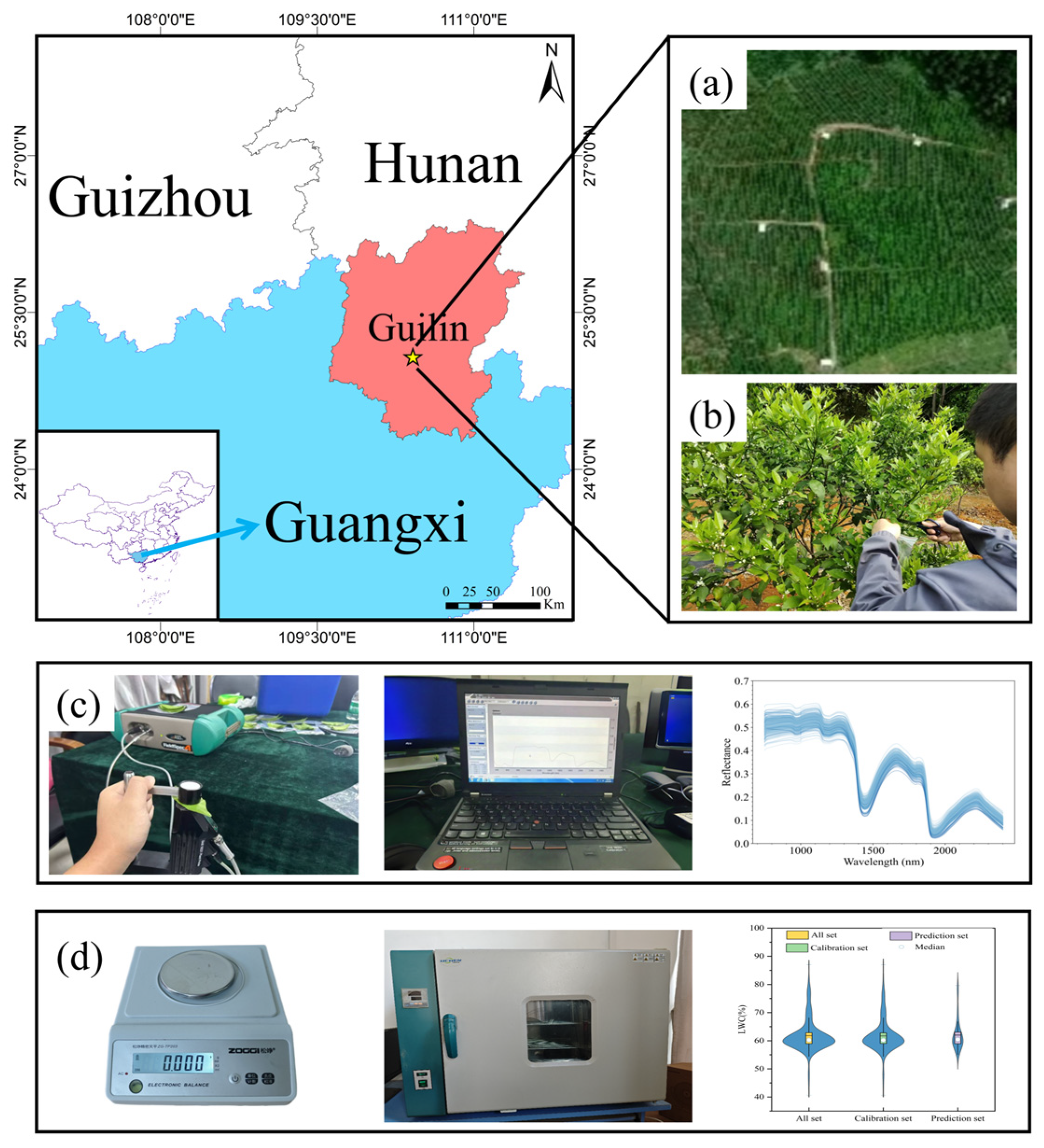
Guilin is located in the southwestern part of the Nanling Mountains, in the northeastern region of the Guangxi Zhuang Autonomous Region (25°16′30″ N, 110°33′28″ E), and is an important citrus-producing area in Guangxi. As shown in Figure 1a, this study selected the Citrus Cooperative Practice Base in Yanshan District, Guilin, as the experimental area. The selected region has a subtropical monsoon climate with distinct seasons, an annual average sunshine duration of approximately 1580 h, an average annual precipitation of approximately 1770 mm, and an average annual temperature of approximately 19 °C. The soil in the experimental area is red soil that is rich in nitrogen, phosphorus, potassium, and other essential mineral elements for fruit trees. These favourable climatic and soil conditions provide an optimal environment for the growth of citrus trees.
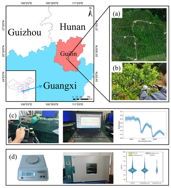
Figure 1.
(a) Aerial images of the study area. (b) Sample blade acquisition. (c) Hyperspectral data acquisition. (d) LWC data acquisition.
2.2. Data and Spectrum Acquisition
2.2.1. Sample Collection
The experimental data were collected on the morning of 8 April 2023, at the practical base of the Citrus Cooperative in Yanshan District, Guilin City, during the early fruit formation stage of seedless Wogan. During this stage, dynamic changes in leaf water content directly affect fruit growth and development, and their monitoring can prevent water imbalance-induced premature fruit drop or developmental retardation. To minimize environmental variation effects on the data and ensure the representativeness of leaf water content measurements, 60 healthy seedless Wogan trees were randomly selected as samples in the orchard. From each tree, five leaves were collected from each of the four cardinal directions (east, south, west, and north), spanning from the bottom to the top of the canopy (20 leaves per tree), resulting in 1200 leaves in total. Due to the low fresh weight of individual citrus leaves, separate weighing could be affected by electronic balance precision limitations and environmental disturbances. To more accurately reflect the water status across different orientations of the sample trees, five leaves from the same orientation were combined into 1 sample, yielding 240 samples in total. After collection, surface impurities on the leaves were immediately removed. The fresh weight of leaves was promptly measured, then the leaves were sealed in bags, labelled, stored in refrigerated containers, and rapidly transported to the laboratory for spectral and biochemical parameter measurements.
2.2.2. Spectral Data Collection
This study collected leaf hyperspectral data using a portable ASD (Analytical Spectral Devices, Boulder, CO, USA) spectrometer (Figure 1b). Prior to spectral data collection, the instrument was calibrated via a handheld leaf clip’s standard white reference panel (with approximately 100% spectral reflectance), and a white panel calibration was performed every 15 min during the measurements. To eliminate baseline drift errors, the ASD instrument was powered on and preheated for more than 30 min. Each leaf was placed flat in the clip to ensure a consistent detection area across all the samples, with measurements taken after the spectral curve stabilized on the display. To minimize noise and maximize the signal-to-noise ratio, 10 spectral curves were first collected for each leaf, and their average was calculated using ViewSpecPro_6_2 software to obtain the leaf’s hyperspectral reflectance data. Then, data from 5 leaves per sample were averaged again to generate representative spectral data for that sample. Finally, hyperspectral data from all 240 samples were uniformly saved as CSV files. The ASD spectrometer measures a spectral range from 350 to 2500 nm, with a sampling interval of 3 nm for the range of 350–1400 nm and 30 nm for the range of 1400–2500 nm. Since the 350–749 nm range is heavily influenced by leaf pigments (e.g., chlorophyll), removing this range reduces interference between pigments and water content, improving the model’s accuracy in reflecting water content [26]. Additionally, owing to strong noise interference in the 2400–2500 nm range [27], the final analysis retained 1651 valid bands in the 750–2400 nm range for further analysis.
2.2.3. Measured Water Content
As shown in Figure 1c, the collected citrus leaves were weighed using the precision electronic balance ZG-TP203 (Yongkang Songjing Trading Co., Ltd., Yongkang, China) with an accuracy of 0.001 g. The fresh weight (FW) of the leaves was measured immediately at the collection site. After completing the spectral reflectance measurements in the laboratory, the leaves were placed in the electric thermostatic drying oven 101-1BS (LICHEN, Shanghai LICHEN Instrument Technology Co., Ltd., Shanghai, China) preheated at 105 °C for 30 min for drying, and the drying oven was maintained at 80 °C until the weight of the leaves remained constant. Finally, the dry weight (DW) of the leaves was measured and recorded, and the LWC was calculated via Equation (1).
2.2.4. Dataset Division and Statistical Information Presentation
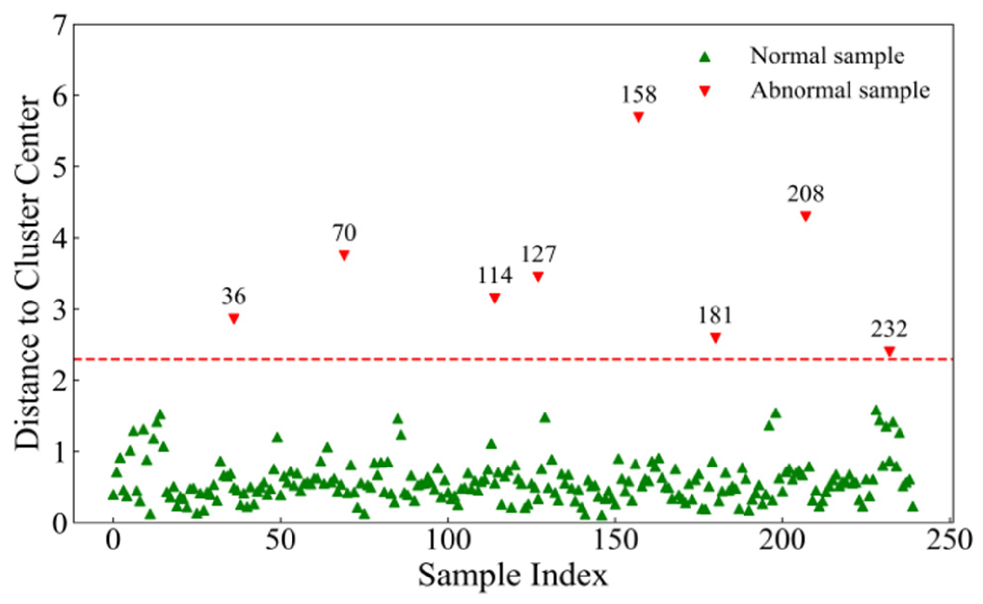
A total of 240 LWC samples were obtained during the experiment. To facilitate better modelling and analysis, the water content data were processed via the K-means clustering algorithm to detect outliers before further data handling. The number of cluster centres was set to 2, and the threshold was defined as the mean distance plus three times the standard deviation. As shown in Figure 2, 8 outlier samples were removed, leaving 232 valid samples. These samples were sorted on the basis of water content and divided into 10 layers. A stratified sampling method was applied at a ratio of 4:1, resulting in 185 samples for the modelling set and 47 samples for the prediction set. Table 1 presents the statistical data on the water content for the modelling set, prediction set, and total sample set. The modelling set covers the full range of maximum and minimum water content values, allowing the model to learn features across different water content levels. The means and standard deviations of the three data groups are relatively close, indicating that the data distribution is relatively concentrated yet exhibits some variability. This distribution helps the model learn both typical water content values and their fluctuations, thus improving prediction accuracy.
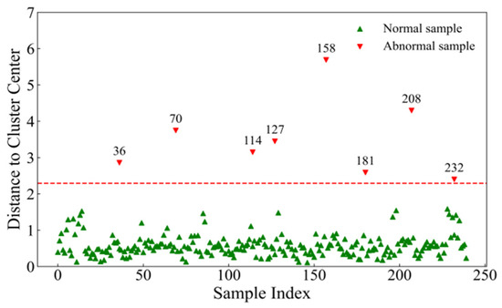
Figure 2.
Detection of abnormal results via K-means clustering.

Table 1.
LWC basic statistics of the modelling set, prediction set, and total sample.
2.3. Spectral Data Combinations
Spectral data are often affected by stray light, noise, and baseline drift, and preprocessing is critical for improving the signal-to-noise ratio, reducing errors, and enhancing data validity. Owing to the limitations of individual methods and the complexity of noise, a single preprocessing method is often insufficient to eliminate noise completely, and no universal standard preprocessing method exists that applies to all data [28]. Therefore, ensemble preprocessing has emerged as a solution, enhancing useful information in the data and improving model performance and stability through the combination of multiple methods. This study selected three mainstream preprocessing methods to explore an efficient and comprehensive ensemble approach. These methods include the 1st D for baseline correction, CWT for extracting multiscale features, and MSC for correcting scattering effects. Each preprocessing method targets different types of noise or bias, and combining them enables the extraction of more complementary information.
2.3.1. First Derivative
The first derivative (1st D) is an effective preprocessing method for addressing baseline drift and overlapping peaks [19,29]. It amplifies subtle differences between overlapping peaks, making the boundaries between peaks more distinct, thereby achieving effective separation and identification of overlapping peaks. Additionally, first derivative processing transforms the baseline drift into zero-value regions, correcting the baseline and enhancing data stability. In this study, to avoid amplifying high-frequency noise, the first derivative was computed via Savitzky–Golay (SG) convolution (with a window size of 5 and a polynomial order of 2). The SG filter is a sliding window filter based on polynomial least-squares fitting, which smooths the data while preserving high-frequency information, a crucial aspect for spectral analysis that requires retaining peak details.
2.3.2. Continuous Wavelet Transform
The continuous wavelet transform (CWT) offers significant advantages in processing high-dimensional data because of its unique time–frequency analysis capabilities [30]. Through CWT, hyperspectral data can be decomposed into wavelet coefficients at different scales, enabling analysis across different time–frequency points, effectively enhancing the discernibility of subtle spectral features while preserving key peak and shape information. The multiscale analysis of CWT is implemented via integral transformation, where the original signal is convolved with wavelet functions defined by various scales and translation parameters, as shown in Equation (2):
where is the scale factor (controlling the wavelet’s dilation), is the translation factor (controlling the wavelet’s movement along the time axis), represents the wavelet coefficients, which are functions of scale α and translation , is the original signal, and is the complex conjugate of the wavelet function .
In this study, since the hyperspectral characteristics of leaves resemble a Gaussian function [31], the “gaus5” wavelet from the Gaussian function family was selected as the mother wavelet. The original spectrum was decomposed into 10 scales, specifically 21, 22, …, 210. By comparing the Pearson correlation coefficients between the wavelet coefficients at different scales and the citrus LWC, the wavelet coefficients at scale 6 were ultimately chosen for use in this study.
2.3.3. Multiplicative Scatter Correction
Multiplicative scatter correction (MSC) effectively eliminates scattering effects in spectral data, bringing the spectral data closer to the true spectral response and improving the quality and reliability of the data [5,32]. Specifically, (1) the mean spectrum is calculated by averaging the spectral data of all samples (Equation (3)). (2) A linear regression is performed between each sample’s spectral data and the mean spectrum to obtain the linear regression coefficients ai and bi (Equation (4)). (3) The spectral data of each sample are corrected via the regression coefficients ai and bi (Equation (5)).
In these equations, is the number of samples, represents the spectral data of the sample, is the intercept, is the slope, and represents the corrected sample spectral data.
2.4. Development of the New EDPNet Network Based on the CNN Architecture
2.4.1. Multichannel Parallel Design of the New EDPNet Network
To fully exploit the spectral preprocessing combination information and achieve high-precision predictions of citrus LWC, this study builds on previous research showing that overly complex CNN architectures perform poorly in regression tasks [21,33]. Consequently, the simpler LeNet-5 architecture was selected and improved to develop the Ensemble Data Preprocessing Network (EDPNet) architecture. As shown in Figure 3, EDPNet uses a multichannel parallel design, where each channel corresponds to one type of spectral preprocessing data and includes a convolutional layer (Conv-1), a batch normalization layer (BatchNorm), and a max pooling layer (Pooling-1). These layers stack to extract features effectively from the original spectral data. The output features from all the parallel channels are fused through a concatenation layer (Concat), followed by another convolutional layer (Conv-2) and a max pooling layer (Pooling-2) for further learning. Finally, two fully connected layers and a linear activation function in the output layer establish the regression relationship between the spectral features and citrus LWC, which outputs the prediction results.
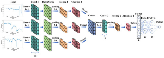
Figure 3.
New model architecture of EDPNet.
All the convolutional layers use a kernel size of 5 × 1, with a stride of 1. The max pooling layers have a pooling window size and stride of 2. Both fully connected layers have 16 neurons. On the basis of model evaluation metrics, the number of filters in the convolutional layers for each channel was set to 32, whereas the number of filters in the concatenated convolutional layer was set to 16. To capture the nonlinearities in the data, “ReLU” was selected as the activation function between layers (except for the output layer), which was based on a trial-and-error approach. Additionally, the weights of the layers were initialized via the “HeNormal” initializer. The model was trained via the Adam optimizer, and an automatic early stopping algorithm was employed to monitor the validation loss. If the validation loss did not improve by more than 10−5 for 50 consecutive epochs, the training was terminated.
All regression models were implemented in Python 3.9.18 via the Spyder IDE 5.1.5 environment, with all the 1D-CNN models built in TensorFlow 2.10.0 [34]. The experiments were run on a workstation equipped with an NVIDIA GPU (GeForce ® GTX 1660 SUPER; NVIDIA Corporation, Santa Clara, CA, USA), an Intel® Core™ i5-10400 CPU (Intel Corporation, Santa Clara, CA, USA; base frequency 2.90 GHz), and 16.0 GB of RAM. Owing to the inherent randomness in neural network training, slight variations in results may occur across different versions of TensorFlow during training on the GPU.
2.4.2. Attention Mechanism
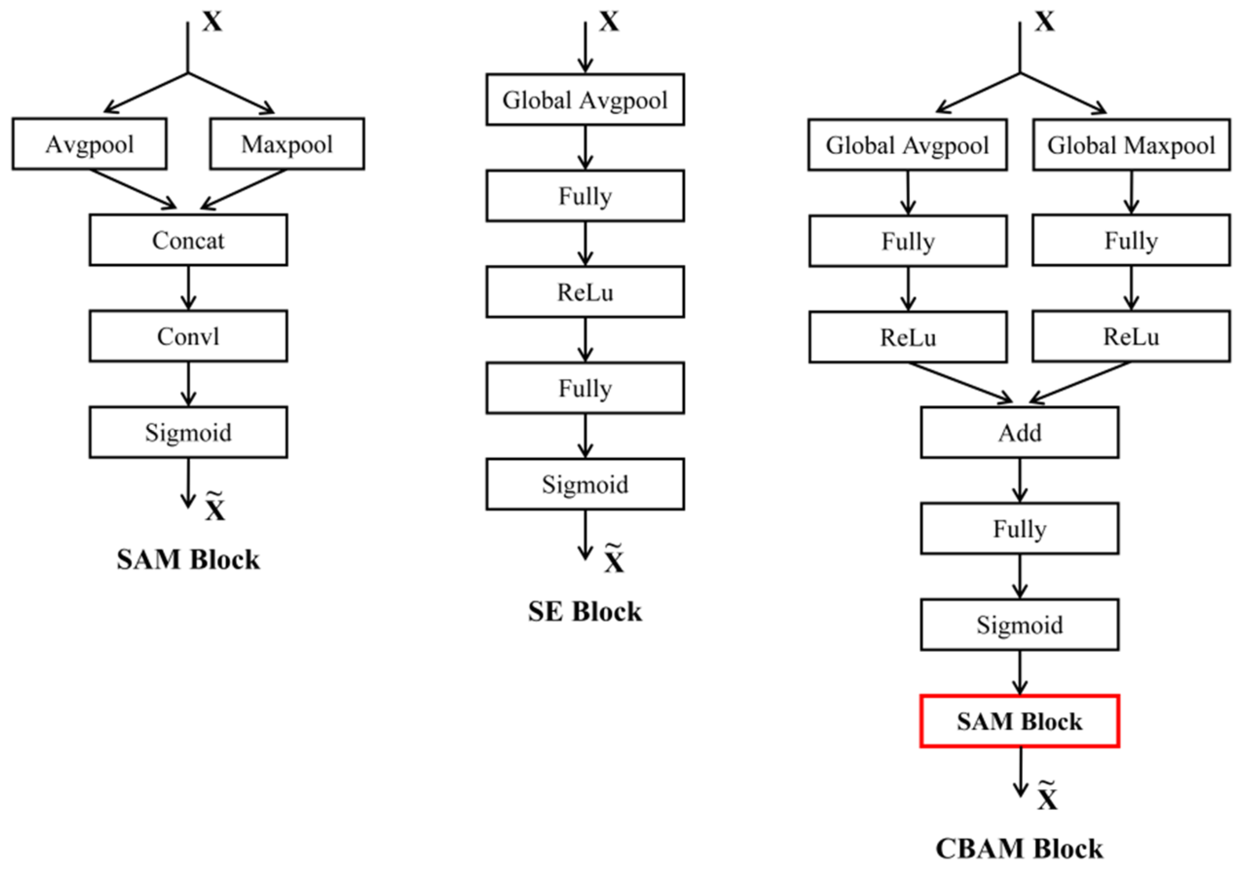
The core idea of the attention mechanism is to enable the network to “focus” on key features through a weighting method, thereby significantly improving the model’s performance in complex tasks. To explore the impact of the attention modules on model performance, three lightweight attention modules, whose positions within the model are shown in Figure 3, were selected and compared. The three modules are the channel attention module squeeze-and-excitation block (SE block) [35], the spatial attention module (SAM), and the hybrid module composed of the convolutional block attention module (CBAM) [36], which combines both channel and spatial attention.
These three attention modules enhance the model’s feature extraction through specific mechanisms. The SE block compresses information through global average pooling and calculates channel dependencies, adjusting the channel response weights. The SAM uses pooling operations to capture global spatial information, generating spatial attention maps to highlight important positions. CBAM combines both channel and spatial attention, first weighting the channels and then optimizing the spatial feature response. This study compares the performance of these modules in predicting citrus LWC and evaluates their effectiveness in enhancing the ability of CNNs to process spectral combination information. Figure 4 shows the basic structure of the three modules. In this experiment, certain adjustments were made to the modules to ensure that they effectively adapt to and process the input of one-dimensional hyperspectral data.

Figure 4.
Architecture of the SAM module (left), SE module (middle), and CBAM module (right). The SAM Block highlighted in red in the CBAM module is the SAM Block shown on the left. is the input feature, and is the weighted feature.
2.4.3. Model Feature Importance Analysis Method
The saliency map is a commonly used tool for visualizing the importance of model features, showing the contribution of input features to the model’s predictions and aiding in explaining the model’s decision-making process. Its principle is based on calculating the gradient of the output with respect to the input, identifying which features have the greatest impact on the result. The higher the gradient value, the greater the contribution of the feature to the prediction. This technique is widely used in image classification and has gradually been applied to multidimensional data analysis [37,38,39].
In this study, we modified the visualization method mentioned in the research by Xiao et al. to visualize the contribution of different preprocessing methods to the correct estimation by the model [21]. First, the CNN model was trained to predict citrus LWC values. Then, we calculated the prediction error rate via Equation (6):
Samples with an error rate less than 5% were considered “correctly predicted samples”. Saliency maps were generated on the basis of these “correctly predicted samples”, and the feature bands were ranked in descending order of absolute gradient values. Next, the top 10% of key feature wavelengths were selected from each “correctly predicted sample”, and the wavelengths were traced back to their corresponding preprocessing method. Finally, a contribution chart was plotted on the basis of the proportion of key feature wavelengths attributed to each preprocessing method, illustrating their respective contributions to the model.
2.5. Evaluation Metrics
In this study, the coefficient of determination (R2) and root mean square error (RMSE) were used to compare models and identify the best-performing model for all combination sets. R2 is a statistical measure used to quantify how well the predicted values fit the actual observed values. The closer the R2 value is to 1, the better the model’s predictions fit the actual observations. The RMSE is a statistical metric that measures the magnitude of the difference between the predicted values and the actual observed values. A smaller RMSE indicates smaller prediction errors. Overall, a higher R² and a lower RMSE are considered indicators of a good predictive model. R² and RMSE were evaluated via Equations (7) and (8), respectively:
where and represent the predicted and observed LWC values for the i-th citrus leaf, respectively, represents the mean of all observed LWC values, and represents the sample size. In this study, the RMSE units are consistent with leaf water content, both in %.
3. Results
3.1. Analysis of Spectral Curve Response Characteristics
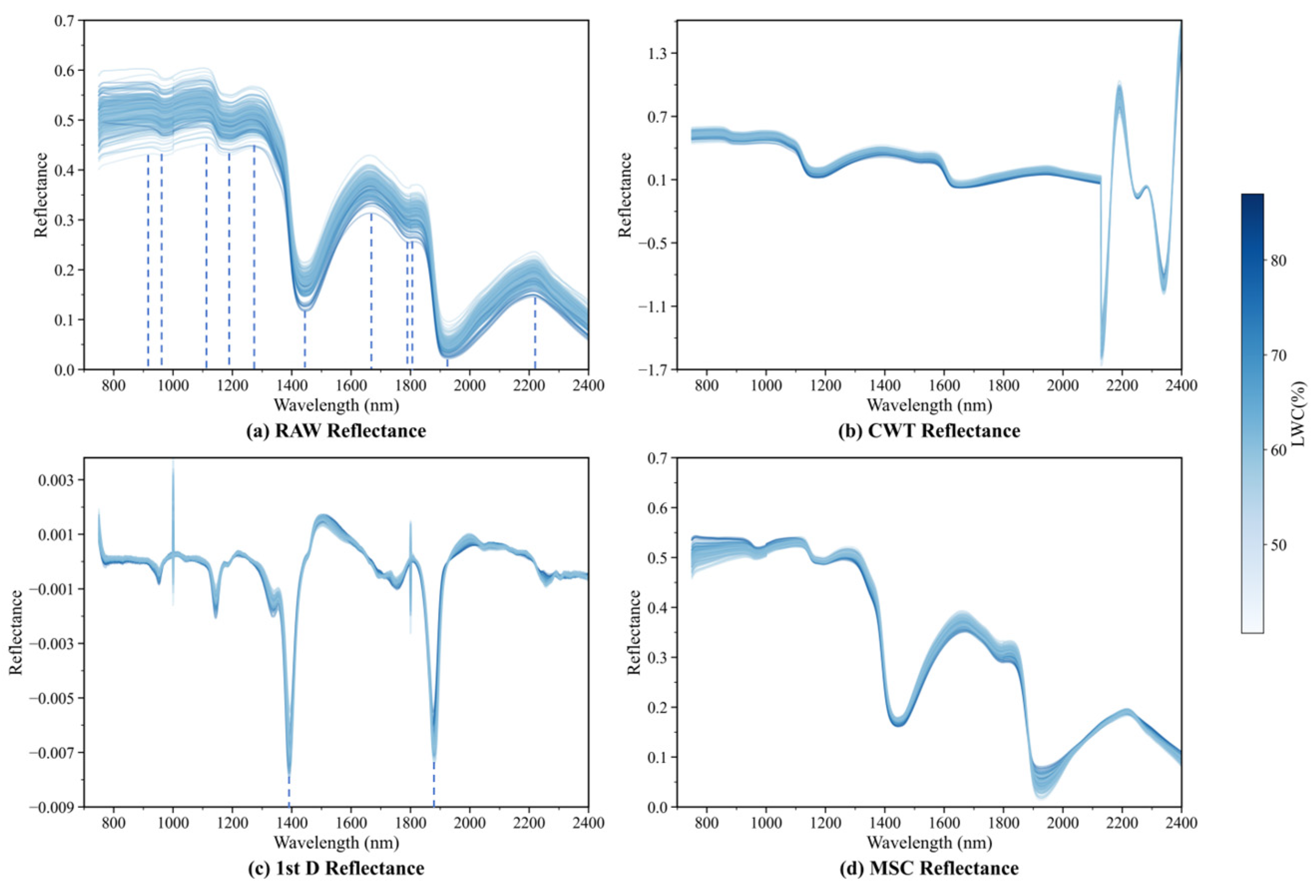
The raw spectral curves of 232 citrus leaf samples in the 750–2400 nm range are shown in Figure 5a, with the colour of the curves representing the corresponding LWC values (the darker the colour, the higher the LWC). As shown in Figure 5a, the raw reflectance spectra of different samples exhibit similar trends, with reflectance values ranging from 0.02 to 0.61. This phenomenon is primarily determined by the biochemical properties and structure of citrus leaves. Owing to the absorption of radiation by water, the LWC affects the spectral reflectance in the near-infrared (NIR) and shortwave infrared (SWIR) bands. In Figure 5a, the darker spectral curves generally exhibit lower reflectances, indicating that the LWC is the primary factor influencing the spectral reflectances in the NIR and SWIR bands. The raw spectra display six reflectance peaks (near 920, 1102, 1269, 1662, 1822, and 2217 nm) and five absorption troughs (near 969, 1194, 1443, 1794, and 1927 nm). Tucker’s research indicates that several wavelengths near these regions contain key information highly correlated with the LWC [40]. Specifically, the absorption peak at 969 nm may be attributed to the second overtone of O–H bonds [41], whereas the absorption peak at 1194 nm and the reflectance peak at 1269 nm are related to the second overtone of C–H stretching [42]. The peak at 1822 nm involves a combination of O–H and C–O stretching effects, whereas the reflectance peak at 2217 nm is associated with the second overtone of C–O stretching and a combination of N–H stretching and NH2 wagging [43].

Figure 5.
(a) Original spectral curves; (b) spectra after CWT processing; (c) spectra after 1st D processing; (d) spectra after MSC processing.
The spectral curves after the CWT, 1st D, and MSC preprocessing are shown in Figure 5b–d, respectively. These methods remove noise to varying degrees, resulting in smoother spectral curves. In particular, the 1st D-processed spectral curves feature two distinct troughs corresponding to the strong absorption troughs at 1443 nm and 1927 nm in the raw spectra, which are related to the first overtone of O–H stretching, revealing significant water absorption bands [44,45].
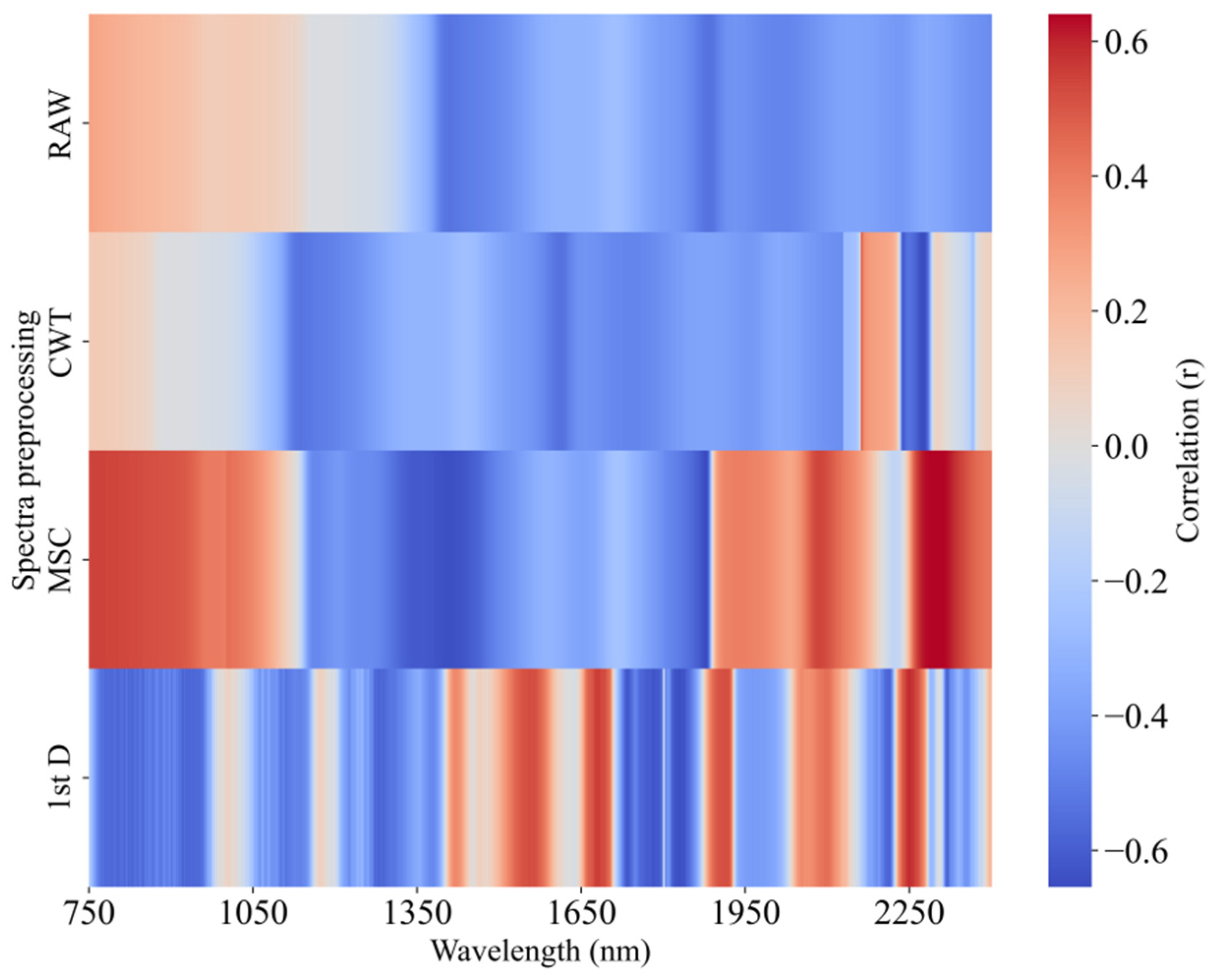
Figure 6 presents the Pearson correlation coefficient (r) heatmap between the wavelengths and LWC for both the raw and preprocessed data. In the raw spectra, the NIR band (750–1148 nm) is positively correlated with the LWC, which is consistent with findings from researchers such as El-Hendawy [46] and Liu [47]. In the 1149–2400 nm range, the reflectance shows a significant negative correlation with the LWC, especially near the 1390–1480 nm and 1860–1900 nm bands, with the strongest negative correlation occurring at 1884 nm (r = −0.541). After preprocessing, the correlation between the reflectance and LWC changed to varying degrees. The correlation trend after CWT preprocessing was similar to that of the raw spectrum in the 750–2130 nm range but with a noticeable shift towards shorter wavelengths, and a significantly different correlation pattern emerged after 2130 nm, with the maximum r value occurring at 2276 nm (r = −0.654). After MSC processing, the differences in spectra caused by varying scatter levels were eliminated, greatly enhancing the correlation between the reflectance and LWC, with the maximum r value occurring at 1877 nm (r = −0.651). The 1st D preprocessing also significantly improved the correlation, with an r value of −0.652 at 1829 nm. In the raw spectra, 567 wavelengths had a correlation coefficient greater than 0.4 with the LWC, while the numbers increased to 623, 988, and 829 after CWT, MSC, and 1st D preprocessing, respectively.
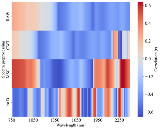
Figure 6.
Pearson correlation coefficient (r) heatmaps of the raw wavelength and pretreatment wavelength and LWC.
The results indicate that these three preprocessing methods extract different useful information from the raw spectra and effectively enhance the correlation between the reflectance and LWC. The contribution of the information derived from each preprocessing method to the high-precision prediction of citrus LWC still requires further analysis via neural network models.
3.2. Analysis of Spectral Combination Information
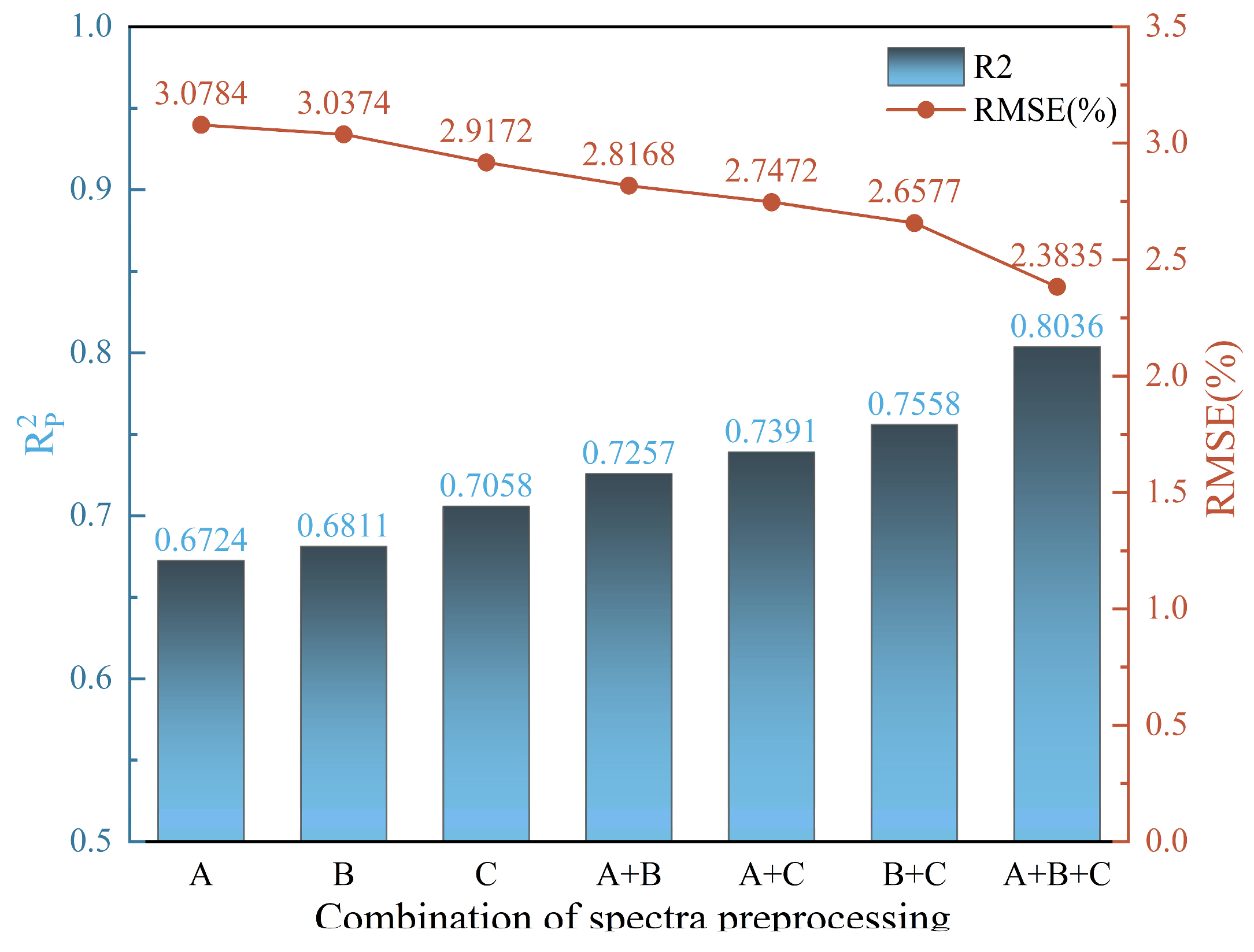
To explore the effects of different preprocessing methods and their combinations on model performance, seven CNN models were built via various combinations of spectral preprocessing methods. These models all employed the new architecture with identical parameter settings, and the best spectral preprocessing combination was determined by the optimal performance indicators, R2 and RMSE, on the prediction set. The final results are shown in Table 2. As illustrated in Figure 7, regardless of the preprocessing method, when the number of methods in the combination increased, the model’s accuracy improved. When the number of methods in the combination reached three, the CNN model performed best, with an R2 of 0.8036 and an RMSE of 2.3835 on the prediction set, representing a 13.86% improvement in R2 and an 18.29% reduction in RMSE compared with the best single preprocessing model (CWT). Among the dual preprocessing combinations, the CWT and MSC combination performed the best, with an R2 of 0.7558 and an RMSE of 2.6577 on the prediction set, demonstrating a notable improvement over single preprocessing methods, with R2 increasing by at least 7.08% and RMSE decreasing by 13.19%. A comparison of the three spectral preprocessing methods revealed that the CWT consistently performed well across different combinations, demonstrating its ability to improve model accuracy.
Table 2.
Model precision table of the combination of different spectral pretreatment methods.
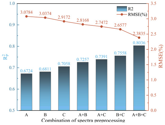
Figure 7.
R2 and RMSE of the model based on the spectral combination in the prediction set, where A represents the 1st D, B represents MSC, and C represents CWT.
Figure 8a illustrates the contribution proportions of each spectral preprocessing method in the three-method combination model, which were calculated via saliency maps. The results show that all three methods contributed significantly to the model’s accurate predictions, with the contributions ranked from highest to lowest as 1st D, MSC, and CWT, accounting for 38.6%, 32.5%, and 28.9%, respectively. Combined with the correlation analysis in Section 3.1, 1st D could extract more features that are highly correlated with citrus LWC and widely distributed from the raw spectra, effectively reducing redundancy. Although MSC extracted more highly correlated features, their concentration might limit information coverage. To further investigate the performance differences of preprocessing methods across various LWC levels, correctly predicted samples were divided into three ranges: low LWC (40% ≤ LWC < 60%), medium LWC (60% ≤ LWC < 75%), and high LWC (75% ≤ LWC < 90%). The contributions of each preprocessing method in different LWC ranges were then analysed. As shown in Figure 8b–d, 1 stD showed the highest contribution among all water content levels, especially in its contribution to high-water-content samples, which reached 46.4%, indicating its universal advantage in spectral baseline correction and moisture-related feature extraction. In the medium-LWC range, CWT’s contribution increased, approaching that of MSC. In the high-LWC range, CWT’s contribution further increased, surpassing that of MSC by 12.6%. This trend suggests that as leaf water content increases, CWT’s multiscale analysis capability may better adapt to the spectral signal complexity under high-water conditions. On the basis of the results of this experiment, subsequent experiments employed feature data from the combination of the CWT, MSC, and 1st D preprocessing methods.
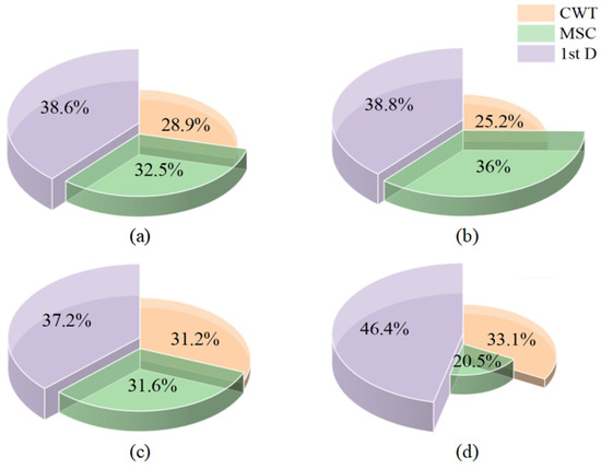
Figure 8.
Contribution analysis of three spectral preprocessing methods for correctly predicted samples based on saliency maps. (a) Correctly predicted samples; (b) low-water-content samples; (c) medium-water-content samples; (d) high-water-content samples.
3.3. Performance Comparison of Different CNN Architectures
The results above demonstrate that the combination of spectral information and a CNN can achieve high-accuracy predictions for citrus LWC. However, the key to CNN accuracy lies in the architecture, and different architectures can have varying effects on CNN model performance. Therefore, in this experiment, the performance of the custom-developed EDPNet architecture was evaluated against three classic CNN architectures for estimating LWC via spectral combination data. The layers and parameters of the three architectures are shown in Table 3. LeNet-5, AlexNet, and VGGNet were all adjusted and modified from their original architectures to accommodate one-dimensional input. In all the architectures, the ReLU activation function was paired with the “He_normal” weight initialization method. Except for the new architecture, where the input consisted of the stacked data from the three spectral preprocessing methods, the number of data samples did not increase, but the total number of variables increased from 1651 to 4953 (1651 × 3). To better compare it with EDPNet, LeNet-5 was configured with nearly the same parameters as EDPNet and included a batch normalization (BN) layer at the same positions.
Table 3.
Specific parameters of LeNet-5, AlexNet, and VGGNet architectures in the experiment.
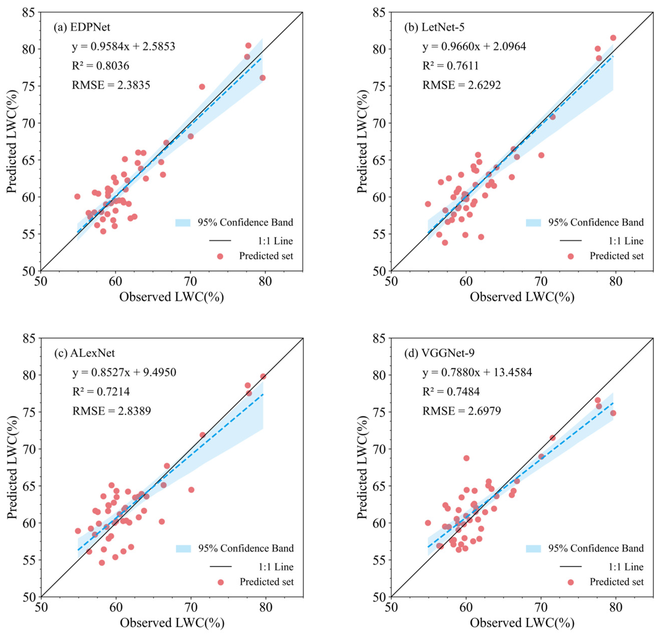
The accuracy results for the prediction sets of the models based on different CNN architectures are shown in Figure 9. In terms of accuracy, the best performer was the newly developed EDPNet, with an R2 of 0.8036 and an RMSE of 2.3835 on the prediction set, followed by the LeNet-5 architecture, with an R2 of 0.7611 and an RMSE of 2.6292. Among the two complex architectures, VGGNet (R2 = 0.7484, RMSE = 2.6979) performed better than AlexNet (R2 = 0.7214, RMSE = 2.8389). This difference may be related to the kernel size in the convolution layers, whereas AlexNet uses larger convolution kernels to increase the receptive field, which may lead to oversmoothing and the loss of local detail information. Combined with the results from Section 3.2, the prediction accuracy of the two complex architectures was lower than that of EDPNet on the basis of the combination of two preprocessing methods, indicating that these architectures failed to extract complementary information effectively from the combination data. Furthermore, under identical parameter and layer settings, EDPNet, which employs multichannel parallel convolution, outperformed LeNet-5, with R2 improving by 5.58% and RMSE decreasing by 9.35%, suggesting that multichannel parallel convolution is an effective approach that enhances model performance while reducing model complexity and computation. On the basis of these findings, this study identifies the multichannel parallel convolution-based EDPNet as the optimal CNN architecture for further analysis.
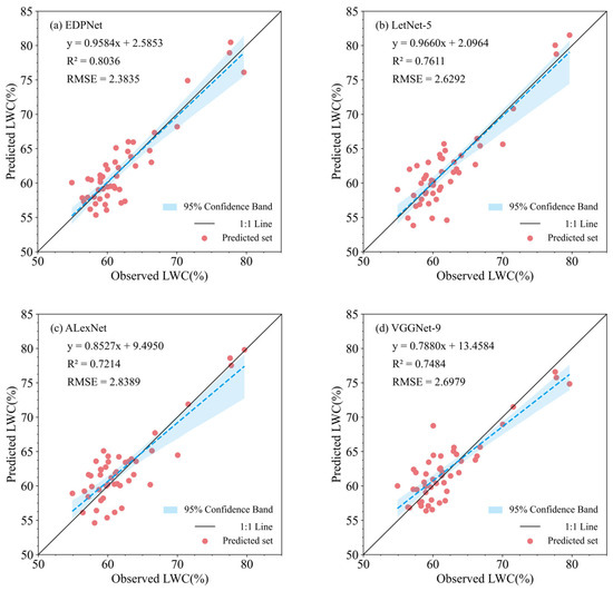
Figure 9.
Scatter diagram of the regression results of the model prediction set. (a) EDPNet. (b) LeNet-5. (c) AlexNet. (d) VGGNet.
3.4. Comparison of Attention Mechanisms
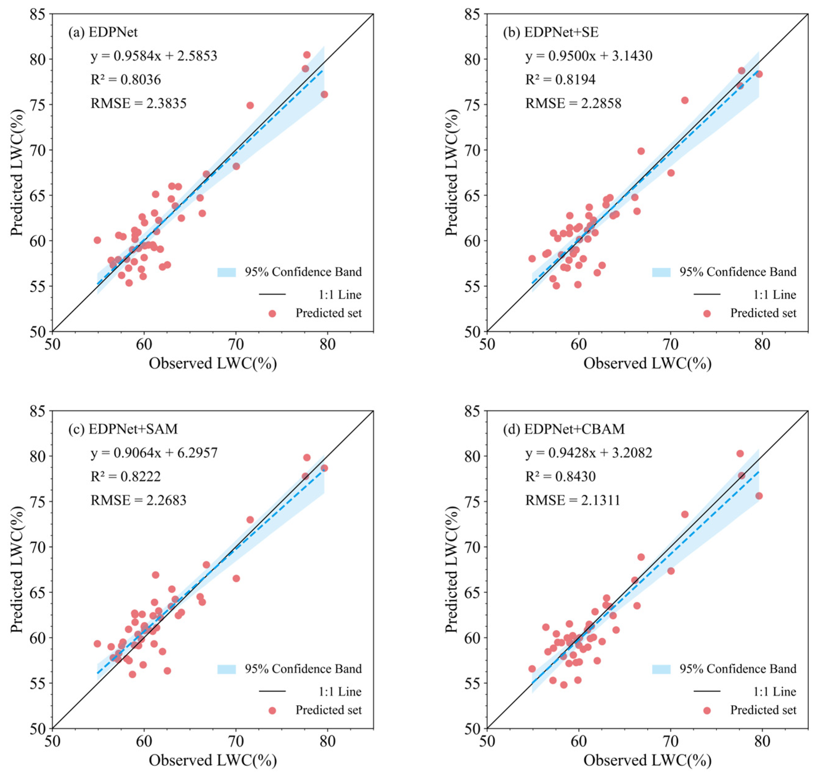
As shown in Figure 10, the LWC prediction results with and without attention modules demonstrate that the introduction of attention modules can enhance the performance of CNNs in estimating LWC to varying degrees. Specifically, introducing the spatial attention mechanism (SAM) (R² = 0.8222, RMSE = 2.2683) and the channel attention mechanism SE block (R² = 0.8194, RMSE = 2.2858) yielded good results in the LWC evaluation, with both models showing slight improvements in accuracy compared with the model without attention modules, with R² increasing by 1.58% to 1.86%. Notably, the EDPNet architecture, combined with the CBAM hybrid attention module, exhibited the best evaluation performance for LWC estimation (R² = 0.8430, RMSE = 2.1311). Compared with the model without attention modules, the prediction accuracy significantly improved, with an increase of 0.0394 in R². Additionally, compared with the other two attention modules, the CBAM hybrid attention module demonstrated an accuracy improvement of 2.08% to 2.36%. These results indicate that attention mechanisms have significant potential in processing large sets of features from spectral combinations, particularly the hybrid attention mechanism that combines both spatial and channel attention. This combination helps the model better leverage the complementary information in different spectral preprocessing data, thus improving the model’s performance in evaluating LWC.
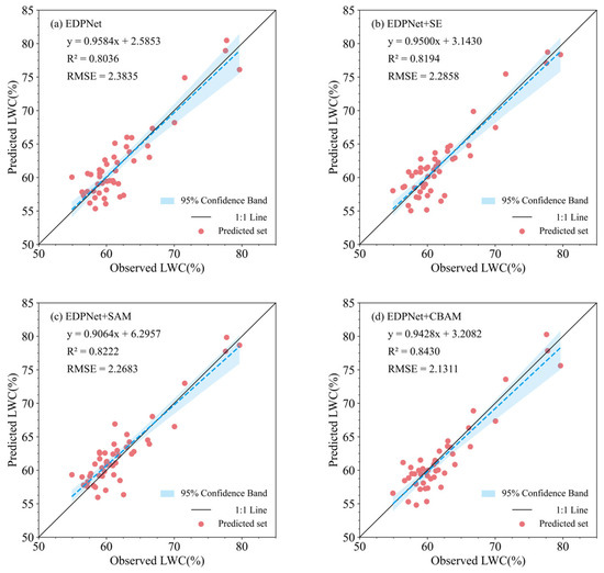
Figure 10.
Scatter diagram of the model regression results. (a) EDPNet. (b) Introduction of the SE module into the EDPNet model. (c) Introduction of the SAM module into the EDPNet model. (d) Introduction of the CBAM module into the EDPNet model.
4. Discussion
This study demonstrates that spectral preprocessing not only removes background information and noise but also preserves useful information [48]. Owing to the different principles and focuses of various preprocessing methods, they often complement each other. As shown in Figure 5, the raw spectral reflectances exhibit significant deviations, which are caused primarily by scattering effects, instrument errors, or operational inconsistencies. After MSC preprocessing, the standard deviation of the spectra significantly decreased, indicating that this method effectively corrects the spectral variations caused by scattering, making the data more consistent and more accurately reflecting the true spectral response [49]. Additionally, the spectra processed by the CWT and 1st D showed that random noise between samples was effectively eliminated. Specifically, the 1st D enhances subtle changes in the spectra by calculating the derivative, which is particularly important for identifying overlapping peaks and improving the spectral resolution [50]. CWT, with its multiscale analysis capability, can extract local features at different resolutions, better capturing key information in complex signals. The modelling results indicate that combining preprocessing methods that target different objectives improved model accuracy, which demonstrates that combining preprocessing information with a CNN is an automatic and efficient way of extracting spectral information. The saliency map analysis results show that all three preprocessing methods contributed to accurate modelling, synergistically improving model performance and further confirming that these methods offer complementary information. This conclusion aligns with the findings of Mishra et al. [11], who suggested that “a single preprocessing method is insufficient to eliminate all noise effects, and combining multiple methods can enhance model accuracy.”
In terms of model selection, CNNs are essentially multilayer perceptrons that can automatically learn the mapping relationship between raw data and sample labels [51], performing dimensionality reduction on feature data without manual feature engineering. Owing to their superior performance and strong generalization ability, CNNs have been widely used in the quantitative estimation of crop biochemical parameters [20,52]. However, there is no consensus on the optimal CNN architecture for the quantitative prediction of citrus LWC. To fully exploit the potential of spectral combination information, this study developed a new model, EDPNet, which is based on the classic LeNet-5 architecture, and compared it with three other classic architectures. The results show that, compared with the two simpler architectures, AlexNet and VGGNet underperformed on the prediction set, suggesting that network complexity is not always the key determinant of model superiority. Similarly, a study by Xiao et al. revealed that complex network structures do not necessarily suit spectral data processing [21]. Moreover, a comparison of AlexNet and VGGNet reveals that while larger convolution kernels can expand the model’s receptive field, they may also cause excessive smoothing, leading to a loss of local detail. The improved EDPNet outperforms LeNet-5, demonstrating that employing multichannel convolution is an effective strategy to enhance model performance. This aligns with the findings of Rehman et al. [53], whose DeepRWC model utilized parallel convolutional groups (Inception modules) to directly extract raw spectral features, significantly improving feature learning capability. While retaining this advantage, EDPNet simplifies the network architecture and integrates preprocessed data, reducing reliance on raw data quality and further optimizing computational efficiency. Experimental results demonstrate that EDPNet significantly improves feature learning efficiency while maintaining a lightweight architecture by integrating multispectral preprocessed data, and its superior performance in citrus LWC prediction highlights the model’s application potential.
Furthermore, this study introduced attention mechanisms and reported that models incorporating attention modules achieved improved accuracy, further leveraging the advantages of spectral preprocessing combinations. This finding is consistent with previous studies on crop biochemical parameter prediction, where 1D-CNNs combined with attention mechanisms demonstrated excellent performance [22,24]. The study by Ye et al. also showed that attention mechanisms can effectively highlight key wavelength information, and their proposed deep learning model exhibited higher prediction accuracy and robustness than traditional models did, which aligns with our results [25]. In the comparative experiment of the attention mechanism in this study, the SE module dynamically adjusts channel weights through “squeezing” and “stimulating” operations, whereas the SAM module focuses on spatial dimensional features. There is little difference between the two models in improving model performance, and both can effectively enhance the model to capture the dynamic response between the spectrum and citrus LWC and significantly improve the estimation accuracy on the prediction set. However, the CBAM module combines the attention mechanism of the channel and spatial dimensions, which not only optimizes the channel weight but also strengthens the spatial feature expression, thus improving the model performance in multiple dimensions. As a result, it performs best among the three attention mechanisms.
5. Conclusions
This study, which was conducted at the Citrus Cooperative Practice Base in Yanshan District, Guilin, China, employed three spectral preprocessing methods—MSC, CWT, and 1st D—along with the newly developed EDPNet model to validate the feasibility of using spectral combination information to overcome the limitations of individual preprocessing methods. This study also analysed the performance and strengths of different CNN architectures in integrating spectral combination information and explored the impact of various attention mechanisms on the accuracy of citrus LWC prediction. The main conclusions are as follows: (1) All three preprocessing methods enhance the correlation between raw spectra and LWC, and combining preprocessing methods with different focal points effectively improves model performance. (2) The newly developed EDPNet model, combined with spectral information, achieves high-precision predictions of citrus LWC (R2 = 0.8036, RMSE = 2.3835), indicating that the multichannel parallel network structure has significant potential for integrating spectral combination information. (3) Introducing attention mechanisms into EDPNet significantly improves prediction performance, with the CBAM hybrid attention module providing the greatest enhancement (R2 = 0.8430, RMSE = 2.1311), resulting in a 4.9% increase in R2 and a 10.59% decrease in RMSE compared with those of the original model.
This study developed a lightweight model for predicting citrus leaf water content, providing a technical reference for orchard digital management. The experimental results demonstrate that this model shows promising potential for identifying leaf water status, making it a foundational tool for smart orchard management. Future research could integrate deep transfer learning to extend the model to UAV remote sensing platforms, enabling large-scale canopy spectral data acquisition for orchard water dynamic monitoring systems and optimized irrigation decision-making. Additionally, the proposed architectural design can be adapted through parameter optimization to detect key biochemical indicators such as chlorophyll content, offering data support for intelligent orchard monitoring systems.
Author Contributions
Conceptualization, S.D. and X.R.; Methodology, S.D. and X.R.; Software, W.Z., X.Q. and Z.M.; Formal analysis, S.D. and X.R.; Validation, X.Y. and Z.M.; Funding acquisition, S.D.; Investigation, W.Z., X.Q. and Y.S.; Resources, X.R. and S.D.; Data curation, W.Z., Y.S. and X.Y.; Writing—original draft preparation, S.D. and X.R.; Writing—review and editing, S.D. and X.R.; Visualization, S.D.; Supervision, S.D., X.Q. and Z.M.; Project administration, S.D. All authors have read and agreed to the published version of the manuscript.
Funding
This study was supported by the Natural Science Foundation of Guangxi (No. 2023JJA150097); the Natural Science Foundation of Fujian Province (No. 2023J01957), the Guilin City Science Research and Technology Development Plan Project (No. 20230120-13).
Data Availability Statement
The data are part of an ongoing study. Data will be made available on request.
Conflicts of Interest
This manuscript has no conflicts of interest to declare.
References
- Shafqat, W.; Mazrou, Y.S.A.; Nehela, Y.; Ikram, S.; Bibi, S.; Naqvi, S.A.; Hameed, M.; Jaskani, M.J. Effect of Three Water Regimes on the Physiological and Anatomical Structure of Stem and Leaves of Different Citrus Rootstocks with Distinct Degrees of Tolerance to Drought Stress. Horticulturae 2021, 7, 554. [Google Scholar] [CrossRef]
- Gonzalez-Dugo, V.; Zarco-Tejada, P.J.; Fereres, E. Applicability and limitations of using the crop water stress index as an indicator of water deficits in citrus orchards. Agric. For. Meteorol. 2014, 198, 94–104. [Google Scholar] [CrossRef]
- Junttila, S.; Hölttä, T.; Saarinen, N.; Kankare, V.; Yrttimaa, T.; Hyyppä, J.; Vastaranta, M. Close-range hyperspectral spectroscopy reveals leaf water content dynamics. Remote Sens. Environ. 2022, 277, 113071. [Google Scholar] [CrossRef]
- Knipling, E.B. Physical and physiological basis for the reflectance of visible and near-infrared radiation from vegetation. Remote Sens. Environ. 1970, 1, 155–159. [Google Scholar] [CrossRef]
- Zhang, L.; Zhou, Z.; Zhang, G.; Meng, Y.; Chen, B.; Wang, Y. Monitoring the leaf water content and specific leaf weight of cotton (Gossypium hirsutum L.) in saline soil using leaf spectral reflectance. Eur. J. Agron. 2012, 41, 103–117. [Google Scholar] [CrossRef]
- Kong, Y.; Liu, Y.; Geng, J.; Huang, Z. Pixel-Level Assessment Model of Contamination Conditions of Composite Insulators Based on Hyperspectral Imaging Technology and a Semi-Supervised Ladder Network. IEEE Trans. Dielectr. Electr. Insul. 2023, 30, 326–335. [Google Scholar] [CrossRef]
- Zhao, R.; An, L.; Tang, W.; Gao, D.; Qiao, L.; Li, M.; Sun, H.; Qiao, J. Deep learning assisted continuous wavelet transform-based spectrogram for the detection of chlorophyll content in potato leaves. Comput. Electron. Agric. 2022, 195, 106802. [Google Scholar] [CrossRef]
- He, R.; Li, H.; Qiao, X.; Jiang, J. Using wavelet analysis of hyperspectral remote-sensing data to estimate canopy chlorophyll content of winter wheat under stripe rust stress. Int. J. Remote Sens. 2018, 39, 4059–4076. [Google Scholar] [CrossRef]
- Liu, N.; Xing, Z.; Zhao, R.; Qiao, L.; Li, M.; Liu, G.; Sun, H. Analysis of Chlorophyll Concentration in Potato Crop by Coupling Continuous Wavelet Transform and Spectral Variable Optimization. Remote Sens. 2020, 12, 2826. [Google Scholar] [CrossRef]
- Yu, G.; Li, H.; Li, Y.; Hu, Y.; Wang, G.; Ma, B.; Wang, H. Multiscale Deepspectra Network: Detection of Pyrethroid Pesticide Residues on the Hami Melon. Foods 2023, 12, 1742. [Google Scholar] [CrossRef]
- Mishra, P.; Roger, J.M.; Marini, F.; Biancolillo, A.; Rutledge, D.N. Parallel pre-processing through orthogonalization (PORTO) and its application to near-infrared spectroscopy. Chemom. Intell. Lab. Syst. 2021, 212, 104190. [Google Scholar] [CrossRef]
- Roger, J.-M.; Biancolillo, A.; Marini, F. Sequential preprocessing through ORThogonalization (SPORT) and its application to near infrared spectroscopy. Chemom. Intell. Lab. Syst. 2020, 199, 103975. [Google Scholar] [CrossRef]
- Bian, X.; Wang, K.; Tan, E.; Diwu, P.; Zhang, F.; Guo, Y. A selective ensemble preprocessing strategy for near-infrared spectral quantitative analysis of complex samples. Chemom. Intell. Lab. Syst. 2020, 197, 103916. [Google Scholar] [CrossRef]
- Nazarloo, A.S.; Sharabiani, V.R.; Gilandeh, Y.A.; Taghinezhad, E.; Szymanek, M. Evaluation of Different Models for Non-Destructive Detection of Tomato Pesticide Residues Based on Near-Infrared Spectroscopy. Sensors 2021, 21, 3032. [Google Scholar] [CrossRef]
- Sun, Q.; Gu, X.; Chen, L.; Qu, X.; Zhang, S.; Zhou, J.; Pan, Y. Hyperspectral estimation of maize (Zea mays L.) yield loss under lodging stress. Field Crops Res. 2023, 302, 109042. [Google Scholar] [CrossRef]
- Barman, U. Deep Convolutional neural network (CNN) in tea leaf chlorophyll estimation: A new direction of modern tea farming in Assam, India. J. Appl. Nat. Sci. 2021, 13, 1059–1064. [Google Scholar] [CrossRef]
- Kattenborn, T.; Leitloff, J.; Schiefer, F.; Hinz, S. Review on Convolutional Neural Networks (CNN) in vegetation remote sensing. ISPRS J. Photogramm. Remote Sens. 2021, 173, 24–49. [Google Scholar] [CrossRef]
- Li, S.; Song, Q.; Liu, Y.; Zeng, T.; Liu, S.; Jie, D.; Wei, X. Hyperspectral imaging-based detection of soluble solids content of loquat from a small sample. Postharvest Biol. Technol. 2023, 204, 112454. [Google Scholar] [CrossRef]
- Li, Y.; Ma, B.; Li, C.; Yu, G. Accurate prediction of soluble solid content in dried Hami jujube using SWIR hyperspectral imaging with comparative analysis of models. Comput. Electron. Agric. 2022, 193, 106655. [Google Scholar] [CrossRef]
- Shi, S.; Xu, L.; Gong, W.; Chen, B.; Chen, B.; Qu, F.; Tang, X.; Sun, J.; Yang, J. A convolution neural network for forest leaf chlorophyll and carotenoid estimation using hyperspectral reflectance. Int. J. Appl. Earth Obs. Geoinf. 2022, 108, 102719. [Google Scholar] [CrossRef]
- Xiao, Q.; Tang, W.; Zhang, C.; Zhou, L.; Feng, L.; Shen, J.; Yan, T.; Gao, P.; He, Y.; Wu, N. Spectral Preprocessing Combined with Deep Transfer Learning to Evaluate Chlorophyll Content in Cotton Leaves. Plant Phenomics 2022, 2022, 9813841. [Google Scholar] [CrossRef] [PubMed]
- Yu, S.; Fan, J.; Lu, X.; Wen, W.; Shao, S.; Liang, D.; Yang, X.; Guo, X.; Zhao, C. Deep learning models based on hyperspectral data and time-series phenotypes for predicting quality attributes in lettuces under water stress. Comput. Electron. Agric. 2023, 211, 108034. [Google Scholar] [CrossRef]
- Niu, Z.; Zhong, G.; Yu, H. A review on the attention mechanism of deep learning. Neurocomputing 2021, 452, 48–62. [Google Scholar] [CrossRef]
- Weng, S.; Han, K.; Chu, Z.; Zhu, G.; Liu, C.; Zhu, Z.; Zhang, Z.; Zheng, L.; Huang, L. Reflectance images of effective wavelengths from hyperspectral imaging for identification of Fusarium head blight-infected wheat kernels combined with a residual attention convolution neural network. Comput. Electron. Agric. 2021, 190, 106483. [Google Scholar] [CrossRef]
- Ye, Z.; Tan, X.; Dai, M.; Chen, X.; Zhong, Y.; Zhang, Y.; Ruan, Y.; Kong, D. A hyperspectral deep learning attention model for predicting lettuce chlorophyll content. Plant Methods 2024, 20, 22. [Google Scholar] [CrossRef]
- Cotrozzi, L.; Couture, J.J.; Cavender-Bares, J.; Kingdon, C.C.; Fallon, B.; Pilz, G.; Pellegrini, E.; Nali, C.; Townsend, P.A. Using foliar spectral properties to assess the effects of drought on plant water potential. Tree Physiol. 2017, 37, 1582–1591. [Google Scholar] [CrossRef] [PubMed]
- Zhang, Z.; Ding, J.; Wang, J.; Ge, X. Prediction of soil organic matter in northwestern China using fractional-order derivative spectroscopy and modified normalized difference indices. Catena 2020, 185, 104257. [Google Scholar] [CrossRef]
- Mishra, P.; Biancolillo, A.; Roger, J.M.; Marini, F.; Rutledge, D.N. New data preprocessing trends based on ensemble of multiple preprocessing techniques. TrAC Trends Anal. Chem. 2020, 132, 116045. [Google Scholar] [CrossRef]
- Xiao, B.; Li, S.; Dou, S.; He, H.; Fu, B.; Zhang, T.; Sun, W.; Yang, Y.; Xiong, Y.; Shi, J.; et al. Comparison of leaf chlorophyll content retrieval performance of citrus using FOD and CWT methods with field-based full-spectrum hyperspectral reflectance data. Comput. Electron. Agric. 2024, 217, 108559. [Google Scholar] [CrossRef]
- Li, L.; Geng, S.; Lin, D.; Su, G.; Zhang, Y.; Chang, L.; Ji, Y.; Wang, Y.; Wang, L. Accurate modeling of vertical leaf nitrogen distribution in summer maize using in situ leaf spectroscopy via CWT and PLS-based approaches. Eur. J. Agron. 2022, 140, 126607. [Google Scholar] [CrossRef]
- Koger, C. Wavelet analysis of hyperspectral reflectance data for detecting pitted morningglory (Ipomoea lacunosa) in soybean (Glycine max). Remote Sens. Environ. 2003, 86, 108–119. [Google Scholar] [CrossRef]
- Xiang, Y.; Chen, Q.; Su, Z.; Zhang, L.; Chen, Z.; Zhou, G.; Yao, Z.; Xuan, Q.; Cheng, Y. Deep Learning and Hyperspectral Images Based Tomato Soluble Solids Content and Firmness Estimation. Front. Plant Sci. 2022, 13, 860656. [Google Scholar] [CrossRef] [PubMed]
- Prilianti, K.R.; Setiyono, E.; Kelana, O.H.; Brotosudarmo, T.H.P. Deep chemometrics for nondestructive photosynthetic pigments prediction using leaf reflectance spectra. Inf. Process. Agric. 2021, 8, 194–204. [Google Scholar] [CrossRef]
- Abadi, M.; Barham, P.; Chen, J.; Chen, Z.; Davis, A.; Dean, J.; Devin, M.; Ghemawat, S.; Irving, G.; Isard, M.; et al. TensorFlow: A system for Large-Scale machine learning. In Proceedings of the 12th USENIX Symposium on Operating Systems Design and Implementation (OSDI 16), Savannah, GA, USA, 2–4 November 2016; pp. 265–283. [Google Scholar] [CrossRef]
- Hu, J.; Shen, L.; Albanie, S.; Sun, G.; Wu, E. Squeeze-and-Excitation Networks. IEEE Trans. Pattern Anal. Mach. Intell. 2020, 42, 2011–2023. [Google Scholar] [CrossRef]
- Woo, S.; Park, J.; Lee, J.-Y.; Kweon, I.S. CBAM: Convolutional Block Attention Module. In Proceedings of the European Conference on Computer Vision (ECCV), Munich, Germany, 8–14 September; 8–14 September 2018. [Google Scholar] [CrossRef]
- Alqaraawi, A.; Schuessler, M.; Weiß, P.; Costanza, E.; Berthouze, N. Evaluating saliency map explanations for convolutional neural networks. In Proceedings of the 25th International Conference on Intelligent User Interfaces, Cagliari, Italy, 17–20 March; 17–20 March 2020. [Google Scholar] [CrossRef]
- Feng, L.; Wu, B.; He, Y.; Zhang, C. Hyperspectral Imaging Combined With Deep Transfer Learning for Rice Disease Detection. Front. Plant Sci. 2021, 12, 693521. [Google Scholar] [CrossRef]
- Su, Z.; Zhang, C.; Yan, T.; Zhu, J.; Zeng, Y.; Lu, X.; Gao, P.; Feng, L.; He, L.; Fan, L. Application of Hyperspectral Imaging for Maturity and Soluble Solids Content Determination of Strawberry With Deep Learning Approaches. Front. Plant Sci. 2021, 12, 736334. [Google Scholar] [CrossRef]
- Tucker, C.J. Remote sensing of leaf water content in the near infrared. Remote Sens. Environ. 1980, 10, 23–32. [Google Scholar] [CrossRef]
- Leiva-Valenzuela, G.A.; Lu, R.; Aguilera, J.M. Prediction of firmness and soluble solids content of blueberries using hyperspectral reflectance imaging. J. Food Eng. 2013, 115, 91–98. [Google Scholar] [CrossRef]
- Dong, J.; Guo, W. Nondestructive Determination of Apple Internal Qualities Using Near-Infrared Hyperspectral Reflectance Imaging. Food Anal. Methods 2015, 8, 2635–2646. [Google Scholar] [CrossRef]
- Türker-Kaya, S.; Huck, C. A Review of Mid-Infrared and Near-Infrared Imaging: Principles, Concepts and Applications in Plant Tissue Analysis. Molecules 2017, 22, 168. [Google Scholar] [CrossRef]
- Kamruzzaman, M.; ElMasry, G.; Sun, D.-W.; Allen, P. Prediction of some quality attributes of lamb meat using near-infrared hyperspectral imaging and multivariate analysis. Anal. Chim. Acta 2012, 714, 57–67. [Google Scholar] [CrossRef] [PubMed]
- Siedliska, A.; Baranowski, P.; Zubik, M.; Mazurek, W.; Sosnowska, B. Detection of fungal infections in strawberry fruit by VNIR/SWIR hyperspectral imaging. Postharvest Biol. Technol. 2018, 139, 115–126. [Google Scholar] [CrossRef]
- El-Hendawy, S.E.; Al-Suhaibani, N.A.; Elsayed, S.; Hassan, W.M.; Dewir, Y.H.; Refay, Y.; Abdella, K.A. Potential of the existing and novel spectral reflectance indices for estimating the leaf water status and grain yield of spring wheat exposed to different irrigation rates. Agric. Water Manag. 2019, 217, 356–373. [Google Scholar] [CrossRef]
- Liu, S.; Peng, Y.; Du, W.; Le, Y.; Li, L. Remote Estimation of Leaf and Canopy Water Content in Winter Wheat with Different Vertical Distribution of Water-Related Properties. Remote Sens. 2015, 7, 4626–4650. [Google Scholar] [CrossRef]
- Qiao, L.; Mu, Y.; Lu, B.; Tang, X. Calibration Maintenance Application of Near-infrared Spectrometric Model in Food Analysis. Food Rev. Int. 2021, 39, 1628–1644. [Google Scholar] [CrossRef]
- Isaksson, T.; Næs, T. The Effect of Multiplicative Scatter Correction (MSC) and Linearity Improvement in NIR Spectroscopy. Appl. Spectrosc. 1988, 42, 1273–1284. [Google Scholar] [CrossRef]
- Zimmermann, B.; Kohler, A. Optimizing Savitzky–Golay Parameters for Improving Spectral Resolution and Quantification in Infrared Spectroscopy. Appl. Spectrosc. 2013, 67, 892–902. [Google Scholar] [CrossRef]
- Moghimi, A.; Yang, C.; Anderson, J.A. Aerial hyperspectral imagery and deep neural networks for high-throughput yield phenotyping in wheat. Comput. Electron. Agric. 2020, 172, 105299. [Google Scholar] [CrossRef]
- Zhang, C.; Li, C.; He, M.; Cai, Z.; Feng, Z.; Qi, H.; Zhou, L. Leaf water content determination of oilseed rape using near-infrared hyperspectral imaging with deep learning regression methods. Infrared Phys. Technol. 2023, 134, 104921. [Google Scholar] [CrossRef]
- Rehman, T.U.; Ma, D.; Wang, L.; Zhang, L.; Jin, J. Predictive spectral analysis using an end-to-end deep model from hyperspectral images for high-throughput plant phenotyping. Comput. Electron. Agric. 2020, 177, 105713. [Google Scholar] [CrossRef]


Disclaimer/Publisher’s Note: The statements, opinions and data contained in all publications are solely those of the individual author(s) and contributor(s) and not of MDPI and/or the editor(s). MDPI and/or the editor(s) disclaim responsibility for any injury to people or property resulting from any ideas, methods, instructions or products referred to in the content. |
© 2025 by the authors. Licensee MDPI, Basel, Switzerland. This article is an open access article distributed under the terms and conditions of the Creative Commons Attribution (CC BY) license (https://creativecommons.org/licenses/by/4.0/).