Multi-Band-Image Based Detection of Apple Surface Defect Using Machine Vision and Deep Learning

Abstract

Accurate surface defect extraction of apples is critical for their quality inspection and marketing purposes. Using multi-band images, this study proposes a detection method for apple surface defects with a combination of machine vision and deep learning. Five single bands, 460, 522, 660, 762, and 842 nm, were selected within the visible and near-infrared. By using a near-infrared industrial camera with optical filters, five single-band images of an apple could be obtained. To achieve higher accuracy of defect extraction, an improved U-Net was designed based on the original U-Net network structure. More specially, the partial original convolutions were replaced by dilated convolutions with different dilated rates, and an attention mechanism was added. The loss function was also redesigned during the training process. Then the traditional algorithm, the trained U-Net and the trained improved U-Net were used to extract defects of apples in the test set. Following that, the performances of the three methods were compared with that of the manual extraction. The results show that the near-infrared band is better than the visible band for defects with insignificant features. Additionally, the improved U-Net is better than the U-Net and the traditional algorithm for small defects and defects with irregular edges. On the test set, for single-band images at 762 nm, the improved U-Net had the best defect extraction with an mIoU (mean intersection over union) and mF1-score of 91% and 95%, respectively.

1. Introduction

Benefiting from their rich nutritious and sweet taste, apples have been one of the most popular fruits. However, during the process of growing, picking, transporting, and storing apples, defects and damages inevitably occur, which will affect their taste and price. Therefore, the detection of surface defects on apples before picking and marketing is quite important for the implementation of apple grading and automatic sorting. Fortunately, there are usually differences in characteristics such as color and texture, between normal and defective areas on the surface of fruits and vegetables. In recent years, many researchers have achieved good results in defect detection of fruits and vegetables such as apples, mangoes, tomatoes and carrots, based on machine vision [1,2,3,4,5,6,7,8]. Wang et al. designed a region of interest extraction algorithm based on background separation, brightness correction, and global threshold segmentation. It can extract the rot and bruise of the apple under inhomogeneous light [9]. Zhang et al. used an area brightness adaptive correction algorithm to correct the brightness for eight common navel orange surface defect images. The eight defects included ulcer, thrips, moth, insect injury, black star, wind injury, anthrax, and laceration. Then the single-threshold segmentation was used to extract surface defects from the brightness-corrected navel orange images, and the overall defect recognition rate reached 95.8% [10]. Dian et al. used a sliding comparison window segmentation algorithm for surface defect segmentation of preprocessed orange images. The algorithm can successfully segment various types of surface defects, such as insect damage, wind scars, and thrips scars. The correct rate reached 97% on 1191 test images [11]. The above algorithms preprocessed RGB images with background removal, median filtering, image enhancement, brightness correction, and so on. Then the segmentation algorithms are used to extract the defects from the pre-processed images. The extraction accuracy of some defects with obvious features was improved, but the extraction effect was not satisfactory for defects with insignificant features, small areas and irregular edges.

Machine learning builds models based on large amounts of data and achieves the desired results by training the models. These models are widely applied to tasks, such as classification and regression. Machine learning can achieve segmentation by classifying pixels in normal and defective regions. Therefore, to further improve the accuracy of defect extraction, some machine learning methods have been applied to the field of fruit defect extraction. Habib et al. used the k-mean clustering algorithm to segment defective regions from the captured images and classified the segmented defects with an accuracy of 90% [12]. Kumari et al. used an improved k-mean clustering algorithm for the segmentation of mango surface defects to improve the accuracy of segmentation [13]. Fan et al. used a CNN-based model to classify the pixels of an image to segment apple surface defects [14].

With the development of hyperspectral imaging technology, machine vision is no longer limited to visible wavelengths. A hyperspectral image is a three-dimensional block of data that combines image information and spectral information. The wider band combined with the image processing technology makes it good at extracting some minor surface defects with unobvious features. Additionally, the spectral information can detect the internal quality of the fruit. Therefore, hyperspectral imaging technology has great potential for development in the field of fruit non-destructive detection. Yu et al. used hyperspectral imaging technology to achieve rapid nondestructive detection and identification of external defects in Nanguo pears [15]. Nader et al. detected internal and external defects of apples due to pests based on hyperspectral images in the wavelength range of 900–1700 nm. Then machine learning was used to build a high-precision classification model with an overall accuracy of 97.4% in the validation set [16]. However, the huge amount of information made the processing of hyperspectral images inefficient. Therefore, many researchers chose different characteristic wavelengths for different purposes. Then they used feature wavelengths images instead of full wavelengths images to detect the defects of fruits. Zhang et al. selected two characteristic wavelengths, 680 and 715 nm, from all bands of hyperspectral images. Following that, the second principal component image and the ratio image based on two feature wavelengths were combined with the threshold segmentation method to extract the orange surface defects [17]. Pham and Liou selected 14 characteristic wavelength images from the hyperspectral images, and the support vector machine (SVM) and artificial neural network (ANN) were used to classify the surface defects of dates with an accuracy of about 95% [18]. Li et al. selected seven characteristic wavelengths from 500 to 1050 nm, and an improved watershed segmentation algorithm was used to segment the orange surface decay defects based on these seven feature wavelength images [19]. These characteristic wavelength images could also be obtained using multispectral sensors. Abdelsalam and Sayed obtained RGB-NIR images with seven different color components using a multispectral image sensor. Additionally, the adaptive threshold segmentation method was used to segment orange surface defects [20].

The combination of machine vision and image processing technology achieves the non-destructive detection of fruit and vegetable quality. Compared with traditional manual detection, the efficiency and accuracy are improved. However, the traditional machine vision technology is limited to visible bands, and the accuracy of extraction is not satisfactory for defects with unobvious features. Meanwhile, the traditional image segmentation algorithm is simple to implement, but the accuracy of extraction is not good for defects with small areas and irregular edges. The emergence of hyperspectral imaging technology expands the band of traditional machine vision. However, the disadvantages of this technology, such as expensive equipment, slow imaging speed and low processing efficiency due to redundant data, make it impossible to be applied to the online detection of fruit and vegetable quality. In this study, single-band images of specific wavelengths were acquired by using a near-infrared industrial camera with optical filters. It could simulate the single-band images obtained by selecting the feature band of hyperspectral images. Compared with hyperspectral images which contain hundreds of bands, the problem of redundant data was avoided by only obtaining feature bands images. At the same time, the cost of the equipment was lower. According to the characteristic of the dataset, the deep learning network was improved. The combination of muti-band images and modified network improved the extraction accuracy of defects with unobvious features, small areas, and irregular edges.

2. Materials and Methods

2.1. Multi-Band Image Acquisition System

The multi-band image acquisition system consisted of a near-infrared industrial camera (MER-530-20GM-P NIR, DAHENG Imaging, Beijing, China), a C-mount lens, optical filters (produced by Shanghai Zhaojiu Photoelectric Technology Company, Shanghai, China), a ring light source with adjustable light intensity, apples, and a computer, as shown in Figure 1. The wavelength of the camera was from 300 to 1100 nm, resulting in a spectrum range of 800 nm. Five types of narrow-bandpass filters in the visible and near-infrared range were selected by combining the characteristic wavelengths selected based on hyperspectral images and the actual purchase of filters [17,18,19]. The detailed parameters of the optical filter are as follows. The central wavelength is the wavelength corresponding to the peak transmittance in the passband range. The bandwidth is the length of the interval within which the light is allowed to pass, and it also determines the sampling bandwidth of the multi-band image acquisition system. The peak transmittance is the maximum amount of light remaining after passing the optical filter. The OD is the transmittance of the resistive band. The start-to-end range is an interval whose length is equal to the sum of the passband and the resistive band. In this study, the specific parameters of the optical filter are shown in

Table 1. Parameters of the filters.

Central Wavelength (nm)	Bandwidth (nm)	Peak Transmittance (%)	OD	Start-to-End Range (nm)
460	10	60	OD4 1	200–1200
522	10	80	OD5 2	200–800
660	12	65	OD4	200–1200
762	10	65	OD5	200–1200
842	10	70	OD5	200–1200

¹ OD4 represents a transmittance of 0.01% in the resistive band. ² OD5 represents a transmittance of 0.001% in the resistive band.

. The apples were purchased from Nangang District, Harbin, Heilongjiang Province, and the variety was Guoguang. By adding optical filters to a near-infrared industrial camera, five single-band images could be captured for an apple. Single-band images of the apple are shown in Figure 2.

2.2. Dataset

The images of apples with defects were acquired through the multi-bands images acquisition system and received their labels using the Labelme software. Some of the images with their corresponding labels are shown in Figure 3. The dataset contains 110 apples divided into a train set and a test set in the ratio of 8:2. To make the model better for generalization, data enhancement was performed on the train set images. In this study, three data enhancement methods were used, which contained brightness enhancement, flip, and angle rotation. More specifically, the brightness was enhanced 1.5 times, horizontal flip and the angle rotated counterclockwise at 20 degrees. The enhanced results of a 460 nm single-band image are shown in Figure 4.

In this study, there are five labels for one apple. When using the Labelme software to make labels for an apple, the five labels of an apple will be a little different. Therefore, the following operations were made in this study. First of all, for the five labels of an apple, the number of pixels in the defective area was counted, and the percentage of the whole image was calculated. Comparing the five single-band images, it was found that the apple surface defects were clearest, and the surface textural features were weakened at 762 nm. The label of it was closest to the real situation. Finally, each apple was based on the percentage of pixels in the defective region of the single-band image at 762 nm. If the percentage of pixels in the defective region of the remaining four bands increased or decreased by more than 5% of the benchmark, this apple was rejected as an abnormal sample.

2.3. Methods of Defect Extraction

Defect extraction can be achieved by image segmentation algorithms. To effectively extract the defective areas, pre-processing of the images is usually required before using image segmentation algorithms to extract the defects [9,10,11]. The pre-processing operations commonly include background removal, median filtering, image enhancement, brightness correction, and so on. Therefore, the traditional algorithm extracts the fruit surface defects by combining image pre-processing operations and image segmentation algorithms. In this study, the pre-processing operations used included background removal, brightness correction, and median filtering; then global threshold segmentation was used to extract the defects [9]. The overall process of the traditional algorithm is shown in Figure 5 and achieved by using Python 3.9 and OpenCV 4.5.1.

The image segmentation algorithms, such as threshold segmentation and watershed segmentation, are simple to implement and have high segmentation accuracy for some defects with obvious features and large areas. However, for small defects with insignificant features, even if a series of image pre-processing operations are performed before segmentation, the final defect extraction effect is still unsatisfactory. With the development of deep learning, some models for semantic segmentation have also been widely used in the field of fruit defect detection [21,22,23]. These models can automatically extract image features and perform end-to-end classification learning. As a result, a higher accuracy of defect extraction can be achieved.

The U-Net, proposed in 2015, is an FCN-based convolutional neural network for medical image segmentation [24,25]. The dataset used for medical image segmentation has the characteristics of a small number and small area to be segmented. The dataset used in this study has similar characteristics, therefore, the U-Net was chosen to extract the surface defects of apples. The structure of the U-Net is shown in Figure 6.

The U-Net network structure is divided into a down-sampling feature extraction part and an up-sampling prediction part. The combination of these two parts forms a U-shaped network structure. The down-sampling feature extraction path follows the typical structure of a convolutional neural network. It contains multiple double convolution layers and multiple pooling layers. More specifically, two 3 × 3 convolutions are repeatedly applied, and each convolution is followed by a rectified linear unit (ReLU). Then a 2 × 2 max pooling operation is used for down-sampling. The number of feature channels will be doubled during down-sampling by the U-Net. The up-sampling prediction path includes multiple copy and crop, multiple double convolution layers, and multiple up-convolution layers. Two 3 × 3 convolutions are the same as the down-sampling feature extraction path. Additionally, the 2 × 2 up-convolution is used to halve the number of feature channels. In the last layer, a 1 × 1 convolution is used to map each 64-component feature vector to the desired number of classes.

2.4. Improved U-Net

In the down-sampling feature extraction path, the original U-Net uses multiple ordinary convolutional layers in succession to extract image features. However, the sensory field of ordinary convolutional kernels is small, so it cannot acquire rich contextual information. In the up-sampling prediction path, the shallow feature map is directly stitched with the deep feature map through skip and connection. The feature maps are obtained by down-sampling and up-sampling. However, this study mainly extracted the surface defects of apples, some of which are characterized by inconspicuous features and small areas. When the U-Net is used to segment such defects, there are unexpected cases, such as unsegmentable, mis-segmented, and incomplete segmentation. To solve such problems and improve the accuracy of segmentation, this study attempted to make some improvements to the original U-Net network structure. Some ordinary convolutions were replaced by dilated convolutions with different dilated rates [26,27]. Besides, the attention module was added to the up-sampling prediction path [28,29,30].

2.4.1. Dilated Convolution

Dilated convolution was proposed in 2016 [31]. It is widely used in semantic segmentation and target detection. Without changing the size of the convolutional kernel and increasing the computational complexity, dilated convolution can expand the receptive field of the convolutional kernel to capture more contextual information. Therefore, the dilated convolution can extract more abstract features to obtain higher accuracy of defect segmentation. The basic dilated convolution is shown in Figure 7a, the size of the convolutional kernel is 3 × 3, and the dilated rate is 1.

Supposing that the dilated rate is r, the size of the convolutional kernel is N, and the receptive field R_k can be as shown in Equation (1):

$$R_k=N+\left(N-1\right)\left(r-1\right)$$

(1)

In this study, 3 × 3 convolutions with dilated rates r of 1, 2, 4, and 6 were used, and their receptive fields R_k were 3, 5, 9, and 13, respectively. The dilated convolution with the dilated rate r = 2 is shown in Figure 7b.

2.4.2. Attention Gate

In the case of limited computational power, the attention mechanism can be an effective solution to the problem of information overload. It has a significant ability to focus on feature information [32]. The attention mechanism selects the correct feature information and feeds it into the subsequent neural network for computation. Therefore, it can be applied in semantic segmentation to effectively improve the accuracy of image segmentation. To improve the generalized ability of the network and reduce the pseudo-segmentation phenomenon, attention gates were added to the up-sampling prediction paths on the U-Net, and batch normalization was applied to the whole network. The structure of the attention gate used in this study is shown in Figure 8.

By giving an l-th layer feature map x_l, the region of interest is selected from a feature map by using the gated signal vector g_i for each pixel i. Additionally, α is the attention factor, ranging from 0 to 1. It is used to suppress useless feature information. As shown in Equation (2), the output of the attention gate x_out is the dot product of the feature map x_l and the attention factor α.

$$x_{out}=x_l\cdot \alpha$$

(2)

The attention factor α is shown in Equation (3):

$$\alpha ={\sigma }_2\left({\phi }^T\left({\sigma }_1\left(W_x^T{x}_l+W_g^{T}g+b_g\right)\right)+b_{\phi }\right)$$

(3)

where T is the transpose; σ₁ is the ReLU function, σ₁(r) = max (0, r); σ₂ is the sigmoid function, σ₂(r) = 1/(1 + e^−r); W_x, W_g, and φ are linear transformations, achieved by 1 × 1 × 1 convolution of the input signal; and b_g and b_φ are biases.

2.4.3. U-Net Combining Dilated Convolutions and Attention Gates

The down-sampling feature extraction path consists of eight 3 × 3 convolutional layers and four maximum pooling layers with a step size of 2. At the deeper convolutional layers, a dilated convolution with a larger dilated rate is used. The up-sampling prediction path consists of eight 3 × 3 convolutional layers and four 2 × 2 up-convolutions. The dilated convolutions with different dilated rates are used in different convolutional layers again. Four attention gates are added, and through skip and connection, the output of the attention gate is stitched with the deep feature maps obtained by up-sampling. Finally, the final segmentation map is obtained by a 1 × 1 convolutional operation. The structure of the improved U-Net is shown in Figure 9.

2.5. Loss Function

The training process is the backpropagation of loss values which are calculated by the loss function. Then the parameters of the network are continuously updated. After several rounds of training, the loss value keeps decreasing, the loss curve tends to converge, and the model achieves the best results. Therefore, the final achieved effect of the model varies with the choice of different loss functions. According to the characteristics of the region to be segmented in this study, the loss function was redesigned when training the improved U-Net. The loss function is a compound loss function, consisting of a weighted binary cross-entropy loss function and a boundary loss function.

2.5.1. Weighted Binary Cross-Entropy Loss

Cross-entropy loss is a region-based loss function. It evaluates the predictions for each pixel’s category and then averages the losses over all pixels. Thus, the cross-entropy loss function learns equally for each pixel in the image. If the distribution of each class in the image is unbalanced, this may lead to the dominance of the class with a high number of pixels during the process of the training model. The model will primarily learn the features of the class with a large number of pixels, and the trained model will be more biased to predict each pixel of the images as that class.

The number of pixels in the defective region and the number of pixels in the non-defective region are counted for all apple images in the train set. The ratio is 1:32 on average, with a positive and negative sample imbalance problem. Therefore, a weighted binary cross-entropy loss function was used. It weights the positive samples and makes the model focus on learning the features of the defective regions during the training process. The weighted cross-entropy loss function is shown in Equations (4) and (5):

$$L_R=-w_{n,c}\left(p_c\cdot y_{n,c}\cdot \log \sigma \left(x_{n,c}\right)+\left(1-y_{n,c}\right)\cdot \log \left(1-\sigma \left(x_{n,c}\right)\right)\right)$$

(4)

$$p_c=\frac{N_{neg}}{N_{pos}}$$

(5)

where, x_n,c is the output of the network; y_n,c is the true value; σ is the sigmoid function, σ = 1/(1 + e^−r); N_neg is the number of pixels in non-defective areas; and N_pos is the number of pixels in defective areas.

2.5.2. Boundary Loss

To improve the accuracy of edge segmentation, a boundary-based loss function was introduced [33]. The boundary loss function uses the imbalance integral on the boundary between regions. It can be measured by Dist (∂G, ∂S). Dist (∂G, ∂S) is used to measure the distance between the true boundary ∂G and the predicted boundary of the network ∂S. Dist (∂G, ∂S) is shown in Figure 10 and Equation (6):

$$Dist\left(\partial G,\partial S\right)={{\displaystyle \underset{\partial G}{\int }\Vert y_{\partial S}\left(p\right)-p\Vert }}^{2}dp$$

(6)

where ∂G is the real boundary; ∂S is the predicted boundary of the network; p is the point on ∂G; y_∂S(p) is the intersection between the point p and the boundary ∂S in the vertical direction; and ‖∙‖ is the L₂ paradigm.

The above boundary integral can be transformed into a region integral as shown in Figure 11, and Equations (7) and (8):

$$Dist\left(\partial G,\partial S\right)\approx 2\cdot {\displaystyle \underset{\Delta S}{\int }{D}_G\left(q\right)dq}$$

(7)

$$D_G\left(q\right)=\Vert q-z_{\partial G}\left(q\right)\Vert$$

(8)

where ∆S is the region between ∂G and ∂S, and D_G(q) is a distance map with respect to the boundary ∂G, it measures the distance between a point q in the region ∆S and the nearest point z_∂G(q) on the boundary ∂G.

The final boundary loss function can be shown in Equations (9)–(11):

$$L_B\left(q\right)={\displaystyle \underset{\gamma }{\int }{\varphi }_G\left(q\right)}{S}_{\theta }\left(q\right)dq$$

(9)

$${\varphi }_G\left(q\right)=\{\begin{array}{ll}-D_G\left(q\right)\hfill & \hfill q\in G\\ D_G\left(q\right)\hfill & \hfill \mathrm{otherwise}\end{array}$$

(10)

$$S_{\theta }\left(q\right)=s\left(q\right)-g\left(q\right)=\{\begin{array}{ll}-1\hfill & \hfill q\in G\\ 1\hfill & \hfill \mathrm{otherwise}\end{array}$$

(11)

where γ represents the region between the true boundary ∂G and the predicted boundary of the network ∂S.

2.5.3. Compound Loss Function

The final loss function is determined as a compound loss function when training the improved U-Net, as shown in Equation (12).

$$Loss=\alpha L_R+\left(1-\alpha \right)L_B$$

(12)

The initial value of α is 1; the composite loss function is dominated by a weighted binary cross-entropy loss function. In the early stage of training, the network can locate the location of the defect and segment the approximate outline of the defect. As training progresses, α decreases gradually, and the composite loss function is dominated by a boundary loss function. In the middle and late stages of training, the network starts to focus on the segmentation of defective edges. The accuracy of segment defects with irregular edges is improved by training the model with different loss functions at different periods.

2.6. Evaluation Indicators

To verify the accuracy of the segmentation, in the test set, based on the binary confusion matrix, the intersection over union (IoU) and F1-score were used to evaluate the traditional algorithm, the U-Net, and the improved U-Net [23].

The IoU is generally used to measure the similarity of two matrices. It equals the ratio of the intersection and the concurrent set of the predicted results and true results. The F1-score is the harmonic mean of Precision and Recall. The IoU and F1-score are shown in Equations (13)–(16):

$$IoU=\frac{TP}{TP+FP+FN}$$

(13)

$$Precision=\frac{TP}{TP+FP}$$

(14)

$$Recall=\frac{TP}{TP+FN}$$

(15)

$$F1-score=\frac{2\cdot Precesion\cdot Recall}{Precision+Recall}$$

(16)

where TP means that the true class of the sample is 1 and the prediction of the model is 1, FN means that the true class of the sample is 1 and the prediction of the model is 0, FP means that the true class of the sample is 0 and the prediction of the model is 1, and TN means that the true class of the sample is 0 and the prediction of the model is 0.

3. Results and Discussion

3.1. Analysis of Training Process

The original U-Net and the improved U-Net were trained on the training set after the data enhancement. An adaptive momentum estimation algorithm was used for parameter optimization. The number of training rounds was 100, the batch size was 8, the initial learning rate was 0.0001, and the decay rate was set to 0.9. The size of input images for the network was 200 × 200 pixels. The U-Net and the improved U-Net were built by using Python 3.9 based on PyTorch 1.10.1. The loss function curves of the U-Net and the improved U-Net are shown in Figure 12.

The original U-Net was trained by using a binary cross-entropy loss function. The corresponding red line is shown in Figure 12. The loss curve decreased rapidly in the first 1000 training sessions and converged quickly to 0.1. The overall trend of the curve was stable.

The improved U-Net was trained by using a compound loss function including a weighted binary cross-entropy loss function and a boundary loss function. The corresponding blue line is shown in Figure 12. The loss curve decreased rapidly in the first 4000 training sessions and converged quickly to 0.05. Different loss functions played a major role in different periods of training, which made the loss curve fluctuate.

3.2. Analysis of Defect Extraction

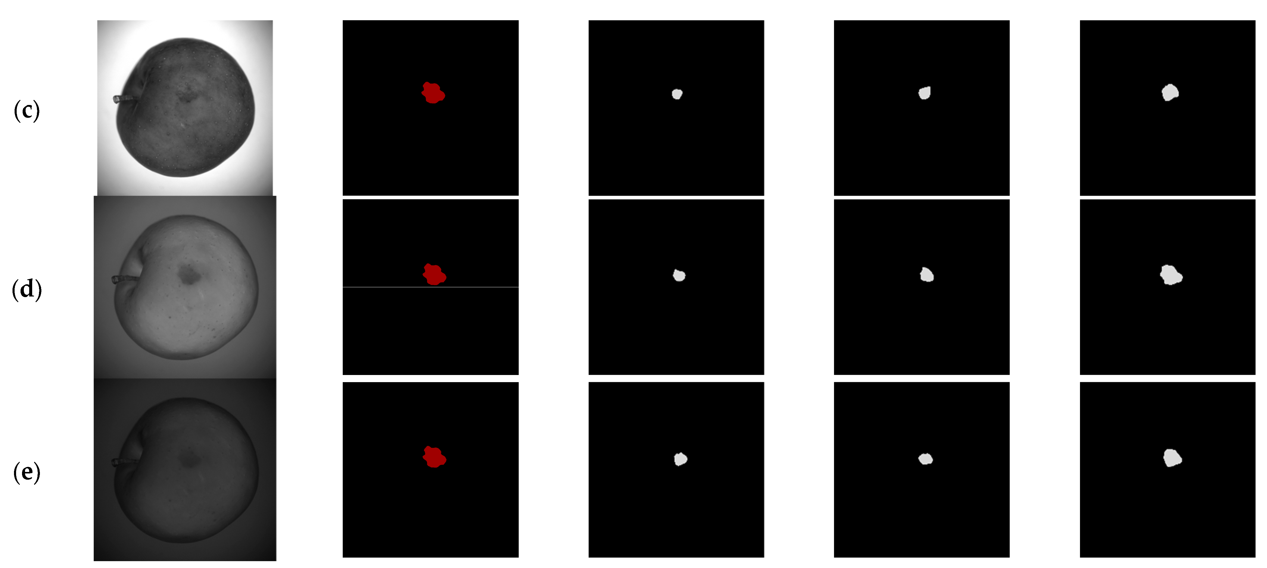
The traditional algorithm shown in Figure 5, the trained U-Net, and the trained improved U-Net were used to extract defects of apples in the test set, and the results of manual extraction were used as a comparison. The specific extraction results are shown in Figure 13 and Figure 14.

At 460 and 660 nm, the characteristics of the defective areas on the apple surface were similar to those of the normal areas. At 522 nm, the textural characteristics of the apple surface were similar to the defective characteristics. At 762 and 842 nm in the near-infrared band, the defects became clear and the textural features of the apple were weakened. Therefore, when the defects of the five single-band images were extracted by using the same algorithm, the single-band image at 762 nm performed best.

Under the same band, when the traditional algorithms were used to extract defects, there were incomplete segmentation and mis-segmentation. The U-Net extracts image features through multiple convolutional layers, then by learning from a large number of samples, higher accuracy is achieved. Compared with the traditional algorithm, this situation was improved. However, due to the imbalance between the positive sample and the negative sample, when the U-Net was used to extract such defect, incomplete segmentation and mis-segmentation still existed. By using dilated convolution, adding attention gates to the original U-Net, and during the training process, using the weighted binary cross-entropy loss function, the improved U-Net paid more attention to the defective area. Compared with the traditional algorithm and the original U-Net, the improved U-Net could extract more complete defects.

For defects with small areas and irregular edges, incomplete segmentation occurred by using the traditional algorithms. Additionally, the U-Net only segmented the outline of the defects, and the segmentation of the defective edges was still rough. In this study, during the training process, the improved U-Net used a boundary loss function that made the network start paying attention to the segmentation of defective edges. Therefore, compared with the traditional algorithm and the original U-Net, the improved U-Net was more detailed for the segmentation of the defective edges.

3.3. Analysis of Indicators

The mIoU and mF1-score of the traditional algorithm, the U-Net, and the improved U-Net on the test set are shown in

Table 2. mIoU of the traditional algorithm, U-Net, and improved U-Net.

	460 nm	522 nm	660 nm	762 nm	842 nm	Average
Traditional Algorithm	0.62	0.66	0.68	0.73	0.70	0.68
U-Net	0.72	0.74	0.78	0.82	0.79	0.77
The Improved U-Net	0.81	0.83	0.85	0.91	0.87	0.85
Average	0.72	0.74	0.77	0.82	0.79	None

and

Table 3. mF1-score of the traditional algorithm, U-Net, and improved U-Net.

	460 nm	522 nm	660 nm	762 nm	842 nm	Average
Traditional Algorithm	0.74	0.78	0.81	0.84	0.81	0.80
U-Net	0.83	0.86	0.87	0.89	0.88	0.87
The Improved U-Net	0.88	0.90	0.91	0.95	0.92	0.91
Average	0.82	0.85	0.86	0.89	0.87	None

, respectively.

When segmenting apple surface defects by using the same algorithm, the mIoU and the mF1-score in the visible range are lower than those in the near-infrared range. More specially, at 460 nm, the mIoU and mF1-score are the lowest, with averages of 0.72 and 0.82. At 762 nm, the mIoU and mF1-score are the highest, with averages of 0.82 and 0.89.

Under the same band, the mIoU and mF1-score of the U-Net are higher than those of the traditional algorithm. Based on the U-Net, the indicators of the improved U-Net are further improved. Therefore, the traditional algorithm has the lowest mIoU and mF1-score with averages of 0.68 and 0.80. The improved U-Net has the highest mIoU and mF1-score with averages of 0.85 and 0.91.

Combining band and segmentation algorithms, the highest mIoU and mF1-score are obtained at 762 nm by using the improved U-Net, 0.91 and 0.95, respectively.

4. Conclusions

For defects with unobvious features, small areas, and irregular edges, defect extraction was not effective by using the traditional algorithm in the visible range. There were incomplete segmentation, mis-segmentation, and so on. In this study, with the help of multi-band images and a modified convolutional neural network, when such defects were extracted, the accuracy was increased. The experimental results show that in the visible range, the traditional algorithm performed worst at 460 nm with an mIoU of 0.62 and an mF1-score of 0.74; in the near-infrared range, the improved U-Net performed best at 762 nm with an mIoU of 0.91 and an mF1-score of 0.95.