1. Introduction
Squash (
Cucurbita pepo L.) is a popular cucurbit vegetable crop in many parts of the world. It is a commercial crop that is grown in both open fields and greenhouses, particularly in the Mediterranean region [
1,
2,
3]. It provides numerous medicinal and health benefits for humans [
4], as well as adequate levels of proteins, minerals, vitamins and carbohydrates for human nutrition [
5].
Water scarcity is regarded as the most significant constraint to plant growth and development in arid and semi-arid environments, yielding more than any other environmental factors [
6,
7,
8,
9,
10]. It is clear that a lack of water, even for a short period, alters the physio-biochemical characteristics of crops, which inhibits their growth and productivity [
11,
12,
13].
Fertilization is also important for absorbing macronutrients, determining their amount in various plant organs, and determining final yield. Due to the quick accumulation of vegetable mass in a relatively short period of harvest, squash crops are fertilization-responsive vegetable crops [
14,
15,
16]. Potassium is a vital nutrient for plant growth and development, so developing an optimal water–potassium fertilization management strategy to improve their application efficiency is crucial [
17,
18].
In locations where there is a lack of moisture and fertilization, agricultural crop production is always monitored using point-sampling techniques (traditional methods), which are laborious, expensive, and seem to have poor spatial representation [
19,
20,
21,
22,
23]. Therefore, to support current agricultural practices, especially in nations where current agricultural systems are unable to meet the high demands of rapid population growth, robust and fast techniques for spotting stress in various agricultural crops are necessary. Accurate, rapid, non-destructive, and cost-effective estimation of a wide range of phenotypic crop traits is possible with the help of proximal remote sensing, which can complement or even replace traditional methods [
24,
25,
26]. The remote sensing technique can detect even minor changes in various biophysical and biochemical aspects of the plant canopy caused by moisture and or fertilization deficiencies in the range from the visible (VIS) to the near-infrared (NIR) and shortwave infrared (SWIR). Broadly, changes in above-ground biomass, leaf pigments, leaf area index, leaf water content and nutrient content are reflected in changes in the crop canopy’s spectral signature [
27,
28]. Plant pigments, such as chlorophyll and carotenoids, absorb a lot of visible light, especially blue and red light. Furthermore, the diffusion and scattering of radiation as a result of dry matter and leaf tissues has a significant impact on canopy reflectance in the NIR range [
29,
30,
31,
32,
33].
Spectral vegetation indices derived from in situ ground-based remotely sensed data have been shown in prior studies to be useful for identifying stressed vegetation in a wide range of agricultural crops. These include, for example: the determination of aerial plant biomass [
34,
35,
36,
37]; chlorophyll a concentration [
38,
39,
40,
41,
42]; crop grain yield [
43,
44]; leaf area index [
45,
46,
47]; nitrogen content [
48,
49]; water stress [
31,
50]; pest injuries; and plant diseases [
25,
51,
52]. Many earlier research studies have shown that ground-based remotely sensed data can be utilized to evaluate growth parameters and crop health status; however, most of the studies concentrated on detecting moisture shortage stress, whereas potassium deficiency has received comparatively less attention in the literature. This study examined the feasibility of utilizing ground-based remote sensing to detect potassium and moisture stress at the canopy scale. It is crucial to make measurements at the canopy scale in order to evaluate how well satellite imagery might be used for site-specific management.
Model-based feature selection methods, for example, identify a subset of features with strong discriminative and foretelling power [
53]. By reducing extraneous features and limiting over-fitting, this method can improve model performance. Moreover, it retains the initial feature representation, which boosts interpretability [
54]. Prediction and modeling increasingly require feature selection algorithms [
55]. Many research studies have been conducted to investigate the use of various strategies for dimensionality reduction in data. Each variable’s weighed regression coefficient in the partial least-squares (PLS) model highlights the importance of wavelength in the model for partial least-square regression (PLSR) [
56]. In the decision tree (DT) and random forest (RF), all variables are ranked in order of relevance [
57]. Glorfeld [
58] created a back-propagation neural network index for identifying the most important variables. Furthermore, hyper-parameter selection has a substantial influence on the ability of any machine learning (ML) model, which has numerous benefits: it has the potential to improve the performance of ML algorithms [
59], as well as the repeatability and fairness of scientific studies [
60]. It might play a crucial role in improving the prediction model because it has direct influence over training algorithm behavior [
61]. Consequently, we may expect that changing hyper-parameters will have a remarkable influence on the accuracy of squash crop quality measurements.
The objectives of the current study were to (i) estimate the effects of irrigation treatments and potassium fertilization on four traits of squash (KUE, Chlm, WUE and SY); (ii) evaluate the performance of common and three-band SRIs to assess the four traits of squash; (iii) assess the potential role of ground-based remote sensing based on spectral bands to detect and distinguish water and potassium stress spectrally; and (iv) evaluate the performance of the DT model based on the spectral bands, SRIs and data fusion of both spectral bands, and of SRIs to predict the four investigated traits of squash.
2. Materials and Methods
2.1. Experimental Description
Over the spring and fall seasons of 2018, two field experiments were conducted at a private farm in the Elshagaa region, Egypt (latitude of 30°4′12″ N and longitude of 30°19′48″ E). Non-disturbed soil samples were taken at two depths of the soil profile (0–30, and 30–60 cm) to identify some physical and chemical characteristics of the experimental soil, which was classified as loamy sand in texture, with an average bulk density of 1.53 g cm
−3, an electrical conductivity (EC) of 1.32 dS m
−1, and a pH of 7.39. The particle size distribution was found to be 87.3% sand, 6.36% silt, and 6.34% clay. The chemical analysis of the experimental soil, which includes cations and anions, is shown in
Table 1. Squash was planted in the first week of March and the last week of July, with a growing season of around 100 days from planting to harvest. In addition, the soil’s hydrophysical characteristics were determined as detailed in
Table 2. Nitrogen fertilization in the form of ammonium nitrate was applied in three equal doses at 30, 45 and 60 days after planting at a rate of 285 kg N ha
−1.
2.2. Solar–Powered Pumping and Drip Irrigation Systems
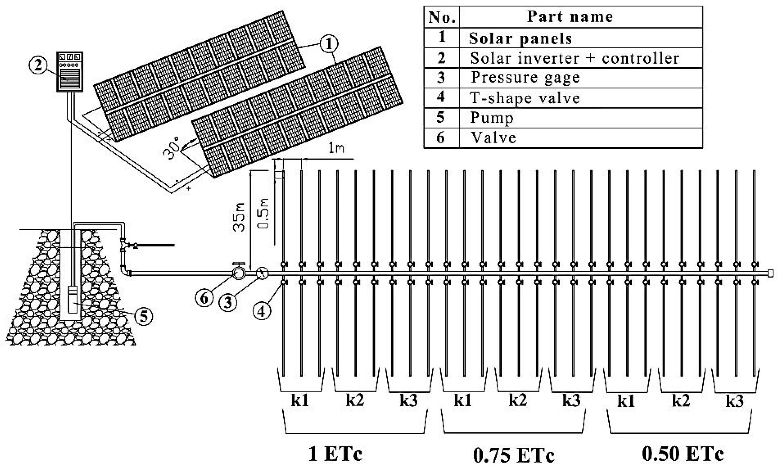
The solar–powered pumping system comprised 40 solar cells (JKM 250P-60) placed in two groups of 20 modules each, which were connected in series before being connected together in parallel (
Figure 1). Every solar module measured 165 cm length, 99.2 cm in width and 4 cm in thickness. To collect the most sunlight, the solar cell system was directed toward the south. The 40 PV cells (250 W) generated enough energy required to operate the submersible pump, which supplied the required amount of water for the entire farm. This solar-powered irrigation system was built to irrigate around 10 hectares farm. Solar radiation fluctuated throughout the year, with maximum and minimum values of 7.1 and 3.8 kWh m
−2 recorded in June and December, respectively. The solar power system was connected to a 10 kW power controller (PS9K2) with 98% overall efficiency. Water was delivered to either a drip irrigation system or a concrete water reservoir (10 m length × 10 m width × 5 m depth) by a 7.5 kW PUC-SJ30-7 submersible pump.
The drip irrigation system was used to irrigate the experimental plots, which consisted of 16 mm polyethylene lateral lines spaced at 1.0 m and emitters spaced at 0.5 m. In the system, a pressure differential tank was installed for the application of different fertilizers. An experimental unit was tested with three replicates using a split-plot design with nine 35 m long lateral lines with 4 L h−1 built-in emitters. The primary plots received irrigation treatments at random, while the secondary plots received K rates. Using Class A pan evaporation data, the applied irrigation water was determined based on reference evapotranspiration (ETo). With three replicates, the experiment was set as a split-plot design. The primary plots were watered at a certain pace, whereas the secondary plots were fertilized with potassium at a different rate. Squash plants were given nine various combinations of moisture (1.00, 0.75 and 0.50 ETc) and potassium rates (100, 150 and 250 kg K ha−1). Starting two weeks after planting, potassium fertilization was applied weekly throughout the growing cycle, with the total amount of K varying based on the rate of each treatment. All experimental plots were fully irrigated for 21 days to guarantee the best germination ratio, and then various treatments were applied.
2.3. Calculation of Irrigation Water Requirements
According to the formula of Doorenbos and Kassam [
62], reference evapotranspiration (
ETo) was calculated according to the Class A pan evaporation technique as follows:
where
ETo represents the reference evapotranspiration (mm d
−1),
Epan represents the daily measured pan evaporation (mm d
−1), and
Kpan is the pan coefficient, which was taken as 0.75 for the experimental location based on the local climatic conditions. According to Vermeiren and Jopling [
63], the total irrigation water applied was calculated as follows:
where
AIW represents the total depth of applied water, mm;
ETo the reference evapotranspiration, mm day
−1; and the reduction factor,
Kr, is influenced by the type of ground cover. According to James [
64], this was assumed to be 1.0 (spacing between drip lines was <1.8 m).
Ea is the drip irrigation system efficiency, which was assumed to be on average 0.8. I is the irrigation interval, days.
Irrigation time was identified before each irrigation event according to Ismail [
65] as follows:
where
T is the duration of irrigation (h),
A is the area sprayed by each emitter (m
2), and
q is the discharge rate of the emitters (h
−1 L).
According to the previous equations, the total amounts of water applied to different treatments in both investigated seasons were 371 and 308 mm for 1.00 ETc for the spring and fall seasons, respectively. The watering regimes of 0.75 and 0.50 ETc were then identified as percentages of 1.00 ETc for both seasons.
2.4. Determination of Squash Seed Yield and Chlorophyll Meter
At harvest, a 4 m2 area from each treatment was collected to assess the overall production of squash seeds. Concurrent with collecting spectra reflectance from the squash canopy, we also measured the Chlm at the leaves. Each treatment’s Chlm was measured with the use of a handheld SPAD chlorophyll meter (Konica-Minolta, Osaka, Japan).
2.5. Water-Use Efficiency
The following equation was implemented to determine water-use efficiency:
2.6. Potassium-Use Efficiency (KUE)
Potassium-use efficiency represents the ratio between squash seed yield and the entire amount of potassium added to the crop over the growing season, and was calculated as follows:
where
KUE represents the potassium-use efficiency, kg of squash seeds (kg K
2O
5)
−1;
Y refers to the seed squash yield in kg ha
−1 in a certain treatment; and
K is the applied amount of K
2O
5 to the same treatment.
2.7. Reflectance Measurement Acquisition and Selection of Spectral Reflectance Indices
The spectra of squash plants’ canopies were measured with a spectroradiometer from ASD that had a field of view of 3.5°. Because of the need for a wider scanning area, the detector was mounted on the end of a telescopic pole and maintained at a fixed height of about 1.25 m above the ground. The spectrometer could measure light with a wavelength of from 350 nm to 1075 nm. On cloud-free days between 11:30 to 13:30 h GMT, spectra were acquired from crop canopies under sun radiation. The spectrum reflectance of the sensor was calibrated using a white spectralon. Processed spectra were then used to derive different SRI
s.
Table 3 lists some of the most widely used SRI
s as well as the method for calculating, along with references. Eighteen SRIs, including the six most widely used SRI
s and twelve freshly advanced three-band (3-D) SRIs, were examined (
Table 3). Statistics were displayed on contour maps as determination coefficients (R
2) between four measured parameters (KUE, Chlm, WUE, and SY) with three-band SRIs (
Figure 2). These indices were calculated by integrating potentials at any three wavelengths from a spectrum region ranging from 390 to 750 nm. According to Elsayed et al. [
66], three-dimensional spectral reflectance maps were created. The provided maps are critical for establishing the optimal spectral region with feasible wavelengths and understanding the significance of three-band SRIs (
Table 3).
2.8. Decision Tree (DT)
Decision tree induction is the process of training decision trees using class-labelled training tuples. A decision tree is a tree structure like a flowchart. The DT algorithm is composed of several nodes, each of which has a root, a leaf, and a decision. The root node is the one that starts the tree, and the decision nodes are the ones that are responsible for deciding what to do next, which means going from one node to another. The decision nodes are responsible for producing the leaf nodes. While some decision tree algorithms are limited to producing binary trees (having only two internal nodes), others are able to produce more complex trees [
72]. As a result of their frequent usage in research [
73], maximum depth (Md), maximum leaf nodes (Mln), and minimum sample leaf (S) were taken into consideration during training. For Md, Ms, and Mln, the parameter values were (1, 3, 5, 7), (2, 4, 6, 8), and (none, 10, 20, 30), respectively. By concentrating on these hyperparameters, we adjusted the model. In general, the model was supplied with the various characteristics at random during the first iteration, the low-level parameters were eliminated after each iteration, and the excellent parameters were retained with regard to the highest contribution. Then, all model outcomes were evaluated to choose high-quality parameters with a low model loss to accurately assess squash properties under moisture- and potassium-deficit stress. The DT can be easily transformed into regression rules. Because it does not need domain expertise or parameter setting, building decision tree regressors is ideal for exploratory knowledge discovery. The DTs used in this model are capable of handling high-dimensional input with accuracy. The DT models were based on spectral bands, SRIs and data fusion of both spectral bands, and SRIs were used to predict the four investigated traits (KUE, Chlm, WUE and SY) of squash.
2.9. Datasets and Software for Data Analysis
About 54 samples were utilized for training and validation; of these, 41 samples (or 80%) were used to exercise and test the regression model. However, the remaining 10 instances (or 20%) were employed to gauge the model’s performance by contrasting projected and measured values. Before training, to correct for size disparities across various features, normalization was converted across individual features. By removing the minimal spectral data and dividing the difference between the highest and lowest feature values, feature normalization was calculated. Then, the model was trained and validated using a leave-one-out cross-validation (LOOCV) method. In each trial, LOOCV utilized the remaining data for training while excluding one sample for validation. This approach can lessen over-fitting and provide a more precise evaluation of the model’s predictive power [
73]. Data analysis, model construction, and data preparation were all carried out using Python 3.7.3 software. Research was conducted on the DT module, which is a part of the Scikit-learn package, version 0.20.2. This was carried out in order to finish the regression tasks. The examination of the data was carried out on a machine with an Intel Core i7–3630QM processor running at 2.4 GHz and 8 gigabytes of RAM.
2.10. Model Evaluation
The root mean square error (RMSE) and the coefficient of determination (R
2) are two statistical metrics that are applied in order to evaluate the efficacy of a regression model [
74,
75]. All the parameters that are being described are as follows: the term “
Fact” refers to the actual value that was computed in the laboratory; “
Fp” stands for the value that was predicted or simulated; “
N” represents for the total number of data points; and “
Fave” indicates the value that was averaged out over all the data points.
Coefficient of determination:
2.11. Statistical Analysis
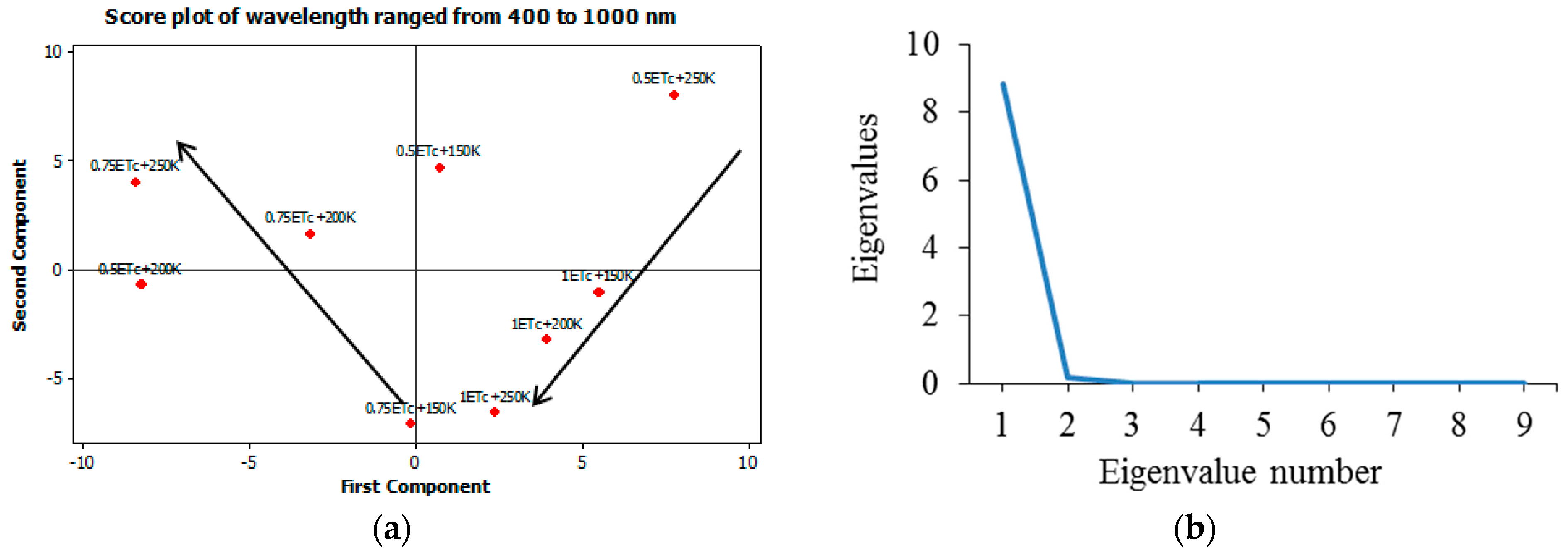
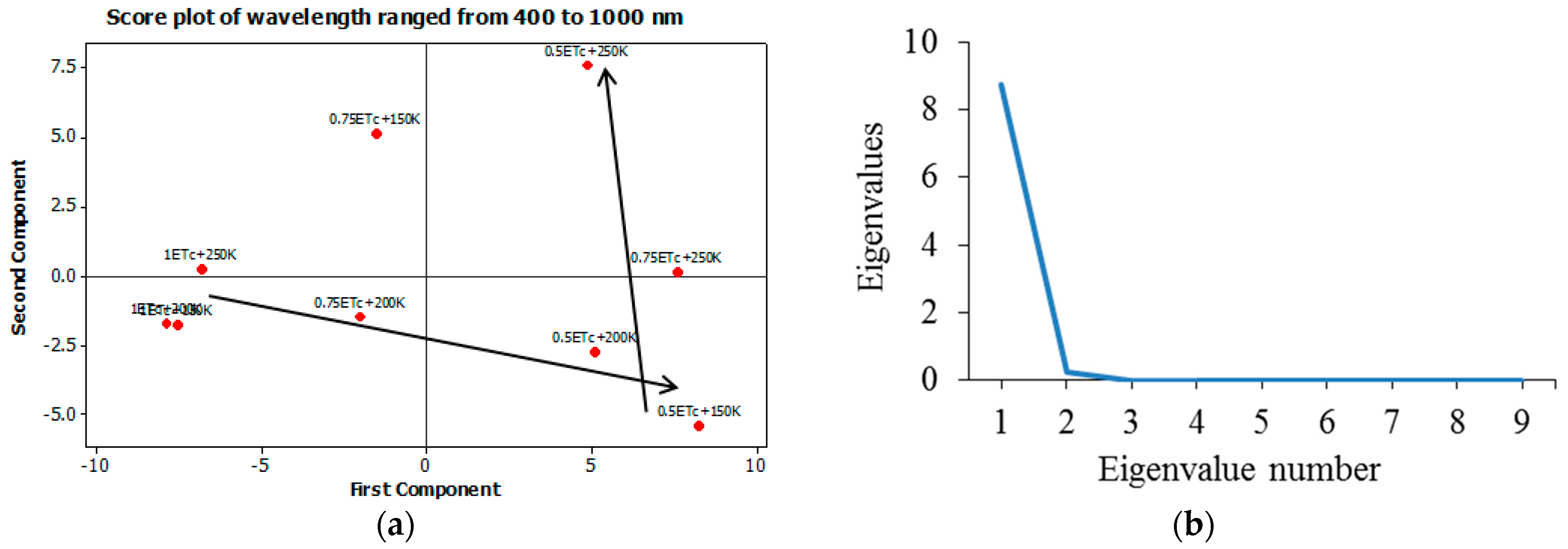
Combined analysis of variance across the two seasons was performed after performing the homogeneity test. The analysis of variance (ANOVA) of the split plot design was performed with irrigation regime (I) as the main-plot treatment in three levels, and potassium fertilizer (K) as a subplot factor in three rates, with three replicates for each level. Statistical analysis included analysis of variance (degrees of freedom (df), F-values, and significance level) of the effect of year, irrigation level, potassium level, and their interaction on SY, Chlm, WUE, KUE and spectral indices of squash. Least-significant differences (LSD) values were calculated to test the significance of differences between means. The Duncan test was performed to examine the significant difference of measured characteristics and SRIs of squash under varied nitrogen levels. Mean values with the same letter did not differ significantly (p ≤ 0.05). Simple regressions were used to calculate the association between the SRIs and the assessed attributes. The 0.05, 0.01 and 0.001 probability levels were used to establish the significance level of the coefficients of determination (R2) for these relationships. Using the collected spectra, which comprised all wavelengths from all treatments, principal component analysis (PCA) was used to assess differences and distinguish the spectral responses of non-stressed and stressed squash plants. The spectra collected from each plot were averaged, and the overall mean spectrum was examined in PCA to initially observe differences in the spectral signature acquired from healthy and varying stressed treatments (moisture and potassium deficiency). The raw data for the nine different treatments were composed of 135 columns and more than a thousand rows; therefore, we averaged the data to compress it, given the large size of the raw data. The different statistical analysis and plotting were performed using SPSS 22 (SPSS Inc., Chicago, IL, USA) and Minitab v.14 (Minitab Inc., State college, PA, USA).
4. Conclusions
This investigation tested the potential of spectral reflectance measurements to determine squash properties and find dissimilarities between non-stressed and stressed squash plants. Few studies of this kind have produced three-dimensional contour maps employing SRIs to evaluate these characteristics across varying water regimes and potassium fertilizer rates. The results demonstrated the sensitivity of the newly constructed three-band SRIs for estimating the four squash parameters, with wavelengths spanning the visible (VIS), red-edge, and near-infrared (NIR) domains. The results showed that the newly built three-band SRIs, covering the visible (VIS), red-edge (RE), and near-infrared (NIR) spectral ranges, were sensitive enough to estimate the four tested squash parameters. The results further demonstrated that the PCA showed the ability to separate moisture induced stress from potassium deficiency stress at the flowering stage onwards. The DT model’s prediction accuracy is affected by the value and number of features. The results of the models shows a variety of choices for merging features and models that have the greatest influence on the prediction of quality attributes in squash crops. The DT-SRIs-1 model scored better at forecasting SY than the others. The model’s R2 performance for the training and validation datasets, respectively, was 0.799 (RMSE = 97.473) and 0.699 (RMSE = 87.656). The overall results demonstrate that proximal reflectance sensing based on SRIs, as well as a DT model including spectral bands, SRIs or their combinations, could be used to estimate the four squash parameters under different levels of water regimes and potassium fertilization rates.


 ,
, 


