
Fast Calculations for the Magnetohydrodynamic Flow and Heat Transfer of Bingham Fluids with the Hall Effect


Abstract
1. Introduction
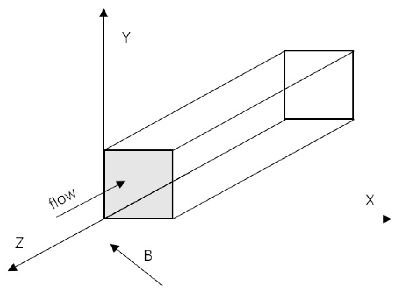
2. Mathematical Model
3. Numerical Method
3.1. Direct Method
3.2. Fast Method
4. Numerical Examples
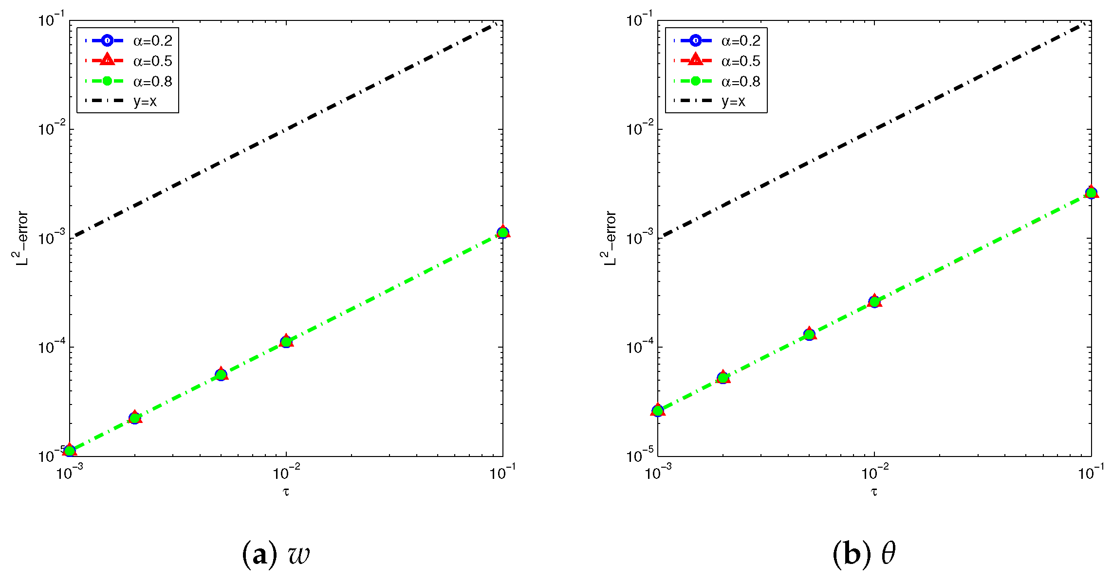
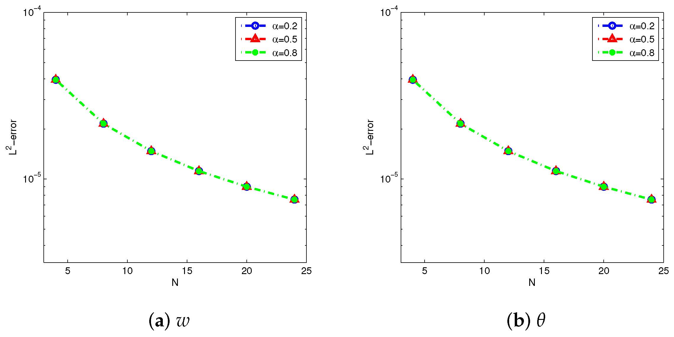
4.1. Example 1
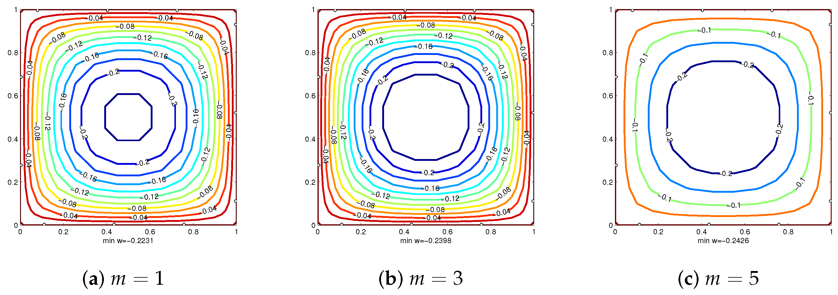
4.2. Example 2
5. Conclusions
Author Contributions
Funding
Data Availability Statement
Conflicts of Interest
References
- Dehghan, M.; Abbaszadeh, M. Analysis of the element free Galerkin (EFG) method for solving fractional cable equation with Dirichlet boundary condition. Appl. Numer. Math. 2016, 109, 208–234. [Google Scholar] [CrossRef]
- Wang, X.; Xu, H.; Qi, H. Transient magnetohydrodynamic flow and heat transfer of fractional Oldroyd-B fluids in a microchannel with slip boundary condition. Phys. Fluids 2020, 32, 103104. [Google Scholar] [CrossRef]
- Liu, Y.; Zhang, H.; Jiang, X. Fast evaluation for magnetohydrodynamic flow and heat transfer of fractional Oldroyd-B fluids between parallel plates. ZAMM-J. Appl. Math. Mech./Z. Angew. Math. Mech. 2021, 101, e202100042. [Google Scholar] [CrossRef]
- Jiang, Y.; Sun, H.; Bai, Y.; Zhang, Y. MHD flow, radiation heat and mass transfer of fractional Burgers’ fluid in porous medium with chemical reaction. Comput. Math. Appl. 2022, 115, 68–79. [Google Scholar] [CrossRef]
- Vishalakshi, A.B.; Mahesh, R.; Mahabaleshwar, U.S.; Rao, A.K.; Pérez, L.M.; Laroze, D. MHD hybrid nanofluid flow over a stretching/shrinking sheet with skin friction: Effects of radiation and mass transpiration. Magnetochemistry 2023, 9, 118. [Google Scholar] [CrossRef]
- Shahid, N. A study of heat and mass transfer in a fractional MHD flow over an infinite oscillating plate. SpringerPlus 2015, 4, 640. [Google Scholar] [CrossRef]
- Zhang, Y.; Jiang, J.; Bai, Y. MHD flow and heat transfer analysis of fractional Oldroyd-B nanofluid between two coaxial cylinders. Comput. Math. Appl. 2019, 78, 3408–3421. [Google Scholar] [CrossRef]
- Qiao, Y.; Wang, X.; Xu, H.; Qi, H. Numerical analysis for viscoelastic fluid flow with distributed/variable order time fractional Maxwell constitutive models. Appl. Math. Mech. 2021, 42, 1771–1786. [Google Scholar] [CrossRef]
- Osalusi, E.; Side, J.C.; Harris, R.E.; Johnston, B. On the effectiveness of viscous dissipation and Joule heating on steady MHD and slip flow of a Bingham fluid over a porous rotating disk in the presence of Hall and ion-slip currents. JP J. Heat Mass Transf. 2007, 1, 303–330. [Google Scholar] [CrossRef]
- Rathod, V.P.; Laxmi, D.V. Effects of heat transfer on the peristaltic MHD flow of a Bingham fluid through a porous medium in a channel. Int. J. Biomath. 2014, 7, 1450060. [Google Scholar] [CrossRef]
- Povstenko, Y.; Kyrylych, T. Time-Fractional Heat Conduction in a Plane with Two External Half-Infinite Line Slits under Heat Flux Loading. Symmetry 2019, 11, 689. [Google Scholar] [CrossRef]
- Liu, Y.; Chi, X.; Xu, H.; Jiang, X. Fast method and convergence analysis for the magnetohydrodynamic flow and heat transfer of fractional Maxwell fluid. Appl. Math. Comput. 2022, 430, 127255. [Google Scholar] [CrossRef]
- Zhang, H.; Liu, F.; Phanikumar, M.S.; Meerschaert, M.M. A novel numerical method for the time variable fractional order mobile-immobile advection-dispersion model. Comput. Math. Appl. 2013, 66, 693–701. [Google Scholar] [CrossRef]
- Zeng, F.; Liu, F.; Li, C.; Burrage, K.; Turner, I.W.; Anh, V.V. A Crank-Nicolson ADI Spectral Method for a Two-Dimensional Riesz Space Fractional Nonlinear Reaction-Diffusion Equation. SIAM J. Numer. Anal. 2014, 52, 2599–2622. [Google Scholar] [CrossRef]
- Ji, C.; Dai, W.; Sun, Z. Numerical Method for Solving the Time-Fractional Dual-Phase-Lagging Heat Conduction Equation with the Temperature-Jump Boundary Condition. J. Sci. Comput. 2018, 75, 1307–1336. [Google Scholar] [CrossRef]
- Jajarmi, A.; Ghanbari, B.; Baleanu, D. A new and efficient numerical method for the fractional modeling and optimal control of diabetes and tuberculosis co-existence. Chaos 2019, 29, 093111. [Google Scholar] [CrossRef]
- Kumar, S.; Ahmadian, A.; Kumar, R.; Kumar, D.; Singh, J.; Baleanu, D.; Salimi, M. An Efficient Numerical Method for Fractional SIR Epidemic Model of Infectious Disease by Using Bernstein Wavelets. Mathematics 2020, 8, 558. [Google Scholar] [CrossRef]
- Yang, S.; Liu, F.; Feng, L.; Turner, I.W. Efficient numerical methods for the nonlinear two-sided space-fractional diffusion equation with variable coefficients. Appl. Numer. Math. 2020, 157, 55–68. [Google Scholar] [CrossRef]
- Liu, F.; Turner, I.W.; Anh, V.V.; Yang, Q.; Burrage, K. A numerical method for the fractional Fitzhugh–CNagumo monodomain model. Sci. Eng. Fac. 2013, 54, C608–C629. [Google Scholar]
- Yu, B.; Jiang, X.; Qi, H. Numerical method for the estimation of the fractional parameters in the fractional mobile/immobile advection–Cdiffusion model. Int. J. Comput. Math. 2018, 95, 1131–1150. [Google Scholar] [CrossRef]
- Zheng, R.; Zhang, H.; Jiang, X. Legendre spectral methods based on two families of novel second-order numerical formulas for the fractional activator-inhibitor system. Appl. Numer. Math. 2021, 162, 235–248. [Google Scholar] [CrossRef]
- Huang, Y.; Zeng, F.; Guo, L. Error estimate of the fast L1 method for time-fractional subdiffusion equations. Appl. Math. Lett. 2022, 133, 108288. [Google Scholar] [CrossRef]
- Farquhar, M.E.; Moroney, T.J.; Yang, Q.; Turner, I.W. GPU accelerated algorithms for computing matrix function vector products with applications to exponential integrators and fractional diffusion. SIAM J. Sci. Comput. 2016, 38, C127–C149. [Google Scholar] [CrossRef]
- Krishnarjuna, B.; Chandra, K.; Atreya, H.S. Accelerating NMR-Based Structural Studies of Proteins by Combining Amino Acid Selective Unlabeling and Fast NMR Methods. Magnetochemistry 2017, 4, 2. [Google Scholar] [CrossRef]
- Jia, J.; Zheng, X.; Wang, H. A fast method for variable-order space-fractional diffusion equations. Numer. Algorithms 2019, 85, 1519–1540. [Google Scholar] [CrossRef]
- Fang, Z.; Sun, H.; Wang, H. A fast method for variable-order Caputo fractional derivative with applications to time-fractional diffusion equations. Comput. Math. Appl. 2020, 80, 1443–1458. [Google Scholar] [CrossRef]
- Cao, J.; Xiao, A.; Bu, W. Finite Difference/Finite Element Method for Tempered Time Fractional Advection–Dispersion Equation with Fast Evaluation of Caputo Derivative. J. Sci. Comput. 2020, 83, 1–29. [Google Scholar] [CrossRef]
- Wang, P. Fast exponential time differencing/spectral-Galerkin method for the nonlinear fractional Ginzburg-Landau equation with fractional Laplacian in unbounded domain. Appl. Math. Lett. 2021, 112, 106710. [Google Scholar] [CrossRef]
- Zhu, H.; Xu, C. A Fast High Order Method for the Time-Fractional Diffusion Equation. SIAM J. Numer. Anal. 2019, 57, 2829–2849. [Google Scholar] [CrossRef]
- Alikhanov, A.A. A new difference scheme for the time fractional diffusion equation. J. Comput. Phys. 2015, 280, 424–438. [Google Scholar] [CrossRef]
- Jia, J.; Wang, H.; Zheng, X. Numerical Analysis of a Fast Finite Element Method for a Hidden-Memory Variable-Order Time-Fractional Diffusion Equation. J. Sci. Comput. 2022, 91, 54. [Google Scholar] [CrossRef]
- Chi, X.; Zhang, H.; Jiang, X. The fast method and convergence analysis of the fractional magnetohydrodynamic coupled flow and heat transfer model for the generalized second-grade fluid. Sci. China Math. 2023, 67, 919–950. [Google Scholar] [CrossRef]
- Jiang, S.; Zhang, J.; Zhang, Q.; Zhang, Z. Fast evaluation of the Caputo fractional derivative and its applications to fractional diffusion equations. Commun. Comput. Phys. 2017, 21, 650–678. [Google Scholar] [CrossRef]
- Xiao, J.; Chen, Y.; Zeng, F.; Zhang, Z. L1 Schemes for time-fractional differential equations: A brief survey and new development. Res. Sq. 2024. posted. [Google Scholar]
- Zhao, J.; Zheng, L.; Zhang, X.; Liu, F. Convection heat and mass transfer of fractional MHD Maxwell fluid in a porous medium with Soret and Dufour effects. Int. J. Heat Mass Transf. 2016, 103, 203–210. [Google Scholar] [CrossRef]
- Cowling, T. Magnetohydrodynaics; Interscience: New York, NY, USA, 1957. [Google Scholar]
- Liu, Y.; Guo, B. Coupling model for unsteady MHD flow of generalized Maxwell fluid with radiation thermal transform. Appl. Math. Mech. 2016, 37, 137–150. [Google Scholar] [CrossRef]
- Podlubny, I. Fractional Differential Equations; Academic Press: New York, NY, USA, 1999. [Google Scholar]
- Sun, Z.; Wu, X. A fully discrete difference scheme for a diffusion-wave system. Appl. Numer. Math. 2006, 56, 193–209. [Google Scholar] [CrossRef]
- Liu, L.; Yang, S.; Feng, L.; Xu, Q.; Zheng, L.; Liu, F. Memory dependent anomalous diffusion in comb structure under distributed order time fractional dual-phase-lag model. Int. J. Biomath. 2021, 14, 2150048. [Google Scholar] [CrossRef]
- Shen, J.; Tang, T.; Wang, L. Spectral Methods: Algorithms, Analysis and Applications; Springer: Berlin/Heidelberg, Germany, 2011. [Google Scholar]


| w | ||||
|---|---|---|---|---|
| Error | Rate | Error | Rate | |
| 1/10 | 1.1254 | - | 2.6136 | - |
| 1/100 | 1.1181 | 1.0028 | 2.6110 | 1.0004 |
| 1/200 | 5.5873 | 1.0008 | 1.3051 | 1.0004 |
| 1/500 | 2.2352 | 0.9986 | 5.2191 | 1.0003 |
| 1/1000 | 1.1174 | 1.0003 | 2.6090 | 1.0003 |
Disclaimer/Publisher’s Note: The statements, opinions and data contained in all publications are solely those of the individual author(s) and contributor(s) and not of MDPI and/or the editor(s). MDPI and/or the editor(s) disclaim responsibility for any injury to people or property resulting from any ideas, methods, instructions or products referred to in the content. |
© 2025 by the authors. Licensee MDPI, Basel, Switzerland. This article is an open access article distributed under the terms and conditions of the Creative Commons Attribution (CC BY) license (https://creativecommons.org/licenses/by/4.0/).
Share and Cite
Tian, Y.; Liu, Y. Fast Calculations for the Magnetohydrodynamic Flow and Heat Transfer of Bingham Fluids with the Hall Effect. Magnetochemistry 2025, 11, 21. https://doi.org/10.3390/magnetochemistry11030021
Tian Y, Liu Y. Fast Calculations for the Magnetohydrodynamic Flow and Heat Transfer of Bingham Fluids with the Hall Effect. Magnetochemistry. 2025; 11(3):21. https://doi.org/10.3390/magnetochemistry11030021
Chicago/Turabian StyleTian, Ye, and Yi Liu. 2025. "Fast Calculations for the Magnetohydrodynamic Flow and Heat Transfer of Bingham Fluids with the Hall Effect" Magnetochemistry 11, no. 3: 21. https://doi.org/10.3390/magnetochemistry11030021
APA StyleTian, Y., & Liu, Y. (2025). Fast Calculations for the Magnetohydrodynamic Flow and Heat Transfer of Bingham Fluids with the Hall Effect. Magnetochemistry, 11(3), 21. https://doi.org/10.3390/magnetochemistry11030021