Cross-Stitch Networks for Joint State of Charge and State of Health Online Estimation of Lithium-Ion Batteries

Abstract

As a superior solution to the developing demand for energy storage, lithium-ion batteries play an important role in our daily lives. To ensure their safe and efficient usage, battery management systems (BMSs) are often integrated into the battery systems. Among other critical functionalities, BMSs provide information about the key states of the batteries under usage, including state of charge (SOC) and state of health (SOH). This paper proposes a data-driven approach for the joint online estimation of SOC and SOH utilizing multi-task learning (MTL) approaches, particularly highlighting cross-stitch units and cross-stitch networks. The proposed model is able to achieve an accurate estimation of SOC and SOH in online applications with optimized information sharing and multi-scale implementation. Comprehensive results on training and testing of the model are presented. Possible improvements for future work are also discussed in the paper.

1. Introduction

As public awareness about environmental protection grows, society has pivoted its attention to technologies and applications of clean, renewable energy. This shift in focus has greatly accelerated the development of energy storage technologies, which are essential for the storage and exploitation of renewable energy sources, e.g., solar and wind. Among the rapidly evolving landscape of energy storage technologies, lithium-ion batteries have stood out with their high energy density and high power density [1]. These characteristics have made them ideal for powering diverse applications ranging from portable electronics [2] to electric vehicles [3], power grid systems, and even aerospace applications. To ensure the safe and efficient usage of lithium-ion batteries, a so-called battery management system (BMS) is often integrated, especially in larger battery systems. A BMS is a sophisticated electronic system that manages the usage of the corresponding battery system. It performs multiple critical functionalities including monitoring the voltage, current, and temperature of the cells in the battery pack. Furthermore, it is also responsible for cell balancing, which equalizes the charge across the cells to prevent accelerated aging or failure due to imbalanced cell states. Another fundamental role of BMSs is safety protection, where the BMS prevents the battery system from hazardous failures by monitoring faulty usage, such as overcharging, deep discharging, and overheating. Beyond these functionalities, as well as serving as the foundation of them, BMS provides valuable information about the critical states of the cells [4]. An accurate estimation of these internal states is closely related to the efficiency and longevity of the batteries, where state of charge (SOC) and state of health (SOH) are considered to be the two key states [5].

SOC serves as an indicator of the remaining charge in a battery relative to its total capacity, which is defined as follows:

$$SOC=\frac{Q}{C}$$

(1)

where Q stands for the residual charge quantity that can be taken from the battery at the moment, and C stands for the capacity of the battery, which is the charge quantity that can be taken when the battery is fully charged. This measure is similar to a fuel gauge but for batteries, providing a quantifiable metric to assess how much electric charge is stored at any given moment relative to the battery’s current maximum capacity. However, in contrast to a fuel gauge, the SOC cannot be determined with a simple measurement. SOC estimation plays a crucial role not only in the optimized management of usage profiles with the prediction of the remaining runtime but also underpins safety protection functionalities by offering a direct metric for the battery system to stay in the appropriate operation window. Therefore, an accurate estimation of SOC ensures efficient and safe utilization, as well as an optimized lifespan of the battery.

SOH is another key state that represents the overall health condition of a battery. The definition of SOH can either be based on the capacity or the internal resistance of the battery [6]:

$$SO{H}_C=\frac{C_{actual}}{C_{rated}}$$

(2)

$$SO{H}_R=\frac{R_{actual}-R_{EOL}}{R_{rated}-R_{EOL}}$$

(3)

where $C_{actual}$ and $C_{rated}$ are the current actual capacity and the rated capacity of the battery, $R_{actual}$, $R_{EOL}$ and $R_{rated}$ stand for the current internal resistance, the end-of-life internal resistance and the rated internal resistance. In this paper, the capacity-based definition of SOH is used. SOH provides a deep insight into the remaining useful life of a battery. An accurate SOH estimation ensures the reliability and economy of the corresponding energy storage system by monitoring the health conditions of each individual cell, thus preventing unexpected failures and optimizing the lifecycle cost of the batteries. Understanding SOH allows for optimized battery usage, ensuring a durable and safe operational life of the battery.

Estimation algorithms of SOC and SOH can generally be classified into three basic categories: direct measurements, model-based approaches, and data-driven approaches [7,8]. Of course, sometimes a hybrid of the three basic approaches is also applied [9,10]. As the name indicates, direct measurement approaches aim at determining the states through parameters directly derived from measurements without algorithms. For the determination of SOC, frequently applied direct measurement approaches include coulomb counting and open-circuit voltage-based (OCV-based) estimation [11,12]. The coulomb counting method, also known as Ampere-hour counting, calculates the integral of the current over time and divides it by the reference capacity to get the change in SOC. This method is simple to implement but has several critical drawbacks. The reference capacity and the initial SOC must be known. Furthermore, this method is prone to error because of the integral operation of the current measurement. The quantization method also plays an important role since, in real applications, unlike in the ideal situation, the current value between two sampled time steps might not be constant. As for OCV-based SOC estimation, the underlying idea is that the OCV of a battery cell is a non-linear function of SOC [11]. With a pre-built OCV-SOC lookup table saved in the BMS, it is possible to look up the corresponding SOC value based on the current OCV. Although this method is also simple to implement, it is usually not possible to obtain the OCV with an adequate relaxation period in real-world applications. Furthermore, some types of cells may have a flat OCV curve or a hysteresis in the OCV curve, which further weakens the feasibility of this method. To determine SOH via direct measurement, either the current capacity or the internal resistance can be measured. However, to measure the full usable capacity of a battery, a full discharge is needed, which is often not the case in real applications. The same goes for an internal resistance measurement, which requires an impedance measurement or a pulse-based measurement.

Model-based battery state estimation approaches determine the states indirectly based on parameterized battery models and algorithms [13,14]. The fundamental principle of model-based approaches is to make predictions using the battery model and then adjust the predictions with the help of measurements. There exist different kinds of models that are used for model-based state estimation, such as empirical models [15] and electrochemical models [16], but the most popular model is the equivalent circuit model because it represents a balance between simplicity and accuracy [14]. A variety of algorithms have been applied by researchers to this topic, including filter-based methods like the Kalman filter (KF) [17], particle filter [18], extended Kalman filter (EKF) [19,20,21], and unscented Kalman filter (UKF) [22,23,24] and observer-based methods like the Luenberger observer [25], sliding mode observer [26], and H-infinity observer [27]. Because of the great correlation between SOC and SOH, they are also often estimated together. If the estimation of SOC and SOH is carried out in one extended model, then the setup is called joint estimation [28,29]. However, such a setup increases the computational cost due to the increasing matrix size, and it implements the update of SOC and SOH at the same time scale. Conversely, if the estimation of SOC and SOH is done in two separate models and connected, then the setup is called dual estimation or co-estimation [30,31]. Such a setup keeps the matrix size small and enables the possibility of treating the estimated states in different time scales, which is much more efficient since the change in SOH is much less dynamic than the change in SOC. However, an accurate model-based state estimation requires a well-parameterized model and large computing resources for an online application [32]. In-depth domain knowledge about the electrical, thermal, and aging behavior of the studied battery is the premise for a model-based battery state estimation, which, together with the complex filtering algorithms, keeps the implementation of model-based approaches complicated.

With the development of modern artificial intelligence technology and the availability of data, more and more researchers are pivoting to data-driven approaches for battery state estimation, hoping to find a solution to the aforementioned problems of direct measurement and model-based approaches. As the name indicates, data-driven approaches utilize models that try to capture the intricate relationships and patterns of the target problem by learning from historical or real-time data. The overall workflow of data-driven approaches includes data collection, data preprocessing, model development, and model deployment [33]. A large amount of data is usually the premise for data-driven approaches so that the trained model can achieve adequate generalization abilities. For that, researchers can design the tests and do the measurements themselves, which allows for tailoring the data to their specific needs and conditions and bringing novelty to the research as well. An alternative would be using public datasets available online [34], which could save time and resources and facilitate comparisons. A variety of methods have been applied to data-driven battery state estimation approaches [13,33], including traditional machine learning methods [35,36], fuzzy logic methods [37], shallow neural networks [38,39], and deep learning models [40,41,42,43,44,45]. Ref. [40] proposed a deep neural network for SOC estimation and tested the performance with respect to different numbers of precedent time steps and different temperature conditions, where the mean squared error (MAE) is generally under 2%. Ref. [42] proposed a convolutional neural network (CNN) for SOC estimation and studied the influence of different time horizons and sampling rates, together with added noise as data augmentation, where the MAE on the test cycle ranged from 0.36% to 3.12%. Ref. [41] utilized a recurrent neural network (RNN) with long short-term memory (LSTM) layers for SOC estimation with different time depths and different temperature conditions, where the MAE on the test set ranged from 0.573% to 2.088%. Ref. [44] proposed a gated recurrent unit-convolutional neural network (GRU-CNN) network architecture for SOH estimation using charging data, which achieved an MAE of 1.03% on the NASA dataset and 0.62% on the Oxford dataset. Ref. [45] utilized a deep CNN to estimate the capacity online using partial charge data, which achieved an RMSE of 1.477% on the NASA cells. Ref. [43] proposed a snapshot-based LSTM-based RNN to trace the SOH of electric vehicle batteries using partial cycling data with an average root mean square error (RMSE) lower than 2.46%.

Similar to those mentioned in the model-based approach, several joint or dual estimation setups also exist for data-driven approaches. Ref. [5] estimated SOC and the capacity dually with a hybrid machine learning framework consisting of a Gaussian process regression method and a convolutional neural network. With the assistance of fiber sensor measurements, the proposed model achieved an RMSE of $0.0064$ Ah on the estimated capacity based on the estimated SOC and an RMSE of 0.62% on SOC estimation with updated capacity and fiber sensor measurements. Ref. [46] utilized a nonlinear state space reconstruction-long short-term memory neural network for dual estimation of SOC and SOH on lithium-ion battery packs of electric vehicles. Their proposed model consists of two LSTM neural network estimators for SOC and SOH, respectively, and achieved an RMSE of within 1.3% for SOC estimation and 2.5% for SOH estimation. Ref. [47] proposed a novel SOC-SOH estimation framework for joint estimation of SOC and SOH during the charging phase, consisting of encoders and decoders for charging and SOH. The proposed framework was able to achieve an MAE of 0.362% for SOC estimation and an MAE of 0.41% for SOH estimation on the test set.

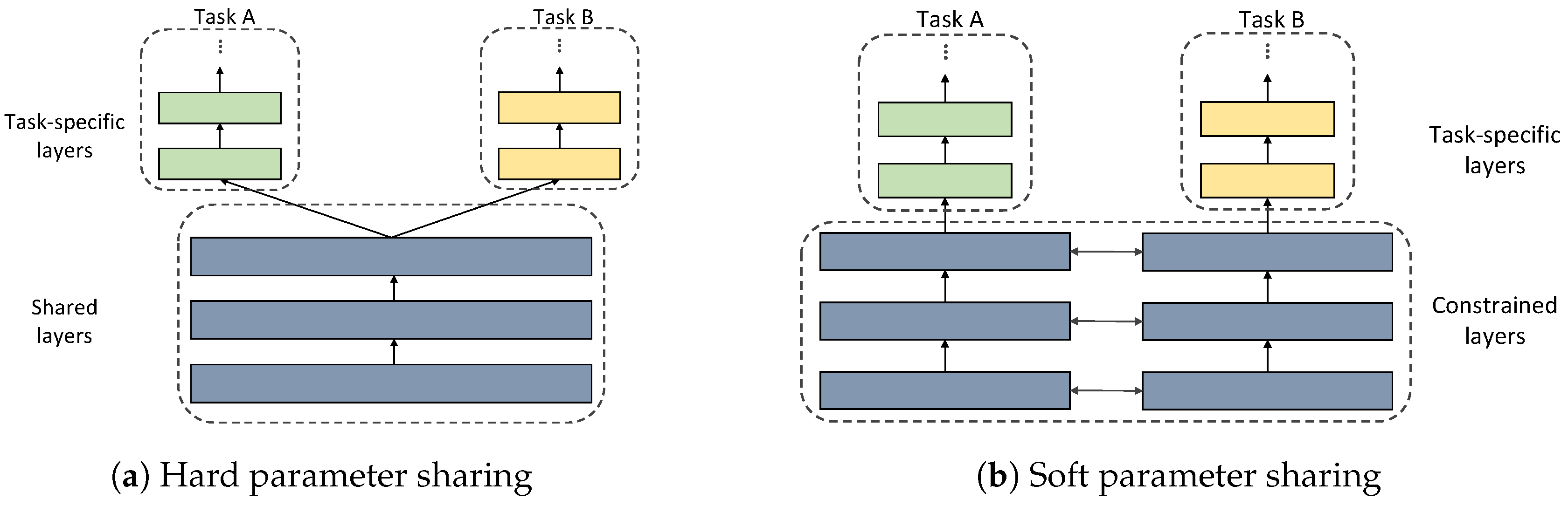
Compared with joint model-based estimation of SOC and SOH, significantly less work has been done for joint data-driven estimation. However, prior knowledge tells us that when we estimate SOC and SOH at the same time, these two states are dependent on each other, especially SOC on SOH. There should be some shared information about the two states, which can be captured by a neural network and thus benefit the model. A deep learning paradigm of this type is called multi-task learning (MTL), which has been successfully applied across a variety of applications of machine learning [48,49], such as natural language processing [50] and computer vision [51]. Research has shown that applying MTL techniques brings improved learning efficiency, better generalization, less risk of overfitting, and higher resource efficiency to deep learning models [48,49]. 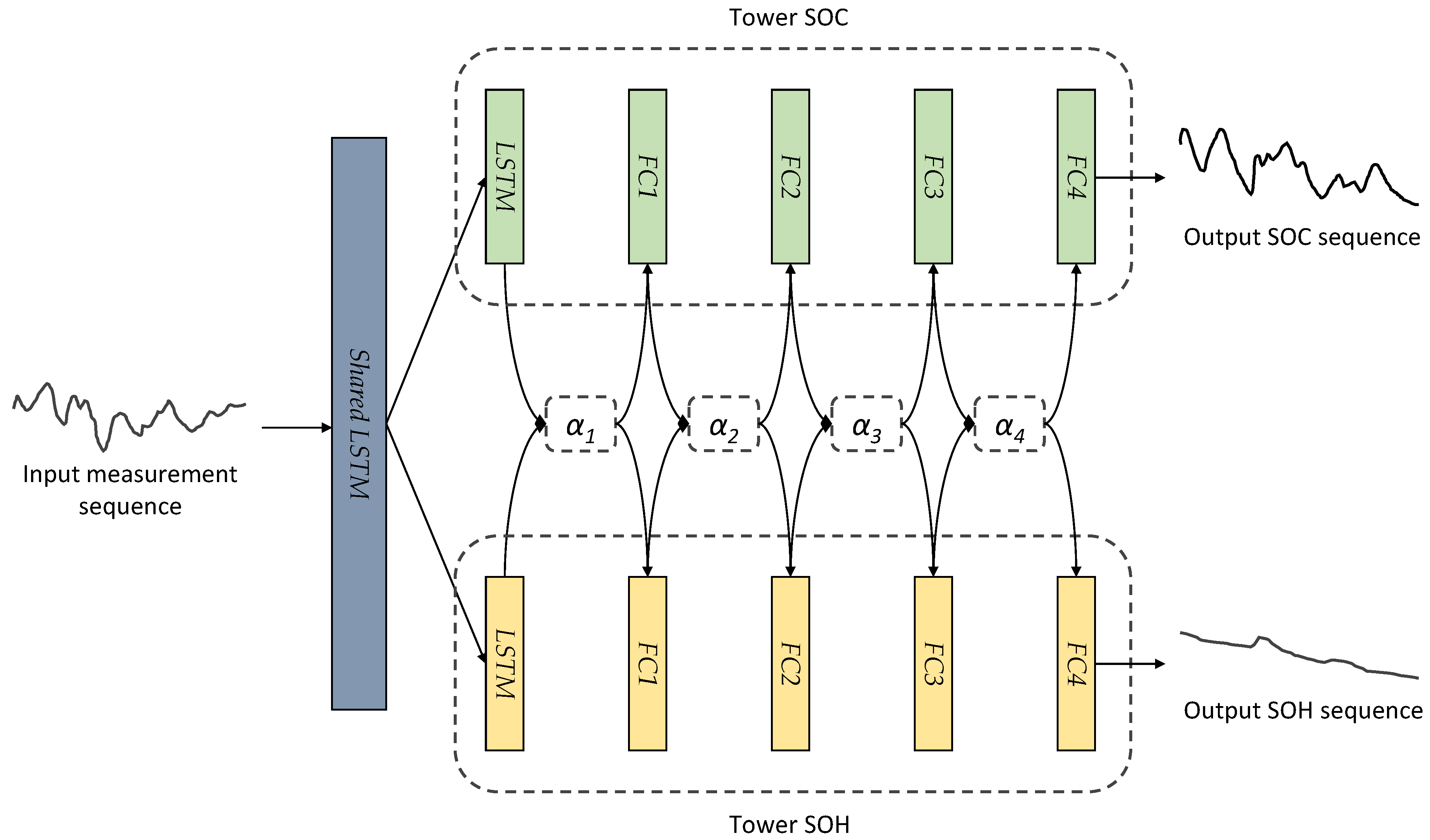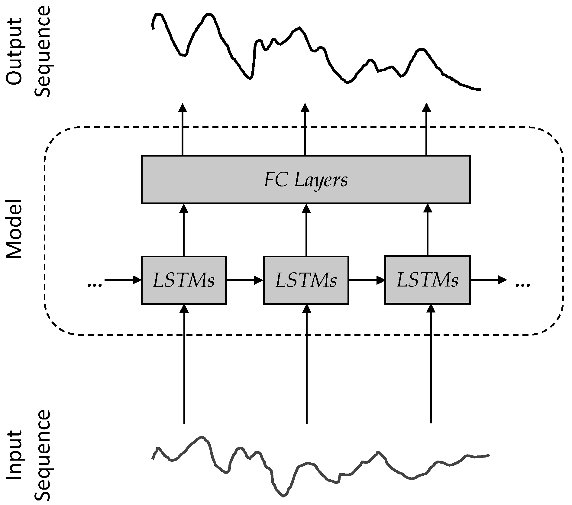There have also been several applications of MTL to batteries [52,53,54]. However, to the best of our knowledge, there is still no precedent work applying MTL to the joint estimation of SOC and SOH, the two most important states of a battery cell. Furthermore, we deem the implementation of such joint estimation of SOC and SOH much more meaningful for real-world applications if the model allows for an online estimation, meaning the estimation is causal and conducted in real time based solely on historical and current information without interrupting the normal usage of the battery. Therefore, in this paper, we propose a novel data-driven approach for joint SOC and SOH online estimation of lithium-ion batteries utilizing multi-task learning. The proposed model takes the differing time scales in the dynamics of SOC and SOH into consideration, delivering accurate estimation results. It is suitable for online applications through synchronous sequence-to-sequence implementation.

The rest of this paper is structured as follows: Section 2 introduces the proposed model with the applied methodology explained in detail; Section 3 displays the acquired results of the proposed model under different experiments, which are then analyzed and interpreted in Section 4. Finally, Section 5 summarizes the achieved results of this paper and gives a short outlook of our future work.

2. Methodology

2.1. Multi-Task Learning

Typically, multi-task learning in deep learning can be categorized into two kinds: hard parameter sharing and soft parameter sharing, as shown in Figure 1 [48].

Hard parameter sharing, the most common strategy in MTL, primarily involves sharing the bottom hidden layers between all tasks while each task keeps several task-specific layers to itself [48]. In hard parameter sharing, tasks share the same layers for the representation of fundamental features. This architecture significantly reduces the risk of overfitting and increases the generalization ability of the model across different tasks by learning the more general representation. Hard parameter sharing is resource-efficient in parameter usage because of the reduction in the total number of parameters in the model. This approach is simple and easy to implement at the same time. However, such an architecture forces the same basic feature representation on all tasks, which is only optimal if all the tasks are closely related. The lack of flexibility also inevitably leads to limited performance. Conversely, soft parameter sharing allows each task to have its own model and parameter set. Instead of directly sharing the bottom layers, soft parameter sharing encourages the models to learn the shared information by regularizing the parameters of different tasks [48]. This method brings great flexibility into the model as each task is allowed to keep the task-specific information while benefiting from the sharing between different tasks. It is especially useful when a balance needs to be reached between learning tasks specifically and collectively. Of course, such an architecture is typically more resource-intensive and complex regarding the model and training procedures. Furthermore, finding the right degree of parameter sharing across the tasks is a challenging task in itself. Thus, we combine the principles of both hard and soft parameter sharing, which is tailored for our task of joint SOC and SOH estimation, aiming for an efficient, flexible model with simple training procedures and an optimized extent of information sharing across the two tasks. Figure 2 displays the architecture of the proposed model, which will be explained in detail in the rest of this section.

2.2. Model Overview

As shown in Figure 2, the proposed model consists of a shared bottom layer for both tasks and one task-specific tower for each task. The shared bottom layer is a shared LSTM layer, and both towers consist of one task-specific LSTM layer and four fully connected (FC) layers. The model takes measurement sequences, including voltage, current, and temperature, as input and outputs the estimated SOC sequence and SOH sequence. At time step k, the input of the model is defined as ${\mathit{x}}_{\mathit{k}}=[U_k,I_k,T_k]$, and the output is defined as ${\mathit{y}}_{\mathit{k}}=[{\widehat{SOC}}_k,{\widehat{SOH}}_k]$. In addition, the task-specific LSTM for SOH estimation is initialized using the battery’s initial SOH of the time sequence modulated by two FC layers, which makes the model’s estimation possible at any life stage of the battery cell. The task-specific layers, or the towers of both tasks, are aligned and connected with the so-called cross-stitch units [55]. Take the cross-stitch unit ${\alpha }_1$ for example, this takes the output of the two task-specific LSTM layers as input, and the output will be fed to the next layer of each task. The underlying assumption of the proposed model is that the fundamental battery dynamics for estimating SOC and SOH should be the same. However, from the fundamental dynamics to the high-level output of SOC and SOH, the intermediate features of both tasks should have less and less shared information. The use of a shared LSTM layer underpins the model with a common representation that captures the fundamental battery dynamics intrinsic to both SOC and SOH. This shared representation leverages the intrinsic connection between SOC and SOH by sharing the underlying temporal patterns and dependencies to both tasks. At the same time, cross-stitch units are introduced to enable the flow of the shared information from one task to another while keeping the unique information of each task to itself, offering the necessary flexibility to tailor the model to the unique aspects of each task. As will be elucidated in the rest of the section, the cross-stitch units are trainable, meaning the parameters will be updated during model training to optimize the performance of the model, and the model can determine to what extent the sharing will be itself. The introduction of the cross-stitch units ensures that while the model benefits from a shared understanding of fundamental battery behavior, it also retains the capacity to adapt to the specific nuances and requirements of each task individually. The shared LSTM layer and the two task-specific LSTM layers are used to capture the shared and task-specific temporal features for SOC and SOH estimation, and the FC layers will map the temporal features to the corresponding SOC and SOH of each time step.

2.3. Long Short-Term Memory

In the field of deep learning, RNNs are often used for time series processing, while common feedforward neural networks take only the current input data as the model’s input, RNNs take the input data of the current time step and the output of the previous time step as the model’s input so that they can learn the temporal dynamic behavior of the input sequence. As a refined RNN model, LSTM [56] introduces a gate mechanism into its architecture. This mechanism is used to manage the information flow within the unit, determining which information should be retained and which should be discarded, ensuring the key information from earlier in the sequence is not lost. This innovation effectively addresses the shortcomings of vanilla RNN, particularly its struggle with capturing long-term dependencies. By doing so, LSTM enhances the network’s ability to process longer sequences and convey the entire sequence’s information with greater precision. At the same time, LSTM also solves the problem of vanishing gradient with vanilla RNNs. Figure 3 shows the internal structure of a single LSTM unit [57].

In Figure 3, ${\mathit{c}}_{\mathit{t}},{\mathit{h}}_{\mathit{t}},{\mathit{f}}_{\mathit{t}},{\mathit{i}}_{\mathit{t}},{\tilde{\mathit{c}}}_{\mathit{t}}$, and ${\mathit{o}}_{\mathit{t}}$ stand for cell state, hidden state, forget gate, input gate, cell gate, and output gate, respectively, at time step t. At each time step, the LSTM unit takes three inputs: cell state from previous moment ${\mathit{c}}_{\mathit{t}-\mathbf{1}}$, hidden state from previous moment ${\mathit{h}}_{\mathit{t}-\mathbf{1}}$, and input data of current moment ${\mathit{x}}_{\mathit{t}}$. At the same time, it produces two outputs: cell state of current moment ${\mathit{c}}_{\mathit{t}}$ and hidden state of current moment ${\mathit{h}}_{\mathit{t}}$. The mapping equations are written as follows:

$${\mathit{i}}_{\mathit{t}}=\sigma ({\mathit{W}}_{\mathit{i}}{\mathit{x}}_{\mathit{t}}+{\mathit{U}}_{\mathit{i}}{\mathit{h}}_{\mathit{t}-\mathbf{1}}+{\mathit{b}}_{\mathit{i}})$$

(4)

$${\mathit{f}}_{\mathit{t}}=\sigma ({\mathit{W}}_{\mathit{f}}{\mathit{x}}_{\mathit{t}}+{\mathit{U}}_{\mathit{f}}{\mathit{h}}_{\mathit{t}-\mathbf{1}}+{\mathit{b}}_{\mathit{f}})$$

(5)

$${\mathit{o}}_{\mathit{t}}=\sigma ({\mathit{W}}_{\mathit{o}}{\mathit{x}}_{\mathit{t}}+{\mathit{U}}_{\mathit{o}}{\mathit{h}}_{\mathit{t}-\mathbf{1}}+{\mathit{b}}_{\mathit{o}})$$

(6)

$${\tilde{\mathit{c}}}_{\mathit{t}}=\sigma ({\mathit{W}}_{\mathit{g}}{\mathit{x}}_{\mathit{t}}+{\mathit{U}}_{\mathit{g}}{\mathit{h}}_{\mathit{t}-\mathbf{1}}+{\mathit{b}}_{\mathit{g}})$$

(7)

$${\mathit{c}}_{\mathit{t}}={\mathit{f}}_{\mathit{t}}\odot {\mathit{c}}_{\mathit{t}-\mathbf{1}}+{\mathit{i}}_{\mathit{t}}\odot {\tilde{\mathit{c}}}_{\mathit{t}}$$

(8)

$${\mathit{h}}_{\mathit{t}}={\mathit{o}}_{\mathit{t}}\odot tanh\left({\mathit{c}}_{\mathit{t}}\right)$$

(9)

Equation (8) displays how the current cell state ${\mathit{c}}_{\mathit{t}}$ is updated: it is a combination of the previous cell state after the forgetting and the current input information after selection. With the current cell state ${\mathit{c}}_{\mathit{t}}$, the current hidden state can be calculated with the selection by the output gate as in Equation (9). Because of the advantages of LSTM, it is used to capture the temporal features in our work.

2.4. Cross-Stitch Unit

Cross-stitch units and cross-stitch networks were first proposed in computer vision in order to learn an optimal combination of shared and task-specific representations [55]. In essence, a cross-stitch unit is a matrix with trainable coefficients that describe the contribution of one task to another. In the case of n tasks, a cross-stitch unit would have the structure as shown in Figure 4.

The cross-stitch unit receives input features from n tasks and then linearly combines them using the cross-stitch coefficients. If we denote the input features of the i-th task as ${\mathit{x}}_{\mathit{i}}$ and the output combined features for the i-th task as ${\tilde{\mathit{x}}}_{\mathit{i}}$, then the forward pass process can be written as follows:

$$\left[\begin{array}{c}{\tilde{\mathit{x}}}_{\mathbf{1}}\\ {\tilde{\mathit{x}}}_{\mathbf{2}}\\ ⋮\\ {\tilde{\mathit{x}}}_{\mathit{n}}\end{array}\right]=\left[\begin{array}{cccc}{\alpha }_{11}& {\alpha }_{12}& \cdots & {\alpha }_{1n}\\ {\alpha }_{21}& {\alpha }_{22}& \cdots & {\alpha }_{2n}\\ ⋮& ⋮& \ddots & ⋮\\ {\alpha }_{n1}& {\alpha }_{n2}& \cdots & {\alpha }_{nn}\end{array}\right]\left[\begin{array}{c}{\mathit{x}}_{\mathbf{1}}\\ {\mathit{x}}_{\mathbf{2}}\\ ⋮\\ {\mathit{x}}_{\mathit{n}}\end{array}\right]$$

(10)

where ${\alpha }_{ij}$ represents the contribution of features from task j to task i. As mentioned above, the coefficients of the cross-stitch unit are trainable, meaning they will converge to the optimized extent of sharing across the tasks to ensure the best performance of the model. If we denote the total loss of the network as L, then the backpropagation process can be written as follows:

$$\left[\begin{array}{c}\frac{\partial L}{\partial {\mathit{x}}_{\mathbf{1}}}\\ \frac{\partial L}{\partial {\mathit{x}}_{\mathbf{2}}}\\ ⋮\\ \frac{\partial L}{\partial {\mathit{x}}_{\mathit{n}}}\end{array}\right]=\left[\begin{array}{cccc}{\alpha }_{11}& {\alpha }_{21}& \cdots & {\alpha }_{n1}\\ {\alpha }_{12}& {\alpha }_{22}& \cdots & {\alpha }_{n2}\\ ⋮& ⋮& \ddots & ⋮\\ {\alpha }_{1n}& {\alpha }_{2n}& \cdots & {\alpha }_{nn}\end{array}\right]\left[\begin{array}{c}\frac{\partial L}{\partial {\tilde{\mathit{x}}}_{\mathbf{1}}}\\ \frac{\partial L}{\partial {\tilde{\mathit{x}}}_{\mathbf{2}}}\\ ⋮\\ \frac{\partial L}{\partial {\tilde{\mathit{x}}}_{\mathit{n}}}\end{array}\right]$$

(11)

$$\left[\begin{array}{cccc}\frac{\partial L}{\partial {\alpha }_{11}}& \frac{\partial L}{\partial {\alpha }_{12}}& \cdots & \frac{\partial L}{\partial {\alpha }_{1n}}\\ \frac{\partial L}{\partial {\alpha }_{21}}& \frac{\partial L}{\partial {\alpha }_{22}}& \cdots & \frac{\partial L}{\partial {\alpha }_{2n}}\\ ⋮& ⋮& \ddots & ⋮\\ \frac{\partial L}{\partial {\alpha }_{n1}}& \frac{\partial L}{\partial {\alpha }_{n2}}& \cdots & \frac{\partial L}{\partial {\alpha }_{nn}}\end{array}\right]=\left[\begin{array}{c}\frac{\partial L}{\partial {\tilde{\mathit{x}}}_{\mathbf{1}}}\\ \frac{\partial L}{\partial {\tilde{\mathit{x}}}_{\mathbf{2}}}\\ ⋮\\ \frac{\partial L}{\partial {\tilde{\mathit{x}}}_{\mathit{n}}}\end{array}\right]\left[\begin{array}{cccc}{\mathit{x}}_{\mathbf{1}}& {\mathit{x}}_{\mathbf{2}}& \cdots & {\mathit{x}}_{\mathit{n}}\end{array}\right]$$

(12)

In our case, we have a two-task scenario. IF we denote the two tasks as A and B, respectively, then the i-th cross-stitch unit used here can be written as:

$${\alpha }_i=\left[\begin{array}{cc}{\alpha }_{AA}^i& {\alpha }_{AB}^i\\ {\alpha }_{BA}^i& {\alpha }_{BB}^i\end{array}\right]$$

(13)

For simplicity, we refer to ${\alpha }_{AA}$ and ${\alpha }_{BB}$ as non-sharing coefficients, and refer to ${\alpha }_{AB}$ and ${\alpha }_{BA}$ as sharing coefficients.

2.5. Multi-Scale Online Estimation

In general, time-series processing tasks can be categorized into sequence-to-class and sequence-to-sequence [58]. Different types of sequence processing require different types of implementation. As indicated by its name, sequence-to-class means the model takes a sequence of data as input and produces the classification result of the sequence. For example, tasks like sentiment analysis. For the implementation of a sequence-to-class task, the model should read the whole input sequence data before making the final decision. As for sequence-to-sequence, there are two ways to implement this approach: asynchronous sequence-to-sequence and synchronous sequence-to-sequence. Both take a sequence of data as input but produce a sequence as output as well. Synchronous sequence-to-sequence is often used in sequence labeling tasks like part-of-speech tagging and named entity recognition. At each time step, the model’s current output is considered as a part of the output sequence. In the case of synchronous sequence-to-sequence, the input and output sequences are of the same length. Conversely, synchronous sequence-to-sequence, often in the form of an encoder–decoder model, is widely used in tasks like text translation. The input sequence is fed into the encoder model, and the output is then passed into the decoder part to generate the output sequence. As is intuitive in real-world applications, the length of the input and output sequence is usually different. In the scenario of battery state estimation, it is usually expected that the model can output the real-time estimation of the current time step, especially for SOC estimation tasks. Furthermore, in real applications, the length of the input sequence, namely the running duration of the estimation system, is usually unknown. In other words, a model that is only able to produce the estimation results after the whole input sequence is completely taken is not of much use in real-world applications. Therefore, the proposed model is implemented as synchronous sequence-to-sequence. Figure 5 is a schematic diagram of such an implementation. At time step k, the LSTM layers take ${\mathit{x}}_{\mathit{k}}=[U_k,I_k,T_k]$ as input, the output of which will then be fed into the fully connected layers to map into the output of the current time step ${\mathit{y}}_{\mathit{k}}=[{\widehat{SOC}}_k,{\widehat{SOH}}_k]$. In other words, the elements of the output sequence $\mathit{Y}=[{\mathit{y}}_{\mathbf{1}},{\mathit{y}}_{\mathbf{2}},{\mathit{y}}_{\mathbf{3}},...,{\mathit{y}}_{\mathit{T}}]$ and the input sequence $\mathit{X}=[{\mathit{x}}_{\mathbf{1}},{\mathit{x}}_{\mathbf{2}},{\mathit{x}}_{\mathbf{3}},...,{\mathit{x}}_{\mathit{T}}]$ are one-to-one in time steps. The output of each time step is also causal in this case, meaning it only takes past and current input information into consideration.

In addition, as mentioned above, the change in SOC is usually much more dynamic than that of SOH, which means while the estimation of SOC needs to be updated on a very frequent basis, the estimation of SOH can be updated less frequently in order to save computation effort without causing much inaccuracy in the results. Consequently, we introduce a multi-scale temporal architecture into our model: the shared bottom layer and the tower of SOC estimation are implemented with a sampling period of 1 s, while the tower of SOH estimation is implemented with a sampling period of 3600 s. This multi-scale temporal architecture allows for an efficient allocation of computational resources. By setting a higher sampling rate for SOC estimation, the model is capable of capturing the rapid fluctuations and providing real-time updates, which is crucial given the dynamic nature of SOC changes. In contrast, the significantly lower sampling rate for the SOH estimation tower fits the relatively slow process of battery aging, allowing the model to reach a balance between optimized computational effort and long-term accuracy.

2.6. Dataset and Preprocessing

Data are the foundation of a successful machine learning model. In a typical BMS, the directly measured data include current, voltage, and temperature. For SOC estimation, it is more meaningful to focus on short-term dynamic data, while for SOH estimation, long-term aging data are the main focus. Therefore, cyclic aging data is usually used for the training of SOH estimation models in research, while SOC estimation models are usually trained on battery data under dynamic load profiles because of the fast-changing nature of SOC and the practicality compared to real-world scenarios [34]. Consequently, the appropriate training data for a joint SOC and SOH estimation model are expected to contain dynamic load profiles as well as long-term aging. Battery cells can come in different shapes, e.g., cylindrical [59], prismatic [60], and pouch cells [61]. Cylindrical cells are the most widely used shape for lithium-ion batteries because of the advantages of a large amount of experience in their manufacture and a good lifespan. Common cylindrical cell sizes include 18650, 21700, and 26650, where the first two digits denote the diameter of the cylindrical cell and the following two digits denote its length. As one of the most common sizes of cylindrical cells, 18650 cells have not only been used in various applications of lithium-ion batteries but also are often chosen for the development of novel cell chemistry [62]. Therefore, in order to meet the requirements of the training of our joint SOC and SOH estimation model and present it in the case of the most commonly used type of lithium-ion batteries for a convincing result, we utilize our previously published open-source dataset [7]. The dataset is comprised of thirty LG 18650HE4 lithium-ion battery cells, whose specifications are displayed in

Table 1. LG 18650HE4 cell specifications.

Parameter	Data
Nominal Capacity	$2.5$ Ah
Nominal Voltage	$3.6$ V
Charging Cutoff Voltage	$4.2$ V
Discharging Cutoff Voltage	$2.5$ V
Max. Charging Current	4 A
Max. Discharging Current	20 A

.

The whole dataset covers the cyclic aging scenarios with a variety of stress factors: temperatures of 23 °C, 25 °C, and 45 °C, depths of discharge (DODs) of 30%, 70%, and 100%, and mean SOCs of 35%, 50%, and 65%. The batteries were tested with a Neware battery tester with a voltage limit of 10 V and a current range of ±10 A. To control the ambient temperature, a Memmert oven and a Binder temperature chamber were used. Two out of the thirty cells were aged using dynamic profiles under room temperature 23 °C and a mixture of DODs, which are used for the training, validation, and testing of the proposed model. As shown in Figure 6, the used dataset is divided into two parts: dynamic cycling and checkup tests. For the dynamic cycling part, the used load profiles were generated from the federal urban driving schedule (FUDS) using the so-called random pulse method [63]. This method segments the FUDS cycle into small pieces and then concatenates the pieces into our desired load profile stochastically, which ensures that the generated profiles are dynamic and have the same intrinsic features as the original FUDS cycle. At the same time, the generated cycles of different DODs are constructed differently due to the stochastic concatenation, which brings more diversity into the dataset. The generated dynamic cycles cover different cycles of 25%, 50%, 75%, 80%, and 95% DOD. Capacity tests are interspersed in the dynamic cycling around every ten equivalent full cycles (EFCs). The cyclic aging is regularly interrupted by a set of checkup tests. The checkup tests consist of a capacity test, an OCV measurement, a modified hybrid pulse power characterization (HPPC), and an extra dynamic cycling part for validation purposes, which has a different pattern to that of the cyclic aging data. The reference SOC is calculated using coulomb counting. The reference SOH is calculated using the capacity test data and then interpolated over the whole dataset based on EFCs. It is worth mentioning that because of test device logging errors, the dynamic cycles of 25% DOD were poorly sampled, which caused a great error in the calculation of the reference SOC. Therefore, this small part of the data was deprecated. For further details of the dataset, please refer to [7].

To ensure a constant sampling rate, the raw dynamic cycling data was resampled with a sampling rate of 1 Hz. Afterward, the resampled dataset was split randomly into training, validation, and test sets in the ratio of 6:2:2. The training set is used for the learning of the model, namely updating the model’s parameters to minimize the loss. However, each trained model is subject to one set of hyperparameters, which is why the validation set is required to test the model’s performance during training in order to fine-tune the model’s hyperparameters. It also offers a metric to prevent overfitting during the training phase. After the training and fine-tuning are done, the test set is used to test the best model’s performance. The test set should be completely independent and not used in the training or validation process so that it can provide an unbiased evaluation of the final model’s generalization ability on the target tasks in real-world scenarios. After the data split was done, a sliding window approach was used as data augmentation for the training set. Subsets of the original time-series data were created by sliding a fixed-size window over the dataset, which significantly increased the available amount of training data. It also provided a more comprehensive view of the time series, which improved the model’s robustness to different patterns in the data. The window size was set to 24 h, with the overlap ratio being 0.5. Min-max normalization was applied to the dataset, adjusting the measurements of different scales to the same scale. In our work, the input data was normalized into the range [0, 1] using the following formulas [64]:

$$x_{std}=\frac{x-x_{min}}{x_{max}-x_{min}}$$

(14)

$$x_{scaled}=x_{std}·(max-min)+min$$

(15)

where x is the original value of a feature, $x_{min}$ is the minimum value of the feature, $x_{max}$ is the maximum value of the feature, $max$ and $min$ are the expected range, and $x_{scaled}$ is the normalized value of the feature. Implementing normalization as preprocessing has many benefits: it adjusts the scales of different features into the same range so that each feature contributes approximately proportionately to the network; it can also improve the network’s performance and accelerate the convergence of the network during training [65]. It is worth mentioning that the validation data and test data should be normalized using the minimum and maximum feature values from the training set so that no information leakage happens.

3. Results

The exact architecture specifications of the proposed model are displayed in

Table 2. Network architecture specifications.

Layer	Input Size	Output Size
Shared LSTM	3	256
Task-Specific LSTM (both)	256	256
FC Layer 1 (both)	256	256
FC Layer 2 (both)	256	128
FC Layer 3 (both)	128	64
FC Layer 4 (both)	64	1

.

For the training of the model, a loss function needs to be designed. In this work, we mainly exploited the mean squared error (MSE) between the estimates and ground-truth values of SOC and SOH. The calculation of MSE is defined as follows:

$$MSE(\mathit{y},\widehat{\mathit{y}})=\frac{1}{n}\sum _{i=1}^n{(y_i-{\widehat{y}}_i)}^2$$

(16)

During the training, assisting loss terms to penalize large changing rates and non-monotonicity of the estimated SOH were experimented with as well. However, no evident improvement was found. The applied batch size varies from 4 to 8 and 16 because of the limited GPU memory. However, for a fair comparison of the following results, the same number of iterations was applied, namely 4500. The training process integrates automatic fine-tuning of the learning rates using the open-source hyperparameter optimization framework Optuna [66] and the use of the early stopping technique, which is why sometimes the actual number of trained iterations is slightly less than 4500. For the evaluation of the results, mean absolute error and root mean square error were used, which are defined as follows:

$$MAE(\mathit{y},\widehat{\mathit{y}})=\frac{1}{n}\sum _{i=1}^n|y_i-{\widehat{y}}_i|$$

(17)

$$RMSE(\mathit{y},\widehat{\mathit{y}})=\sqrt{\frac{1}{n}\sum _{i=1}^n{(y_i-{\widehat{y}}_i)}^2}$$

(18)

MAE averages every sample point equally, offering an intuitive and understandable metric, especially since both SOC and SOH are in the range of [0, 1]. RMSE is more sensitive to outliers since the square operation amplifies their influence.

3.1. Loss Weighting

As mentioned above, the loss function consists of the MSE of SOC estimation and SOH estimation. However, the change in the estimated SOC and SOH have different ranges, and the difficulty that the model has in learning the two tasks is also different. Therefore, finding a good way to balance the loss in both tasks is crucial. We experimented with in total three different weighting methods for the loss function, namely empirical weighting, uncertainty weighting, and dynamic weight average (DWA).

3.1.1. Empirical Weighting

The most intuitive way for loss weighting would be to observe the values of both losses and try to balance them with a weight hyperparameter. We call this approach empirical weighting. In this case, the loss function can be written as follows:

$$L=L_{SOC}+w·L_{SOH}$$

(19)

The empirical weighting method is straightforward to implement using the predefined hyperparameter only and offers explicit and manual control over the influence of each task. However, since the weight is fixed during training, it cannot adapt to changes in task-learning dynamics. We experimented with different weight hyperparameters and compared the results. The weight hyperparameter $w=5$ evidently offers advantages over the other candidates.

3.1.2. Uncertainty Weighting

Uncertainty weighting was first proposed by [67]. The authors introduced the concept of homoscedastic task uncertainty as a metric for loss weighting. The derived loss function is as follows:

$$L=\frac{1}{2{\sigma }_{SOC}^2}{L}_{SOC}+\frac{1}{2{\sigma }_{SOH}^2}{L}_{SOH}+log{\sigma }_{SOC}+log{\sigma }_{SOH}$$

(20)

where $\sigma$ is the model’s observation noise parameter of either task and is learnable during training. With this method, the weights are adjusted automatically. The log terms can also be seen as regularization terms: without the log terms, the model will automatically only focus on the easier task to minimize the loss and ignore the other. In other words, the regularization terms make it possible for the weight hyperparameter in empirical weighting to become trainable. However, this approach is much more complex to implement than empirical weighting, as it involves the learning of extra parameters.

3.1.3. Dynamic Weight Average

Ref. [68] proposed the weighting scheme dynamic weight average. The loss weighting is updated from iteration to iteration based on the rate of change of the loss for each task. The given formulas are as follows:

$$w_k(t-1)=\frac{L_k(t-1)}{L_k(t-2)}$$

(21)

$${\lambda }_k\left(t\right)=\frac{K{e}^{\frac{w_k(t-1)}{T}}}{\sum _i{e}^{\frac{w_i(t-1)}{T}}}$$

(22)

where $k\in \{SOC,SOH\}$, $w_k$ is the calculated relative descending rate, T controls the softness of the weighting, and K controls the sum of the weights. DWA continuously updates the weights based on real-time training dynamics. The slower the loss in one task decreases, the larger the portion that task will be assigned during the next iteration. However, due to the highly dynamic changes in weightings, oscillations in learning and potentially unstable training dynamics might be introduced.

We experimented with the aforementioned three weighting methods with the same model architecture and hyperparameters, using in all cases the training paradigm of end-to-end training, which will be explained later in this section. The MAE and RMSE of the estimation results are shown in

Table 3. Results with different weighting methods.

Weighting Method	SOC		SOH
	MAE [%]	RMSE [%]	MAE [%]	RMSE [%]
Empirical Weighting	0.743	0.961	0.062	0.080
Uncertainty Weighting	1.470	1.777	0.177	0.204
Dynamic Weight Average	1.107	1.407	0.119	0.151

. On all metrics, empirical weighting shows the smallest error. Taking the simple implementation of this method into consideration, all later training and results are based on the weighting method of empirical weighting with $w=5$.

3.2. Training Paradigm

The cross-stitch units are interpretable: the linear combination of the task-specific features means information sharing between the two tasks. When it comes to the training of such networks, an intuitive question would be: is it better to train the model with cross-stitch units integrated from the beginning so that the layers have better expression ability, or should we let the towers of both tasks first learn their own task-specific representations and then add cross-stitch units to combine them [55]? We experimented with both training paradigms, namely end-to-end training and fine-tuning with cross-stitch units. In end-to-end training, we directly train both towers jointly with cross-stitch units from scratch, where the cross-stitch units function more like a medium for the information flow between both tasks. The two towers are less distinct since they are trained to serve both tasks from the beginning. In fine-tuning with cross-stitch units, we first train both towers separately, then add cross-stitch units for fine-tuning. Here, the cross-stitch units carry more responsibility in combining the features since both towers focus more on their own tasks. For a fair comparison, we kept the number of total iterations the same. We trained the model end-to-end for 4500 iterations. For the second training paradigm, we first pre-trained the model without cross-stitch units for 1341 iterations, then fine-tuned the model for the rest of the iterations. Three test case examples of the model’s performance under both training paradigms are shown in Figure 7.

Table 4. Results with different training paradigms.

Training Paradigm	SOC		SOH
	MAE [%]	RMSE [%]	MAE [%]	RMSE [%]
End-to-End Training	0.743	0.961	0.062	0.080
Fine-Tuning with Cross-Stitch Units	0.554	0.759	0.063	0.078
Separate (Single-Task Model)	1.324	1.717	0.147	0.185

displays the model’s performance on the whole test set. In general, the fine-tuned model displays better results in SOC estimation and the RMSE in SOH estimation, while the end-to-end trained model displays lower MAE in SOH estimation, which means the SOH estimation of the fine-tuned model is slightly less accurate than that of the end-to-end trained model but with fewer outliers. However, since the difference in the error is negligible, it is safe to conclude that the training paradigm of fine-tuning with cross-stitch units brings better performance to the proposed model.

The learning processes of the four cross-stitch units with both training paradigms are shown in Figure 8. Note that ${\alpha }_{AA}^i$ and ${\alpha }_{BB}^i$ are the non-sharing coefficients and were initialized as 1, while ${\alpha }_{AB}^i$ and ${\alpha }_{BA}^i$ are the sharing coefficients and were initialized as 0. The greater the absolute values of the sharing coefficients, the stronger the sharing between both tasks. An absolute value of zero of a sharing coefficient means that there is no information shared for the corresponding tasks at the corresponding layer. As can be seen from the plots, the sharing takes place to a larger extent in the fine-tuned model than in the end-to-end trained model. As mentioned above, the underlying reason is that the cross-stitch units in the end-to-end trained model function more as a medium to allow for the information flow between the two towers during the training, while those in the fine-tuned model aim at combining the task-specific features of the pre-trained towers. In other words, in the fine-tuned model, the cross-stitch units are required to have greater sharing coefficients, while the existence of cross-stitch units itself is already sufficient in the end-to-end trained model for an optimized performance. Generally, it can also be observed that the absolute values of the sharing coefficients tend to decrease as the cross-stitch units get closer to the final output layers, which is intuitive since the higher the level of features, the less shared information there is. Furthermore, it can be observed that ${\alpha }_{AB}^i$ is usually greater than ${\alpha }_{BA}^i$ in the sense of absolute value, which complies with our prior knowledge as well: the determination of SOC is more dependent on SOH than the determination of SOH on SOC. The four ${\alpha }_{AA}^i$ in the end-to-end trained model turned out to be updated to significantly greater than 1. We assume that this functions as compensation for the learning rate of the SOC tower.

3.3. Comparison with Single-Task Model

In addition, we trained a single-task model with the same architecture but without sharing for comparison. The single-task model consists of two completely separate networks, one for SOC estimation and one for SOH estimation. For simplicity, the two subnetworks were encapsulated in one training process, but of course with different learning rates. The same number of iterations is kept as well. The performance of the single-task model is shown in Table 4. The MAE and RMSE of both SOC and SOH estimations are more than doubled than those of the fine-tuned model. The isolation of the two estimation towers in the single-task model significantly decreases the neural network’s performance, considering the single-task model has exactly the same architecture as the multi-task model except for one extra LSTM layer to account for the shared LSTM layer in the multi-task model. Furthermore, we compared the training process of the single-task model and the end-to-end trained multi-task model, as shown in Figure 9. The single-task model reached convergence at around 1950 iterations, while the proposed model reached convergence at around 450 iterations already. Therefore, it can be concluded that the introduction of cross-stitch units accelerates the training of the neural network.

3.4. Generalization Test on SOC Estimation

Although the SOH of every sample in the dataset is different, the SOCs of the samples share a similar pattern of changes. In order to test how the model generalizes on the task of SOC estimation, the aforementioned extra dynamic cycling part for validation purposes in each checkup test is used. These extra dynamic cycles were constructed differently to those in the training set and thus are eligible to test the model’s generalization ability. However, these cycles are not sufficiently long to display an evident aging effect of the cells. Therefore, they were only used for the test of SOC estimation.

Figure 10 displays the generalization test results under three test cases, in which in test case 1, the cell has an almost full SOH, while in test cases 2 and 3, the cell has aged significantly. As shown in the figures, the single-task model displays the largest estimation error in all three test cases, which becomes more evident as the SOH decreases. All three models are able to converge to an accurate SOC estimation rapidly at the beginning of the inference, which should be attributed to the capability of the LSTM layers. It can be observed that the error is generally higher in the lower SOC range, which is possibly caused by the accumulation of estimation errors during the partial dynamic profiles. Nonetheless, the proposed model under both training paradigms is able to maintain its accuracy in these cases.

Table 5. Generalization test on SOC estimation.

Training Paradigm	SOC
	MAE [%]	RMSE [%]
End-to-End Training	0.924	1.560
Fine-Tuning with Cross-Stitch Units	0.786	1.270
Separate (Single-Task Model)	1.690	2.355

shows the MAE and RMSE of SOC estimation, respectively, for the end-to-end trained model, the cross-stitch units fine-tuned model, and the single-task model. Not surprisingly, the cross-stitch units fine-tuned model showed the best performance on both metrics, where the error itself is also relatively low considering the test profiles include a variety of dynamic partial cycles and charging cases and, therefore, have high complexity. The results show that the proposed model under both training paradigms is able to generalize not only on the SOH estimation task but also on the SOC estimation task.

4. Discussion

4.1. Model

The proposed model lies within the framework of multi-task learning, combining the principles of hard parameter sharing and soft parameter sharing. To capture the fundamental battery dynamics, a shared bottom layer is utilized for both tasks. For the learning of the task-specific features, two towers, namely task-specific layers for SOC and SOH, are established. Cross-stitch units are introduced in the model to enable information sharing between the two towers, which simply carry out a linear combination and can be updated during the training. To the best of our knowledge, this is the first attempt to apply multi-task learning to joint SOC and SOH estimation. The proposed model utilizes LSTM layers, a refined type of RNN, to capture the temporal features of the time series, which further enables the possibility of an online application of the model with synchronous sequence-to-sequence implementation. The model can process the initial SOH information and use it to initialize the SOH tower, meaning it is able to function at any given life stage of the battery cell. It is especially practical for real-world application cases where the real SOH can be calibrated from time to time via complete discharging. Due to the separate tower structure, the proposed model is able to carry out SOC and SOH estimation tasks in different time scales by updating the towers with different frequencies. To sum up, the proposed model achieves information sharing between the two tasks with a minimized cost in resources and is perfectly designed for real-world application scenarios.

4.2. Training

For the training of the model, dynamic aging profiles from our previously published open-source dataset are used [7]. For multi-task learning models, the weighting of the loss terms is especially important for a balanced, optimized training of the tasks. In this work, three different weighting methods are mentioned and tested. Although the most straightforward approach, namely empirical weighting, shows the best performance, it is possible that with skillful tuning and more effort invested, other more sophisticated weighting methods could outperform the empirical weighting method. Two different training paradigms have been presented in this paper, namely end-to-end training and first pre-training then fine-tuning with cross-stitch units. The focus of the cross-stitch units’ role is different in the two cases: the cross-stitch units can either function more as a medium for information flow or be more responsible for combining task-specific features. The results have shown that the model performs better when the cross-stitch units are only used for fine-tuning after the two towers have learned the task-specific representations explicitly in a separate way. The evolution of the cross-stitch units during training also complies with our prior knowledge.

4.3. Performance

Test results of the proposed model under the two training paradigms and a corresponding single-task model are presented in the paper. Results show that the proposed model outperforms the traditional single-task model without information sharing and is able to generalize on different SOCs and SOHs. However, we noticed a great challenge during evaluation: even though the two tasks are implemented in different time scales to account for the difference between the dynamics of SOC and SOH, the estimated SOH still displays a high degree of fluctuation, which decreases the accuracy. We assume that this is caused by the mutual influence of how the SOH changes and by how much: unlike SOC, SOH decreases monotonically most of the time and often slowly and in a much smaller range. Different attempts have been made to overcome the problem. First, we tried to rescale the range of the output SOH, which reduces the error in SOH estimation but with the cost of increasing the error in SOC estimation. We also tried to apply a filtering algorithm as postprocessing of the output. However, no significant improvement was observed due to the restriction of causality for the online estimation system. Nonetheless, we believe there will be an appropriate approach to deal with such differences in dynamics during training or as postprocessing that is able to further improve the model’s performance. This will be further investigated in the future.

5. Conclusions

In this paper, we proposed for the first time a deep learning model for joint online estimation of SOC and SOH of lithium-ion batteries utilizing multi-task learning. More specifically, the proposed model combines the principles of hard parameter sharing and a simple soft parameter sharing approach, namely cross-stitching. With the cross-stitch units, the model is able to learn the optimal extent of information sharing between both tasks during the training. The proposed model is able to achieve an accurate estimation of SOC and SOH in online applications. In addition, the feature of multi-scale estimation is introduced in the implementation of the model, aiming for a resource-efficient system. During the work, we have established that it is particularly difficult to overcome the problems caused by the difference in SOC and SOH dynamics. In addition to more advanced weighting methods for the design of the loss function, it would be meaningful to explore transforms of the model’s input and output and tricks for the training of the model as well in order to achieve a dynamic SOC estimation and a smooth SOH estimation simultaneously. Postprocessing methods to filter the estimated SOH is also a possible way forward if causality is ensured. To date, all the data for training, validation, and testing have been acquired at room temperature; it would be beneficial to generalize the model on different temperatures. In conclusion, we believe our work is a meaningful attempt at data-driven joint estimation of SOC and SOH, and we hope more future work will be done within its scope.

References

1. Campagna, N.; Castiglia, V.; Miceli, R.; Mastromauro, R.A.; Spataro, C.; Trapanese, M.; Viola, F. Battery Models for Battery Powered Applications: A Comparative Study. Energies 2020, 13, 4085. [Google Scholar] [CrossRef]
2. Wang, Y.; Liu, B.; Li, Q.; Cartmell, S.; Ferrara, S.; Deng, Z.D.; Xiao, J. Lithium and Lithium Ion Batteries for Applications in Microelectronic Devices: A Review. J. Power Sources 2015, 286, 330–345. [Google Scholar] [CrossRef]
3. Saldaña, G.; San Martín, J.I.; Zamora, I.; Asensio, F.J.; Oñederra, O. Analysis of the Current Electric Battery Models for Electric Vehicle Simulation. Energies 2019, 12, 2750. [Google Scholar] [CrossRef]
4. Ali, M.U.; Zafar, A.; Nengroo, S.H.; Hussain, S.; Alvi, M.J.; Kim, H.J. Towards a Smarter Battery Management System for Electric Vehicle Applications: A Critical Review of Lithium-Ion Battery State of Charge Estimation. Energies 2019, 12, 446. [Google Scholar] [CrossRef]
5. Li, Y.; Li, K.; Liu, X.; Li, X.; Zhang, L.; Rente, B.; Sun, T.; Grattan, K.T. A Hybrid Machine Learning Framework for Joint SOC and SOH Estimation of Lithium-Ion Batteries Assisted with Fiber Sensor Measurements. Appl. Energy 2022, 325, 119787. [Google Scholar] [CrossRef]
6. Diao, W.; Jiang, J.; Zhang, C.; Liang, H.; Pecht, M. Energy State of Health Estimation for Battery Packs Based on the Degradation and Inconsistency. Energy Procedia 2017, 142, 3578–3583. [Google Scholar] [CrossRef]
7. Neupert, S.; Kowal, J. Model-Based State-of-Charge and State-of-Health Estimation Algorithms Utilizing a New Free Lithium-Ion Battery Cell Dataset for Benchmarking Purposes. Batteries 2023, 9, 364. [Google Scholar] [CrossRef]
8. Chen, L.; Lü, Z.; Lin, W.; Li, J.; Pan, H. A New State-of-Health Estimation Method for Lithium-Ion Batteries through the Intrinsic Relationship between Ohmic Internal Resistance and Capacity. Measurement 2018, 116, 586–595. [Google Scholar] [CrossRef]
9. Cui, Z.; Dai, J.; Sun, J.; Li, D.; Wang, L.; Wang, K. Hybrid Methods Using Neural Network and Kalman Filter for the State of Charge Estimation of Lithium-Ion Battery. Math. Probl. Eng. 2022, 2022, 1–11. [Google Scholar] [CrossRef]
10. Chen, C.; Xiong, R.; Yang, R.; Shen, W.; Sun, F. State-of-Charge Estimation of Lithium-Ion Battery Using an Improved Neural Network Model and Extended Kalman Filter. J. Clean. Prod. 2019, 234, 1153–1164. [Google Scholar] [CrossRef]
11. Dang, X.; Yan, L.; Jiang, H.; Wu, X.; Sun, H. Open-Circuit Voltage-Based State of Charge Estimation of Lithium-Ion Power Battery by Combining Controlled Auto-Regressive and Moving Average Modeling with Feedforward-Feedback Compensation Method. Int. J. Electr. Power Energy Syst. 2017, 90, 27–36. [Google Scholar] [CrossRef]
12. Ng, K.S.; Moo, C.S.; Chen, Y.P.; Hsieh, Y.C. Enhanced Coulomb Counting Method for Estimating State-of-Charge and State-of-Health of Lithium-Ion Batteries. Appl. Energy 2009, 86, 1506–1511. [Google Scholar] [CrossRef]
13. How, D.N.T.; Hannan, M.A.; Hossain Lipu, M.S.; Ker, P.J. State of Charge Estimation for Lithium-Ion Batteries Using Model-Based and Data-Driven Methods: A Review. IEEE Access 2019, 7, 136116–136136. [Google Scholar] [CrossRef]
14. Shrivastava, P.; Soon, T.K.; Idris, M.Y.I.B.; Mekhilef, S. Overview of Model-Based Online State-of-Charge Estimation Using Kalman Filter Family for Lithium-Ion Batteries. Renew. Sustain. Energy Rev. 2019, 113, 109233. [Google Scholar] [CrossRef]
15. Jiang, Y.; Zhang, J.; Xia, L.; Liu, Y. State of Health Estimation for Lithium-Ion Battery Using Empirical Degradation and Error Compensation Models. IEEE Access 2020, 8, 123858–123868. [Google Scholar] [CrossRef]
16. Li, W.; Fan, Y.; Ringbeck, F.; Jöst, D.; Han, X.; Ouyang, M.; Sauer, D.U. Electrochemical Model-Based State Estimation for Lithium-Ion Batteries with Adaptive Unscented Kalman Filter. J. Power Sources 2020, 476, 228534. [Google Scholar] [CrossRef]
17. Yu, Z.; Huai, R.; Xiao, L. State-of-Charge Estimation for Lithium-Ion Batteries Using a Kalman Filter Based on Local Linearization. Energies 2015, 8, 7854–7873. [Google Scholar] [CrossRef]
18. Liu, X.; Fan, X.; Wang, L.; Wu, J. State of Charge Estimation for Power Battery Base on Improved Particle Filter. World Electr. Veh. J. 2022, 14, 8. [Google Scholar] [CrossRef]
19. Jiang, C.; Taylor, A.; Duan, C.; Bai, K. Extended Kalman Filter Based Battery State of Charge(SOC) Estimation for Electric Vehicles. In Proceedings of the 2013 IEEE Transportation Electrification Conference and Expo (ITEC), Metro Detroit, MI, USA, 16–19 June 2013; pp. 1–5. [Google Scholar] [CrossRef]
20. Chen, Z.; Fu, Y.; Mi, C.C. State of Charge Estimation of Lithium-Ion Batteries in Electric Drive Vehicles Using Extended Kalman Filtering. IEEE Trans. Veh. Technol. 2013, 62, 1020–1030. [Google Scholar] [CrossRef]
21. Imran, R.M.; Li, Q.; Flaih, F.M.F. An Enhanced Lithium-Ion Battery Model for Estimating the State of Charge and Degraded Capacity Using an Optimized Extended Kalman Filter. IEEE Access 2020, 8, 208322–208336. [Google Scholar] [CrossRef]
22. Zhang, F.; Liu, G.; Fang, L. Battery State Estimation Using Unscented Kalman Filter. In Proceedings of the 2009 IEEE International Conference on Robotics and Automation, Kobe, Japan, 12–17 May 2009; pp. 1863–1868. [Google Scholar] [CrossRef]
23. Xing, J.; Wu, P. State of Charge Estimation of Lithium-Ion Battery Based on Improved Adaptive Unscented Kalman Filter. Sustainability 2021, 13, 5046. [Google Scholar] [CrossRef]
24. He, Z.; Chen, D.; Pan, C.; Chen, L.; Wang, S. State of Charge Estimation of Power Li-ion Batteries Using a Hybrid Estimation Algorithm Based on UKF. Electrochim. Acta 2016, 211, 101–109. [Google Scholar] [CrossRef]
25. Hu, X.; Sun, F.; Zou, Y. Estimation of State of Charge of a Lithium-Ion Battery Pack for Electric Vehicles Using an Adaptive Luenberger Observer. Energies 2010, 3, 1586–1603. [Google Scholar] [CrossRef]
26. Ning, B.; Cao, B.; Wang, B.; Zou, Z. Adaptive Sliding Mode Observers for Lithium-Ion Battery State Estimation Based on Parameters Identified Online. Energy 2018, 153, 732–742. [Google Scholar] [CrossRef]
27. Chen, N.; Zhang, P.; Dai, J.; Gui, W. Estimating the State-of-Charge of Lithium-Ion Battery Using an H-Infinity Observer Based on Electrochemical Impedance Model. IEEE Access 2020, 8, 26872–26884. [Google Scholar] [CrossRef]
28. Wu, T.; Liu, S.; Wang, Z.; Huang, Y. SOC and SOH Joint Estimation of Lithium-Ion Battery Based on Improved Particle Filter Algorithm. J. Electr. Eng. Technol. 2022, 17, 307–317. [Google Scholar] [CrossRef]
29. Yu, Q.; Xiong, R.; Yang, R.; Pecht, M.G. Online Capacity Estimation for Lithium-Ion Batteries through Joint Estimation Method. Appl. Energy 2019, 255, 113817. [Google Scholar] [CrossRef]
30. Azis, N.A.; Joelianto, E.; Widyotriatmo, A. State of Charge (SoC) and State of Health (SoH) Estimation of Lithium-Ion Battery Using Dual Extended Kalman Filter Based on Polynomial Battery Model. In Proceedings of the 2019 6th International Conference on Instrumentation, Control, and Automation (ICA), Bandung, Indonesia, 31 July–2 August 2019; pp. 88–93. [Google Scholar] [CrossRef]
31. Gao, Y.; Liu, K.; Zhu, C.; Zhang, X.; Zhang, D. Co-Estimation of State-of-Charge and State-of- Health for Lithium-Ion Batteries Using an Enhanced Electrochemical Model. IEEE Trans. Ind. Electron. 2022, 69, 2684–2696. [Google Scholar] [CrossRef]
32. Wang, Y.; Tian, J.; Sun, Z.; Wang, L.; Xu, R.; Li, M.; Chen, Z. A Comprehensive Review of Battery Modeling and State Estimation Approaches for Advanced Battery Management Systems. Renew. Sustain. Energy Rev. 2020, 131, 110015. [Google Scholar] [CrossRef]
33. Ren, Z.; Du, C. A Review of Machine Learning State-of-Charge and State-of-Health Estimation Algorithms for Lithium-Ion Batteries. Energy Rep. 2023, 9, 2993–3021. [Google Scholar] [CrossRef]
34. Dos Reis, G.; Strange, C.; Yadav, M.; Li, S. Lithium-Ion Battery Data and Where to Find It. Energy AI 2021, 5, 100081. [Google Scholar] [CrossRef]
35. Álvarez Antón, J.C.; García Nieto, P.J.; Blanco Viejo, C.; Vilán Vilán, J.A. Support Vector Machines Used to Estimate the Battery State of Charge. IEEE Trans. Power Electron. 2013, 28, 5919–5926. [Google Scholar] [CrossRef]
36. Liu, Z.; Zhao, J.; Wang, H.; Yang, C. A New Lithium-Ion Battery SOH Estimation Method Based on an Indirect Enhanced Health Indicator and Support Vector Regression in PHMs. Energies 2020, 13, 830. [Google Scholar] [CrossRef]
37. Hu, X.; Li, S.E.; Yang, Y. Advanced Machine Learning Approach for Lithium-Ion Battery State Estimation in Electric Vehicles. IEEE Trans. Transp. Electrif. 2016, 2, 140–149. [Google Scholar] [CrossRef]
38. Hannan, M.A.; Lipu, M.S.H.; Hussain, A.; Saad, M.H.; Ayob, A. Neural Network Approach for Estimating State of Charge of Lithium-Ion Battery Using Backtracking Search Algorithm. IEEE Access 2018, 6, 10069–10079. [Google Scholar] [CrossRef]
39. Wu, J.; Zhang, C.; Chen, Z. An Online Method for Lithium-Ion Battery Remaining Useful Life Estimation Using Importance Sampling and Neural Networks. Appl. Energy 2016, 173, 134–140. [Google Scholar] [CrossRef]
40. Chemali, E.; Kollmeyer, P.J.; Preindl, M.; Emadi, A. State-of-Charge Estimation of Li-ion Batteries Using Deep Neural Networks: A Machine Learning Approach. J. Power Sources 2018, 400, 242–255. [Google Scholar] [CrossRef]
41. Chemali, E.; Kollmeyer, P.J.; Preindl, M.; Ahmed, R.; Emadi, A. Long Short-Term Memory Networks for Accurate State-of-Charge Estimation of Li-ion Batteries. IEEE Trans. Ind. Electron. 2018, 65, 6730–6739. [Google Scholar] [CrossRef]
42. Bhattacharjee, A.; Verma, A.; Mishra, S.; Saha, T.K. Estimating State of Charge for xEV Batteries Using 1D Convolutional Neural Networks and Transfer Learning. IEEE Trans. Veh. Technol. 2021, 70, 3123–3135. [Google Scholar] [CrossRef]
43. You, G.W.; Park, S.; Oh, D. Diagnosis of Electric Vehicle Batteries Using Recurrent Neural Networks. IEEE Trans. Ind. Electron. 2017, 64, 4885–4893. [Google Scholar] [CrossRef]
44. Fan, Y.; Xiao, F.; Li, C.; Yang, G.; Tang, X. A Novel Deep Learning Framework for State of Health Estimation of Lithium-Ion Battery. J. Energy Storage 2020, 32, 101741. [Google Scholar] [CrossRef]
45. Shen, S.; Sadoughi, M.; Chen, X.; Hong, M.; Hu, C. A Deep Learning Method for Online Capacity Estimation of Lithium-Ion Batteries. J. Energy Storage 2019, 25, 100817. [Google Scholar] [CrossRef]
46. Hu, P.; Tang, W.F.; Li, C.H.; Mak, S.L.; Li, C.Y.; Lee, C.C. Joint State of Charge (SOC) and State of Health (SOH) Estimation for Lithium-Ion Batteries Packs of Electric Vehicles Based on NSSR-LSTM Neural Network. Energies 2023, 16, 5313. [Google Scholar] [CrossRef]
47. Huang, H.; Bian, C.; Wu, M.; An, D.; Yang, S. A Novel Integrated SOC–SOH Estimation Framework for Whole-Life-Cycle Lithium-Ion Batteries. Energy 2024, 288, 129801. [Google Scholar] [CrossRef]
48. Ruder, S. An Overview of Multi-Task Learning in Deep Neural Networks. arXiv 2017, arXiv:1706.05098. [Google Scholar]
49. Thung, K.H.; Wee, C.Y. A Brief Review on Multi-Task Learning. Multimed. Tools Appl. 2018, 77, 29705–29725. [Google Scholar] [CrossRef]
50. Chen, S.; Zhang, Y.; Yang, Q. Multi-Task Learning in Natural Language Processing: An Overview. arXiv 2021, arXiv:2109.09138. [Google Scholar] [CrossRef]
51. Vandenhende, S. Multi-Task Learning for Visual Scene Understanding. arXiv 2022, arXiv:2203.14896. [Google Scholar]
52. Li, W.; Zhang, H.; Van Vlijmen, B.; Dechent, P.; Sauer, D.U. Forecasting Battery Capacity and Power Degradation with Multi-Task Learning. Energy Storage Mater. 2022, 53, 453–466. [Google Scholar] [CrossRef]
53. Bao, X.; Liu, Y.; Liu, B.; Liu, H.; Wang, Y. Multi-State Online Estimation of Lithium-Ion Batteries Based on Multi-Task Learning. Energies 2023, 16, 3002. [Google Scholar] [CrossRef]
54. Che, Y.; Zheng, Y.; Wu, Y.; Lin, X.; Li, J.; Hu, X.; Teodorescu, R. Battery States Monitoring for Electric Vehicles Based on Transferred Multi-Task Learning. IEEE Trans. Veh. Technol. 2023, 72, 10037–10047. [Google Scholar] [CrossRef]
55. Misra, I.; Shrivastava, A.; Gupta, A.; Hebert, M. Cross-Stitch Networks for Multi-task Learning. arXiv 2016, arXiv:1604.03539. [Google Scholar]
56. Hochreiter, S.; Schmidhuber, J. Long Short-Term Memory. Neural Comput. 1997, 9, 1735–1780. [Google Scholar] [CrossRef]
57. Kong, Z.; Cui, Y.; Xia, Z.; Lv, H. Convolution and Long Short-Term Memory Hybrid Deep Neural Networks for Remaining Useful Life Prognostics. Appl. Sci. 2019, 9, 4156. [Google Scholar] [CrossRef]
58. Recurrent Neural Networks RNN. 2024. Available online: https://paddlepedia.readthedocs.io/en/latest/tutorials/sequence_model/rnn.html (accessed on 28 March 2024).
59. Baazouzi, S.; Feistel, N.; Wanner, J.; Landwehr, I.; Fill, A.; Birke, K.P. Design, Properties, and Manufacturing of Cylindrical Li-Ion Battery Cells—A Generic Overview. Batteries 2023, 9, 309. [Google Scholar] [CrossRef]
60. Gitzendanner, R.; Russell, P.; Marsh, C.; Marsh, R. Design and Development of A 20 Ah Li-ion Prismatic Cell. J. Power Sources 1999, 81–82, 847–852. [Google Scholar] [CrossRef]
61. Yi, X.; Rao, A.M.; Zhou, J.; Lu, B. Trimming the Degrees of Freedom via a K+ Flux Rectifier for Safe and Long-Life Potassium-Ion Batteries. Nano-Micro Lett. 2023, 15, 200. [Google Scholar] [CrossRef]
62. Yi, X.; Fu, H.; Rao, A.M.; Zhang, Y.; Zhou, J.; Wang, C.; Lu, B. Safe Electrolyte for Long-Cycling Alkali-Ion Batteries. Nat. Sustain. 2024, 7, 326–337. [Google Scholar] [CrossRef]
63. Kellner, Q.; Hosseinzadeh, E.; Chouchelamane, G.; Widanage, W.D.; Marco, J. Battery Cycle Life Test Development for High-Performance Electric Vehicle Applications. J. Energy Storage 2018, 15, 228–244. [Google Scholar] [CrossRef]
64. Pedregosa, F.; Varoquaux, G.; Gramfort, A.; Michel, V.; Thirion, B.; Grisel, O.; Blondel, M.; Müller, A.; Nothman, J.; Louppe, G.; et al. Scikit-Learn: Machine Learning in Python. arXiv 2018, arXiv:1201.0490. [Google Scholar]
65. Sola, J.; Sevilla, J. Importance of Input Data Normalization for the Application of Neural Networks to Complex Industrial Problems. IEEE Trans. Nucl. Sci. 1997, 44, 1464–1468. [Google Scholar] [CrossRef]
66. Akiba, T.; Sano, S.; Yanase, T.; Ohta, T.; Koyama, M. Optuna: A Next-generation Hyperparameter Optimization Framework. arXiv 2019, arXiv:1907.10902. [Google Scholar]
67. Kendall, A.; Gal, Y.; Cipolla, R. Multi-Task Learning Using Uncertainty to Weigh Losses for Scene Geometry and Semantics. arXiv 2018, arXiv:1705.07115. [Google Scholar]
68. Liu, S.; Johns, E.; Davison, A.J. End-to-End Multi-Task Learning with Attention. arXiv 2019, arXiv:1803.10704. [Google Scholar]
Figure 1. The two basic types of MTL.
Batteries 10 00171 g001
Figure 2. Overview of the proposed model’s architecture.
Batteries 10 00171 g002
Figure 3. Internal structure of an LSTM unit.
Batteries 10 00171 g003
Figure 4. Cross-stitch unit for n tasks.
Batteries 10 00171 g004
Figure 5. Synchronous sequence-to-sequence implementation of the model.
Batteries 10 00171 g005
Figure 6. Demonstration of dataset samples.
Batteries 10 00171 g006
Figure 7. Estimation results under three test cases (test case 1: row 1–2; test case 2: row 3–4; test case 3: row 5–6). Columns from left to right: SOC estimation of the end-to-end trained model, SOH estimation of the end-to-end trained model, SOC estimation of the fine-tuned model, and SOH estimation of the fine-tuned model. Odd-numbered rows show the plots of ground truths and estimates of each test case. Even-numbered rows show the plots of the absolute error of the estimations of the corresponding test case.
Batteries 10 00171 g007
Figure 8. Learning processes of the cross-stitch units. Left column: end-to-end trained; right column: fine-tuned with cross-stitch units. From top to bottom: α 1 , α 2 , α 3 , α 4 .
Batteries 10 00171 g008
Figure 9. Training processes of multi-task model and single-task model.
Batteries 10 00171 g009
Figure 10. Generalization test results under three test cases (test case 1: row 1; test case 2: row 2; test case 3: row 3). Left column: comparison between the ground-truth values and estimations; right column: comparison between absolute errors.
Batteries 10 00171 g010