Abstract
The accurate state of health (SOH) estimation of lithium-ion batteries (LIBs) during operation is crucial to ensure optimal performance, prolonging battery life and preventing unexpected failure or safety hazards. This work presents a storage- and performance-optimised deep learning approach to estimate the capacity-based SOH of LIBs using raw sensor data from partial charging curves under constant current condition. The proposed model is based on a combination of a one-dimensional convolutional and long short-term memory neural network, and processes time, voltage, and incremental capacity of partial charging curves as time series. The model is cross-validated on different ageing scenarios, reaching an overall MAE = 0.418% and RMSE = 0.531%, promising an accurate SOH estimation of LIBs under varying usage and environmental conditions in a real-world application.
1. Introduction
The urgent need to reduce greenhouse gas emissions and combat climate change has provoked the rapid adoption of renewable energy systems and electrification of the transportation sector. LIBs have gained prominence in both of these areas in recent years. They are used as stationary storage to compensate for the intermittent nature of renewable energy sources by quickly and efficiently storing excess energy during periods of high production and releasing it during low- or no-generation periods [1]. In the transportation sector, LIBs are widely used as traction batteries in electromobility due to their high energy density and power capability [2].
However, like any electrochemical energy storage system, LIBs undergo degradation over time. The SOH is a widely adopted metric to assess the degradation of LIBs, typically expressed as a percentage value that represents the remaining useful life of the battery, and is commonly based either on the inner resistance or on the remaining capacity relative to their initial values [3].
This work presents a methodology to estimate the capacity-based SOH, defined as follows
where is the nominal and C the actual capacity. The accurate estimation of the SOH during operation is crucial for ensuring optimal performance, prolonging lifespan, and preventing unexpected failures or safety hazards of battery systems. Due to the non-linear degradation, its complex underlying mechanisms and their interactions [3], accurate online SOH estimation is a non-trivial task. Different methodologies can be found in the literature for evaluating the SOH of LIBs, with the most basic and accurate technique being Coulomb counting while performing a complete discharge of the battery.
Other more sophisticated methods like incremental capacity analysis (ICA) [4,5], differential voltage analysis [6], and electrochemical impedance spectroscopy [7,8] are widely discussed in the literature for SOH evaluation under laboratory conditions. All three methods are rather suitable for online SOH estimation due to the need of a unique current profile, high measurement accuracy, and further processing of the acquired data.
Recently discussed approaches for online SOH estimation can be roughly categorised into model-based [9,10,11,12] and data-driven [13,14,15,16,17,18,19,20,21,22,23,24] methods. Model-based algorithms are built on a parametrised battery model, usually in a recursive implementation such as Kalman filters. The underlying battery model can be either an equivalent circuit model [9,10] or an electrochemical model [11,12], where the latter is rather suitable for online SOH estimation due to its high computational complexity. The accuracy of model-based algorithms highly depends on the choice of the underlying battery model and its parametrisation, both of which require a high level of domain specific knowledge.
Data-driven methods, on the other hand, have the ability to map measured input data to labelled output data, being able to model complex and non-linear relationships without any information about the underlying physical or chemical processes. The estimation quality can vary with the selection of the underlying algorithm and the choice, quality, and amount of training data.
Many data-driven approaches for SOH estimation can be found in the literature ranging from Gaussian process regression [16,17], support vector machines [18,19] over deep learning [15,20,21,23], and other neural network approaches [14,22,24] commonly using extracted features from voltage, current, and/or temperature measurements as input data.
Zheng et al. [25] analysed the change in terminal voltage during constant current charging for various SOHs and showed a significant change in inclination over time with falling SOH, making them a suitable base as an input feature for data-driven algorithms. They predicted the SOH with an RMSE = 1.9% based on the linear assumption of charged capacity within a fixed voltage range.
Wei et al. [14] used features like peak height, area, and width from filtered incremental capacity (IC) curves during constant current charging to predict SOH with a multilayer perceptron (MLP) neural network. They achieved an MAE < 0.24% for partial charging starting at Vinit < 3.7 V. The main limitation of this approach is the computationally expensive IC curve filtering and feature extraction.
Liu et al. [20] utilised the integrated voltage and current over time from charging curves as input features and estimated the SOH using a long short-term memory (LSTM) neural network. The model achieved a MAE = 0.5747% and RMSE = 0.5623%. However, the extraction and processing of input features introduces additional computational complexity to the overall algorithm.
Rzepka et al. [22] estimated the SOH from samples of voltage, temperature, and cumulative current using a MLP neural network, reaching MAE = 1.1 and MSE = 2.52. Caused by the cumulative current, this approach incorporates historical data to estimate SOH, thereby potentially overlooking individual or abnormal battery ageing phenomena.
Li et al. [15] used voltage and time samples of partial charging curves under constant current condition as input features. They proposed a deep neural network (DNN) consisting of four bi-directional long short-term memory (Bi-LSTM) layers to process the partial charging curve as time series, hence being able to process raw sensor data of a BMS without any preprocessing or feature engineering.
The relatively complex topology of the proposed DNN demands a certain amount of storage and computational power, making it unsuitable for low-budget embedded devices associated with most modern BMS. Furthermore, all of the above-mentioned approaches do not consider different ageing scenarios in their datasets and, therefore, cannot validate the robustness of the proposed algorithms against different ageing mechanisms caused by varying environmental conditions or usage of LIBs in a real-world application.
This work is motivated by bridging the aforementioned research gap by building a dataset with eleven different ageing scenarios and refining the methodology proposed by Li et al. [15] by developing a storage-optimised DNN model with low computational complexity supplemented by the inclusion of IC as an input feature to enhance estimation accuracy. The proposed DNN is based on a one-dimensional convolutional neural network (1-D CNN) combined with two subsequent LSTM layers and processes time series of raw sensor data (time, voltage, IC) of partial charging curves under constant current condition to estimate the SOH of LIBs. The model will undergo cross-validation over different ageing scenarios to asses the robustness of the methodology against different ageing mechanisms. The actual storage occupancy, computational complexity, and prediction performance is evaluated by deploying the proposed model on a commercially available embedded device.
The subsequent sections are structured as follows: Section 2 presents the dataset and the features utilised for model training and validation. Section 3 provides an overview of the neural networks employed and presents the topology of the applied DNN. Section 4 provides the validation results under various aspects along with their corresponding discussions. Lastly, Section 5 presents the main conclusions drawn from this work.
2. Dataset
The dataset used for this work consists of ageing data collected from 22 Bexel INR18650-2600 cells, obtained from in-house experiments conducted as part of the LioBat project. The active materials are lithium-nickel-manganese-cobalt-oxide (NMC) for the positive electrode and carbon (C) for the negative electrode. The specification of the cell is given in Table 1.

Table 1.
Cell specifications [26].
2.1. Experimental
In order to represent different usage of batteries within the dataset, eleven different ageing scenarios were applied. They encompass a spectrum of different cycling strategies and pure calendric ageing. Each ageing scenario is applied to two individual cells. An overview of the different scenarios is shown in Table 2.
Table 2.
Ageing scenarios.
Within Scenario 1, the cells are cycled with a depth of discharge (DOD) of 100% and a current rate of 1C for both charging and discharging. Scenario 1 can be seen as a standard for accelerated ageing tests and is commonly featured in datasets used for SOH estimation. Scenarios 2–4 focus on partial cycling at different states of charge (SOC). Specifically, Scenario 2 cycles between an SOC of 5% and 35%, Scenario 3 between 35% and 65%, and Scenario 4 between 65% and 95%, all utilising a current rate of 1C for both charging and discharging. Scenario 5 is similar to Scenario 1 but considers a higher load which is reflected by a discharge current rate of 2C. Scenarios 6 and 7 replicate the cycling conditions of Scenarios 1 and 5, respectively but are conducted at an elevated temperature of 45 °C, reflecting the use of LIBs under different thermal conditions. Scenario 11 represents dynamic load conditions using the federal urban driving schedule (FUDS) as a discharge current profile. The current profile is scaled to a maximum current rate of 1C and is applied repetitively until the cell is fully discharged. The current rate for charging is constant and equals 1C. Scenarios 8–10 address calendric ageing, where cells are stored at different SOCs under an environmental temperature of 35 °C.
Within the experiments, characterisation tests were carried out at regular intervals of 50 equivalent full cycles for cells subjected to cycling and a 30-day interval for cells undergoing calendric ageing. The characterisation tests include determining the actual capacity and acquiring of a full charging curve under constant current condition.
They were conducted under a controlled temperature environment of 35 °C. The measurements and cycling were carried out using a Neware CT-4008-5V6A battery testing system (BTS) (Neware, Singapore).
The tests proceeded in three phases, each of them separated by a 30 min rest time. The first phase brings the cell to an initial fully charged state by a charging process with a constant current of 1C until the cut-off voltage is reached, followed by a constant voltage step until the current attains a level of C/100. The second phase is oriented to determine the discharge capacity by using Coulomb counting while discharging the cell with a constant current of 1C until the terminal voltage reaches the discharge cut-off voltage. After the capacity determination, the cell is fully discharged by applying a constant voltage until the current again attains a level of C/100. A third and final phase acquires the full charging curve by charging the cell with a current of 1C until the charge cut-off voltage is reached.
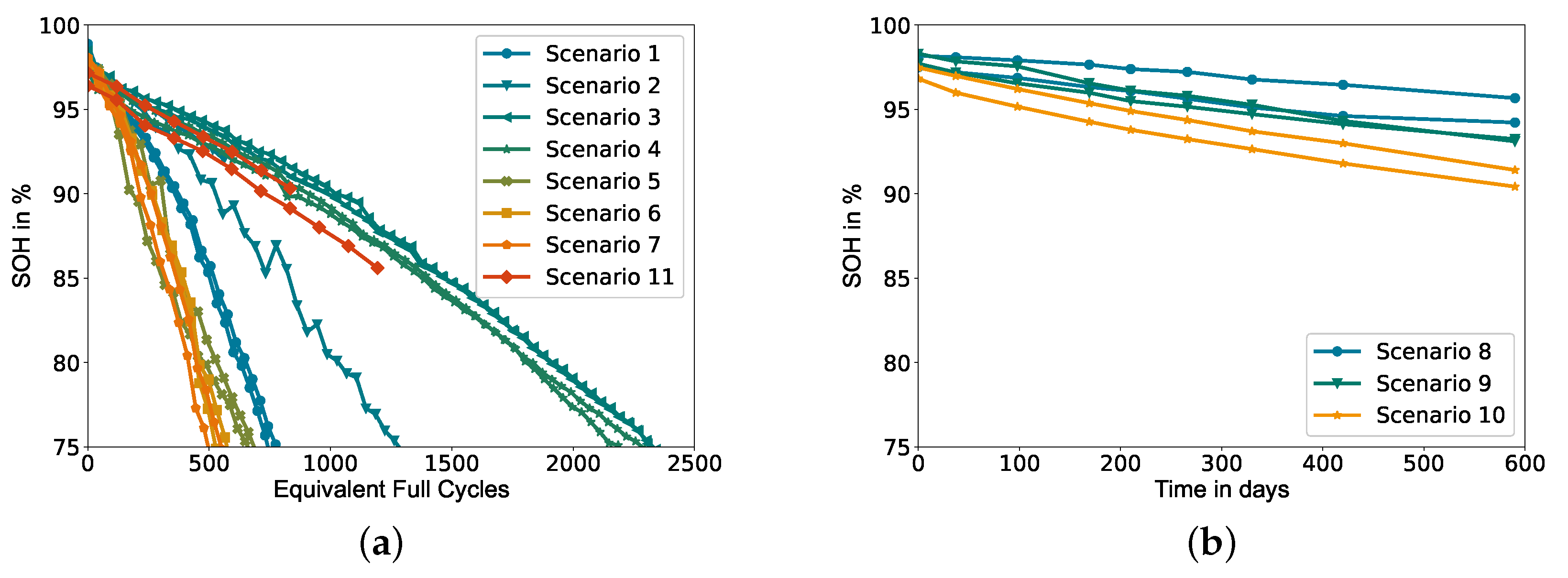
Figure 1 shows the trajectory of capacity degradation of all cells present in the dataset. All cycled cells are aged until they reach 75% of their nominal capacity. The experiments involving calendric aged cells and Scenario 11 are terminated prematurely due to time constraints. Furthermore, cell numbers 3 (Scenario 2) and 21 (Scenario 11) fail during the experiment, exhibiting an abrupt drop in terminal voltage to zero volts. Cell number 4 (scenario 2) shows an unexpectedly accelerated ageing rate compared to analogue scenarios. Nevertheless, its data are kept in the dataset to demonstrate the robustness of the proposed methodology, even in cases of abnormal ageing behaviours.

Figure 1.
Capacity decay of all cells contained in the dataset: (a) SOH of cycle-aged cells over equivalent full cycles. (b) SOH of calendric-aged cells over time in days.
2.2. Feature Selection and Data Preprocessing
The proposed model uses time, voltage, and IC of partial charging curves under constant current condition (1C) as input features. The features are passed to the model as time series data with a sample rate of 5 s, consisting of raw sensor data and derived values obtained from them.
As stated before, ICA is widely used in the literature to determine capacity loss and identify degradation mechanisms like loss of anode active material and loss of lithium inventory [27] under laboratory conditions, where the IC is processed from the open circuit voltage (OCV) curve. The IC is given by
Here, Q is the charge in Ah and V the terminal voltage in V. To qualitatively determine the capacity from IC curves, the OCV has to be acquired by either charging the cell with a very small current and subsequent filtering or by incremental charging with a relaxation time in between.
Both of these methods are difficult to capture in a real-world application. Riviere et al. [5] investigated the effect of c-rate, temperature, and DOD on ICA. Using an empirical capacity estimator, they achieved an error of less than 4% thereby demonstrating that IC curves carry information about capacity degradation under various conditions. Taking this into account, our work utilises the IC curve processed from the raw sensor data of the constant current charging curve as captured within the characterisation tests described in Section 2.2, without any filtering, aiming to keep the computational cost for the data preprocessing as low as possible.
Since the current is kept constant while charging and all features will be normalised before they are passed to the model, the charge Q in Equation (2) can be replaced by time t, without losing information of the IC curve with respect to the capacity degradation. Hence, Equation (2) can be simplified and reformulated as follows
Using Equation (3), the IC curve can be processed from the voltage and time samples of the charging curves and therefore is independent of the current measurement and potential measurement errors of the sensor from the BMS. An important prerequisite for this, of course, is the precise current measurement and control of the charger.
Considering practical applications, only partial charging curves within a voltage window of 3.7–4.0 V are used as input features for the model. The upper boundary of 4.0 V is chosen to ensure a constant current (CC) phase also under operation with reduced DOD and to avoid incomplete CC phases in case of imbalanced battery packs. The selection of the lower boundary is a trade-off between the accuracy of prediction and the ability to frequently capture the whole voltage window since a battery is rarely fully discharged in a real-world application. Table 3 presents the accuracy (cf. Section 4) for trials with different lower boundaries. A remarkable rise in estimation accuracy can be observed from 3.7 V downwards. Furthermore, a terminal voltage of 3.7 V is considered to be frequently reached in a real-world application. These two factors lead to the decision to apply 3.7 V as a lower boundary for the partial charging curves within this work.
Table 3.
Accuracy for different lower boundaries of the voltage window for partial charging curves.
Figure 2a shows exemplary the full charging curves of cell number 1 for different SOH. Figure 2b,c exhibit, respectively, the extracted partial charging curves and the IC curves derived from Equation (3), both of which will be passed to the model as input features. Despite the inherent noise of the IC curves, adding them as a input feature enhances model performance. Nevertheless, it is noteworthy that using only voltage and time as input features also leads to a satisfactory level of model performance.
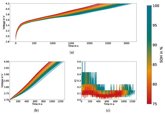
Figure 2.
Full charging curve and extracted features for different SOH over time: (a) Full charging curves as captured during the characterisation tests. (b) Extracted partial charging curves. (c) Derived IC curves.
In order to meet the requirement of a constant input length for the proposed model, the time series data of the selected features are preprocessed by zero-padding to the length of the longest series in the dataset. This length is extended by an additional 10 samples to accommodate for charging curves with slightly longer duration, originated by LIBs with higher initial capacity than those included in the dataset.
Finally, all features will undergo min-max normalisation according to Equation (4)
Here, represents the normalised data, x the original data, and and are the minimum and maximum values of the dataset, respectively. Subsequently, the normalised data are randomly partitioned into three distinct subsets, with 80% of the data used for training, 10% designated for validation, and 10% for testing.
3. Model Structure
Due to its ability to model complex relationships in data and learn hierarchical representations of time series, deep learning has recently emerged as a crucial tool for time series analysis and classification. This work proposes a deep learning model which combines a 1-D CNN and a LSTM neural network to predict the capacity of LIBs based on time series data from partial charging curves. In the proposed topology, the 1-D CNN layer provides the ability to extract additional features from the raw input data, while the LSTM layer is able to capture the long-term dependencies present in the time series data [28].
3.1. 1-Dimensional Convolution Neural Network
A 1-D CNN layer applies a set of learnable filters to the input sequence in order to extract useful features for the given task. Each filter consists of a kernel which slides over the input sequence with a specific stride and width, performing a convolution operation. The output of this convolution is a new sequence, where each element is a weighted sum of the input elements covered by the kernel. For an input sequence x, a filter of length k and a stride of 1, the convolution operation in a discrete form is defined as
where is the i-th element of the output sequence and is the j-th element of the learnable weight of the kernel. After the convolution operation, a non-linear activation function is applied to each element of the output sequence. This introduces non-linearity into the network and helps to capture more complex patterns in the data. In this work, the ReLU function is used as activation.
The number of filters used in a 1-D CNN layer determines the number of output channels, which can be thought of as different feature maps that capture different aspects of the input sequence. Each filter has its own set of learnable weights that are adjusted during training.
3.2. Long Short-Term Memory Neural Network
The LSTM neural network is a type of recurrent neural network (RNN) designed to solve their limitations in learning long-term dependencies in sequential data by addressing the vanishing and exploding gradient problem of traditional RNNs. To do so, LSTM networks incorporate memory into the cell, allowing the selective storage and retrieval of information over long periods of time, hence making them a powerful tool to process time series data.
Figure 3 shows the architecture of a single LSTM cell, where is the input at time t; is the actual cell state, which can be interpreted as the memory of the cell; is the cell state of the previous time step; and is called hidden state, which also acts as the output of the cell. Internally, the cell consists of three gates: the forget gate , the input gate , and the output gate . All internal gates are based on the same equation but with their own trainable weights W and biases b:
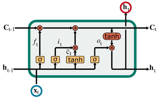
Figure 3.
Schematic structure of an LSTM cell [29].
The results or outputs of these gates decide by multiplication how much information will be forwarded from a specific state. The forget gate controls how much information will be forwarded from the previous to the actual cell state. The input state decides how much of the newly generated memory should be added to the cell state. The new generated memory is defined by
Finally, the output gate controls what information will be forwarded from the actual cell state to the hidden state and thus, to the actual output of the cell. The following formulas define the actual and hidden cell states
where ∗ indicates an element-wise multiplication.
3.3. Applied Topology
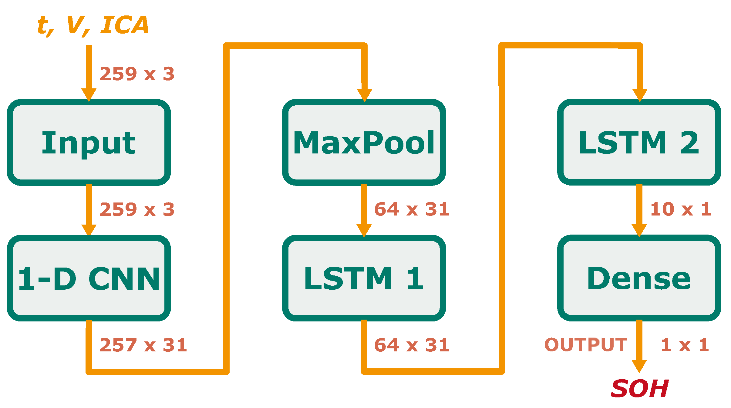
As stated before, this work proposes a combination of a 1-D CNN and LSTM neural networks. Figure 4 depicts a schematic representation of the applied network topology, along with the corresponding input and output dimensionality for each layer.
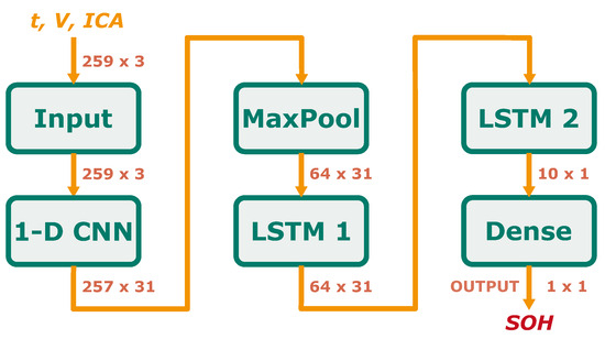
Figure 4.
Schematic representation of the applied network topology, along with the corresponding input and output dimensionality for each layer.
The input features derived from the partial charging curves (time, voltage, and IC) are first processed by a 1D-CNN layer to extract additional features. Subsequently, a one-dimensional maximum pooling layer (1D MaxPooling) is applied to reduce the dimensionality of the resulting multivariate time series through downsampling. The output is then fed into two sequential LSTM layers, followed by a dense layer comprising a single node with a linear activation function, which outputs the estimated SOH.
The extraction of additional features by the 1D-CNN enables a simpler topology for the subsequent LSTM neural network while maintaining high estimation accuracy. This, combined with the downsampling of the multivariate time series processed by the LSTM layers, significantly reduces the storage requirements and computational complexity of the overall network.
3.4. Model Implementation and Training
Keras (version 2.6.0), an open-source deep learning library for Python (version 3.9.7) with TensorFlow (version 2.6.3) as a backend, is used for the implementation and training of the above described neural network. Keras is a high-level API that provides all common deep learning layers, a variety of optimisers, and a model framework for compiling and training. The “Adamax” optimiser with mean-squared error (MSE) as a loss function is applied for training. Regularisation is implemented by a dropout for each LSTM layer to prevent the update of randomly chosen weights after a training step. Dropout decreases the chance of overfitting the network to the training data, thus enhancing the model’s generalisation ability.
Optuna (version 2.10.0), an automated hyperparameter optimisation framework, is utilised to fine-tune a selected set of hyperparameters for both the model and training process. Table 4 lists the hyperparameters which result in the highest estimation accuracy.
Table 4.
Applied hyperparameters.
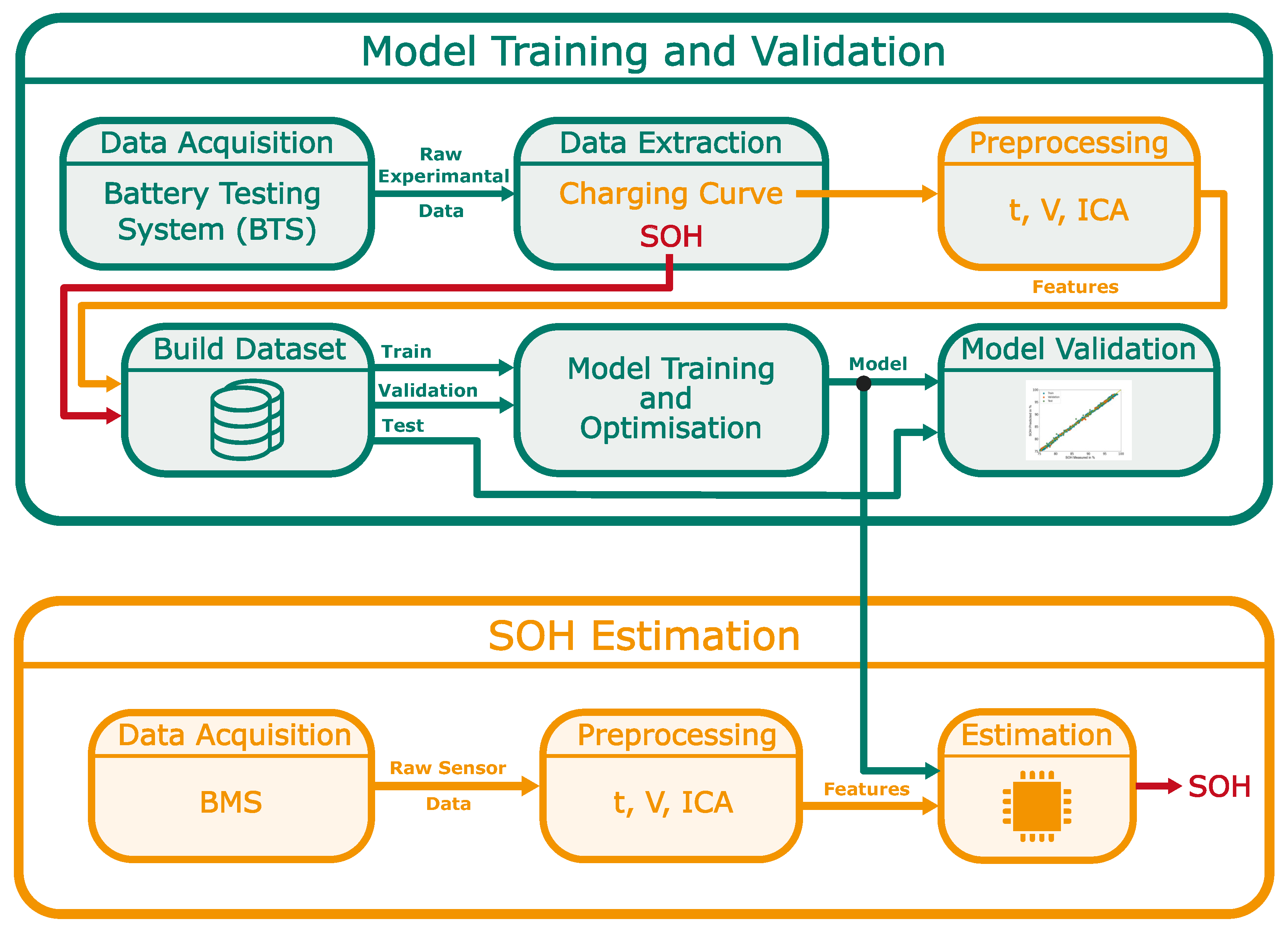
Figure 5 (top) shows the workflow of the model training and validation process, starting with the data acquisition of the raw experimental data supplied by the BTS and subsequent extraction of the charging curves and SOH for each cell and ageing state encompassed in the experiment. The extracted charging curves undergo a preprocessing step where the IC is determined after Equation (2), the partial charging curves (3.7–4.0 V) are extracted, and its features (t, V, IC) undergo normalisation.
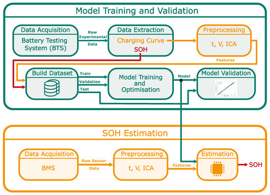
Figure 5.
Schematic representation of the workflow for model training and validation (top) and implementation of the SOH estimation in a real-world application (bottom).
The dataset is then constructed using these preprocessed partial charging curves with their corresponding SOH as labels. The subsequent training and optimisation phase utilises the training subset to train the model and the validation subset to optimise hyperparameters. This optimisation is achieved by evaluating the trained model’s performance on the unseen validation subset and minimising the mean absolute error (MAE) by adjusting the hyperparameters in subsequent training iterations.
Finally, the optimised model is validated by estimating the SOH of the test subset, which remains untouched during both the training and optimisation phases, ensuring an adequate assessment of the robustness and generalisation ability of the model.
Figure 5 (bottom) shows the structure of a possible implementation of the proposed methodology in a real-world application. In this schematic, the BMS captures and archives raw sensor data of voltage and time during the charging process. Subsequently, these raw sensor data undergo preprocessing, mirroring the preprocessing procedures employed during model training. The extracted features are then processed by the trained and validated model deployed either directly on the embedded device integrated within the BMS or on a separate embedded controller especially dedicated to this task.
4. Results and Discussion
In order to assess the quality of the estimations generated by the trained model, three fundamental metrics are employed. The first one is the simple absolute error (AE), which quantifies the absolute difference between estimated and observed values for each individual estimation. The second metric is the mean absolute error (MAE), computed as the arithmetic mean of all AE within a set of estimations. Lastly, the root-mean-square error (RMSE) is utilised, representing the square root of the quadratic mean of the differences between estimated and observed values. MAE and RMSE quantitatively measure the model’s accuracy, whereas the RMSE is more sensitive to outliers. All used metrics indicate better model accuracy with lower values and are defined as follows:
where n is the number of total samples, and the estimated and y the measured SOH in percentage values.
The proposed model is validated under the consideration of three major aspects: first, the determination of the general model performance with respect to the train–validation–test split of the dataset; secondly, its robustness against different ageing scenarios encompassed in the dataset, which is conducted in a cross-validation manner; and the third one focuses on the evaluation of memory usage, computational complexity and actual estimation accuracy of the model by implementing it on a commercially available embedded device.
Additionally, the Bi-LSTM architecture introduced by Li et al. [15] is implemented and trained using the identical dataset, providing a benchmark for comparing the results of the proposed model.
4.1. General Model Performance
The dataset described in Section 2.2 is randomly partitioned into three defined subsets. This train–validation–test split (80%–10%–10%) is used to determine the general model performance. The train subset is used for model training. The validation subset is used to identify potential issues like overfitting during the training process and serves as a target for fine-tuning the hyperparameters. The test subset is not used in the whole training and optimisation process and is most representative of the model’s performance and generalisation ability.
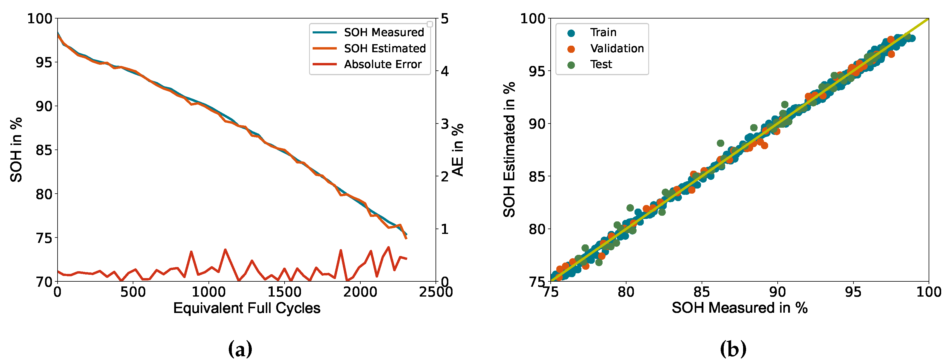
Figure 6a depicts an exemplary representation of the measured and estimated SOH based on the data of cell number 6, along with the absolute error associated with each data point. Notably, the absolute error exhibits a marginal inclination as the SOH decreases but never exceeds the threshold of 1%. Figure 6b shows the deviation between measured and estimated SOH for each datapoint of the dataset separated by the subsets. The yellow line represents an optimal estimation. The deviation shows a homogeneous distribution across all subsets, indicating a high generalisation ability. However, a slight elevation in deviation, accompanied by a rise in the number of outliers, is observed for estimations below SOH = 90%, particularly within the test subset. The corresponding metrics for each subset, together with the results of the Bi-LSTM model proposed by Li et al. [15] are listed in Table 5.
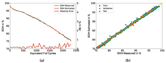
Figure 6.
General model performance of train–validation–test split: (a) Comparison of measured and estimated SOH of cell number 6, including the absolute prediction error. (b) Deviation between measured and estimated SOH for the entire dataset.
Table 5.
Metrics of train–validation–test split.
The archived MAE = 0.473% and RMSE = 0.628% for the test subset underscores the high precision and accuracy of the model in estimating the SOH for unseen data in a real-world application. Relative to the outcomes of the Bi-LSTM, an increase in accuracy can be observed.
4.2. Robustness against Ageing Scenarios
A cross-validation approach over the ageing scenarios described in Section 2.1 is employed to determine the robustness of the model against different ageing mechanisms. For each iteration, the data from a single ageing scenario are designated as the test set, while the data of all remaining scenarios are used for model training. This process is repeated for each ageing scenario listed in Table 2, except for the calendric aged cells (Scenario 8–10). The calendric aged cells are considered to be one scenario due to their similar ageing mechanisms.
The results of the cross-validation are shown in Figure 7, and the corresponding metrics for each scenario are listed in Table 6. In the same manner as for the train–validation–test split, Figure 7a shows the deviation between the measured and estimated SOH for cell number 6, achieving comparable results with a slightly increased absolute error for all estimations but always staying below the threshold of 1%. Figure 7b shows the deviation between measured and estimated SOH of the test set for each iteration (scenario) of the cross-validation. The results demonstrate a similar behaviour as the train–validation–test split, with a homogeneous distribution of deviations across all iterations. This result indicates a high robustness of the model against different ageing scenarios, hence promising an accurate SOH estimation of LIBs under varying usage and environmental conditions in a real-world application.
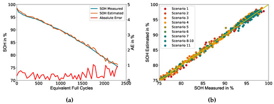
Figure 7.
Model performance of cross-validation over ageing scenarios: (a) Comparison of measured and estimated SOH of cell number 6, including the absolute prediction error. (b) Deviation between measured and estimated SOH for each ageing scenario.
Table 6.
Metrics of cross-validation over scenarios.
4.3. Model Evaluation on Embedded Device
To determine the actual storage occupancy and estimation performance on embedded devices, the trained and optimised model is implemented and deployed on a commercially available ST32-F4 microcontroller manufactured by STMicroelectronics. For implementation and code generation, the ST32Cube IDE (version 1.8.0), in conjunction with the artificial intelligence (AI) extension X-Cube-AI (version 7.1.0), is employed. X-Cube-AI accommodates models constructed with common machine learning libraries such as Keras, PyTorch, or MATLAB and converts them into ST32-optimised c-code libraries.
Table 7 presents the derived storage occupancy and computational complexity after implementation of both the proposed and the Bi-LSTM model introduced by Li et al. [15]. The computational complexity is quantified in terms of multiply–accumulate operations (MACs) and floating-point operations (FLOPs).
Table 7.
Storage occupancy and computational complexity on embedded device.
Both storage requirements and computational complexity are within the capabilities of modern low-budget embedded devices, facilitating the application of the proposed methodology for modern BMS. This is underscored by a significant reduction in storage occupancy and computational complexity compared to the Bi-LSTM model. Particularly noteworthy is the reduction in computational complexity by a factor of 30.
Furthermore, the test subset is evaluated using the implemented model of the proposed methodology on the microcontroller, resulting in slightly higher MAE = 0.475% and RMSE = 0.629%. The decrease in accuracy is likely attributed to the optimisation process for embedded devices conducted by X-Cube-AI, the difference remaining marginal and therefore deemed acceptable.
5. Conclusions
This work proposes a storage- and performance-optimised deep learning model to estimate the capacity-based SOH using time series of raw sensor data from the time, voltage, and IC of partial charging curves under constant current condition. The model combines a 1-D CNN to extract additional features and two sequential LSTM layers to capture long-term dependencies present in the resulting multivariate time series. A 1-D MaxPooling layer is employed to downsample and hence reduce the dimensionality of the multivariate time series generated by the 1D-CNN. The additional feature extraction facilitates a more streamlined topology for the subsequent LSTM layers while maintaining high estimation accuracy. This approach, combined with downsampling, significantly reduces the storage requirements and computational complexity of the overall network.
The successful implementation of the proposed model on a commercially available microcontroller requires 28.54 KB of RAM and 108.7 KB of Flash storage, with a computational complexity of 3.37 × 10⁶ FLOPs. Both the achieved storage occupancy and computational complexity align with the capabilities of modern low-budget embedded devices, making the proposed methodology accessible for commercially produced BMS.
Furthermore, the model has been cross-validated on different ageing scenarios with an average MAE = 0.418% and RMSE = 0.531%, promising accurate SOH estimation of LIBs at varying usage and environmental conditions in a real-world application. A further rise in estimation accuracy is expected for larger datasets used for the training process.
The primary limitation of the proposed methodology lies in its exclusive applicability to scenarios where a controlled charging phase under constant current condition is feasible. In such instances, data acquisition can occur without additional interventions in the battery system’s operation. Additionally, the generation of training data has to be repeated for any additional cell type or applied c-rate, resulting in expensive and time-consuming laboratory work.
Determining if the concept of transfer learning can be applied to reduce these experimental expenses, as well as to prove the suitability of the proposed methodology for other cell chemistries like lithium iron phosphate (LiFePO4), will be the scope of future work.
Author Contributions
Conceptualisation, M.S.; methodology, M.S.; software, M.S.; validation, M.S.; formal analysis, M.S.; investigation, M.S.; resources, J.K.; data curation, M.S.; writing—original draft preparation, M.S.; writing—review and editing, J.K. and M.S.; visualisation, M.S.; supervision, J.K.; project administration, M.S.; funding acquisition, J.K. All authors have read and agreed to the published version of the manuscript.
Funding
This research was funded by the German Federal Ministry for Economic Affairs and Climate Action (BMWK), grant number 16KN086221 (Liobat). The authors are responsible for the content. The work was further supported by the German Research Foundation and the Open Access Publication Fund of TU Berlin.
Data Availability Statement
Data are contained within the article.
Acknowledgments
The author provided the initial authorship and conceptual design of this manuscript, with subsequent refinements and enhancements implemented by AI-based tools such as ChatGPT, DeepL, and Grammarly. It is emphasised that all presented ideas and arguments are the author’s own, and the AI tools were solely employed for linguistic and stylistic improvements. We acknowledge support by the German Research Foundation and the Open Access Publication Fund of TU Berlin.
Conflicts of Interest
The authors declare no conflicts of interest.
Abbreviations
The following abbreviations are used in this manuscript:
| SOH | State of Health |
| LIBs | Lithium-Ion Batteries |
| ICA | Incremental Capacity Analysis |
| IC | Incremental Capacity |
| LSTM | Long Short-Term Memory |
| BMS | Battery Management System |
| MLP | Multilayer Perceptron |
| DNN | Deep Neural Network |
| Bi-LSTM | Bi-directional Long Short-Term Memory |
| 1-D CNN | 1-Dimensional Convolution Neural Network |
| NMC | Lithium-Nickel-Manganese-Cobalt-Oxide |
| C | Carbon |
| DOD | Depth of Discharge |
| SOC | State of Charge |
| FUDS | Federal Urban Driving Schedule |
| BTS | Battery Testing System |
| OCV | Open Circuit Voltage |
| CC | Constant Current |
| RNN | Recurrent Neural Network |
| 1-D MaxPooling | 1-Dimensional Maximum Pooling |
| AE | Absolute Error |
| MAE | Mean Absolute Error |
| RMSE | Root Mean Square Error |
| AI | Artificial Intelligence |
| MACs | Multiply–Accumulate Operations |
| FLOPs | Floating Point Operations |
References
- Killer, M.; Farrokhseresht, M.; Paterakis, N.G. Implementation of large-scale Li-ion battery energy storage systems within the EMEA region. Appl. Energy 2020, 260, 114166. [Google Scholar] [CrossRef]
- Masias, A.; Marcicki, J.; Paxton, W. Opportunities and Challenges of Lithium Ion Batteries in Automotive Applications. ACS Energy Lett. 2021, 6, 621–630. [Google Scholar] [CrossRef]
- Vetter, J.; Novák, P.; Wagner, M.R.; Veit, C.; Möller, K.C.; Besenhard, J.O.; Winter, M.; Wohlfahrt-Mehrens, M.; Vogler, C.; Hammouche, A. Ageing mechanisms in lithium-ion batteries. J. Power Sources 2005, 147, 269–281. [Google Scholar] [CrossRef]
- Li, Y.; Abdel-Monem, M.; Gopalakrishnan, R.; Berecibar, M.; Nanini-Maury, E.; Omar, N.; van den Bossche, P.; van Mierlo, J. A quick on-line state of health estimation method for Li-ion battery with incremental capacity curves processed by Gaussian filter. J. Power Sources 2018, 373, 40–53. [Google Scholar] [CrossRef]
- Riviere, E.; Sari, A.; Venet, P.; Meniere, F.; Bultel, Y. Innovative Incremental Capacity Analysis Implementation for C/LiFePO4 Cell State-of-Health Estimation in Electrical Vehicles. Batteries 2019, 5, 37. [Google Scholar] [CrossRef]
- Gantenbein, S.; Schönleber, M.; Weiss, M.; Ivers-Tiffée, E. Capacity Fade in Lithium-Ion Batteries and Cyclic Aging over Various State-of-Charge Ranges. Sustainability 2019, 11, 6697. [Google Scholar] [CrossRef]
- Andre, D.; Meiler, M.; Steiner, K.; Wimmer, C.; Soczka-Guth, T.; Sauer, D.U. Characterization of high-power lithium-ion batteries by electrochemical impedance spectroscopy. I. Experimental investigation. J. Power Sources 2011, 12, 5334–5341. [Google Scholar] [CrossRef]
- Zhang, Y.; Tang, Q.; Zhang, Y.; Wang, J.; Stimming, U.; Lee, A.A. Identifying degradation patterns of lithium ion batteries from impedance spectroscopy using machine learning. Nat. Commun. 2020, 11, 1706. [Google Scholar] [CrossRef] [PubMed]
- Bi, J.; Zhang, T.; Yu, H.; Kang, Y. State-of-health estimation of lithium-ion battery packs in electric vehicles based on genetic resampling particle filter. Appl. Energy 2016, 182, 558–568. [Google Scholar] [CrossRef]
- Zou, Y.; Hu, X.; Ma, H.; Li, S.E. Combined State of Charge and State of Health estimation over lithium-ion battery cell cycle lifespan for electric vehicles. J. Power Sources 2015, 273, 793–803. [Google Scholar] [CrossRef]
- Bartlett, A.; Marcicki, J.; Onori, S.; Rizzoni, G.; Yang, X.G.; Miller, T. Electrochemical Model-Based State of Charge and Capacity Estimation for a Composite Electrode Lithium-Ion Battery. IEEE Trans. Control. Syst. Technol. 2015, 24, 384–399. [Google Scholar] [CrossRef]
- Zheng, L.; Zhang, L.; Zhu, J.; Wang, G.; Jiang, J. Co-estimation of state-of-charge, capacity and resistance for lithium-ion batteries based on a high-fidelity electrochemical model. Appl. Energy 2016, 180, 424–434. [Google Scholar] [CrossRef]
- Roman, D.; Saxena, S.; Robu, V.; Pecht, M.; Flynn, D. Machine learning pipeline for battery state-of-health estimation. Nat. Mach. Intell. 2021, 3, 447–456. [Google Scholar] [CrossRef]
- Wei, Z.; Ruan, H.; Li, Y.; Li, J.; Zhang, C.; He, H. Multistage State of Health Estimation of Lithium-Ion Battery with High Tolerance to Heavily Partial Charging. IEEE Trans. Power Electron. 2022, 37, 7432–7442. [Google Scholar] [CrossRef]
- Li, W.; Sengupta, N.; Dechent, P.; Howey, D.; Annaswamy, A.; Sauer, D.U. Online capacity estimation of lithium-ion batteries with deep long short-term memory networks. J. Power Sources 2021, 482, 228863. [Google Scholar] [CrossRef]
- Zhao, J.; Zhu, Y.; Zhang, B.; Liu, M.; Wang, J.; Liu, C.; Zhang, Y. Method of Predicting SOH and RUL of Lithium-Ion Battery Based on the Combination of LSTM and GPR. Sustainability 2022, 14, 11865. [Google Scholar] [CrossRef]
- Richardson, R.R.; Birkl, C.R.; Osborne, M.A.; Howey, D.A. Gaussian Process Regression for In Situ Capacity Estimation of Lithium-Ion Batteries. IEEE Trans. Ind. Inform. 2019, 15, 127–138. [Google Scholar] [CrossRef]
- Guo, Y.; Huang, K.; Hu, X. A state-of-health estimation method of lithium-ion batteries based on multi-feature extracted from constant current charging curve. J. Energy Storage 2021, 36, 102372. [Google Scholar] [CrossRef]
- Klass, V.; Behm, M.; Lindbergh, G. A support vector machine-based state-of-health estimation method for lithium-ion batteries under electric vehicle operation. J. Power Sources 2014, 270, 262–272. [Google Scholar] [CrossRef]
- Liu, K.; Kang, L.; Xie, D. Online State of Health Estimation of Lithium-Ion Batteries Based on Charging Process and Long Short-Term Memory Recurrent Neural Network. Batteries 2023, 9, 94. [Google Scholar] [CrossRef]
- Fan, Y.; Xiao, F.; Li, C.; Yang, G.; Tang, X. A novel deep learning framework for state of health estimation of lithium-ion battery. J. Energy Storage 2020, 32, 101741. [Google Scholar] [CrossRef]
- Rzepka, F.; Hematty, P.; Schmitz, M.; Kowal, J. Neural Network Architecture for Determining the Aging of Stationary Storage Systems in Smart Grids. Energies 2023, 16, 6103. [Google Scholar] [CrossRef]
- Zhang, C.; Luo, L.; Yang, Z.; Zhao, S.; He, Y.; Wang, X.; Wang, H. Battery SOH estimation method based on gradual decreasing current, double correlation analysis and GRU. Green Energy Intell. Transp. 2023, 2, 100108. [Google Scholar] [CrossRef]
- Zhang, C.; Zhao, S.; Yang, Z.; Chen, Y. A reliable data-driven state-of-health estimation model for lithium-ion batteries in electric vehicles. Front. Energy Res. 2022, 10, 1013800. [Google Scholar] [CrossRef]
- Zheng, Y.; Wang, J.; Qin, C.; Lu, L.; Han, X.; Ouyang, M. A novel capacity estimation method based on charging curve sections for lithium-ion batteries in electric vehicles. Energy 2019, 185, 361–371. [Google Scholar] [CrossRef]
- BEXEL. Specifications Li-ion INR18650 2600 SP01(Lithium Battery); BEXEL: Seoul, Republic of Korea, 2018. [Google Scholar]
- Han, X.; Ouyang, M.; Lu, L.; Li, J.; Zheng, Y.; Li, Z. A comparative study of commercial lithium ion battery cycle life in electrical vehicle: Aging mechanism identification. J. Power Sources 2014, 251, 38–54. [Google Scholar] [CrossRef]
- Ismail Fawaz, H.; Forestier, G.; Weber, J.; Idoumghar, L.; Muller, P.A. Deep learning for time series classification: A review. Data Min. Knowl. Discov. 2019, 33, 917–963. [Google Scholar] [CrossRef]
- Colah, C. Understanding LSTM Networks. 2015. Available online: https://colah.github.io/posts/2015-08-Understanding-LSTMs/ (accessed on 24 January 2024).


Disclaimer/Publisher’s Note: The statements, opinions and data contained in all publications are solely those of the individual author(s) and contributor(s) and not of MDPI and/or the editor(s). MDPI and/or the editor(s) disclaim responsibility for any injury to people or property resulting from any ideas, methods, instructions or products referred to in the content. |
© 2024 by the authors. Licensee MDPI, Basel, Switzerland. This article is an open access article distributed under the terms and conditions of the Creative Commons Attribution (CC BY) license (https://creativecommons.org/licenses/by/4.0/).