A Physics–Guided Machine Learning Approach for Capacity Fading Mechanism Detection and Fading Rate Prediction Using Early Cycle Data

Abstract

Lithium–ion battery development necessitates predicting capacity fading using early cycle data to minimize testing time and costs. This study introduces a hybrid physics–guided data–driven approach to address this challenge by accurately determining the dominant fading mechanism and predicting the average capacity fading rate. Physics–guided features, derived from the electrochemical properties and behaviors within the battery, are extracted from the first five cycles to provide meaningful, interpretable, and predictive data. Unlike previous models that rely on a single regression approach, our method utilizes two separate regression models tailored to the identified dominant fading mechanisms. Our model achieves 95.6% accuracy in determining the dominant fading mechanism using data from the second cycle and a mean absolute percentage error of 17.09% in predicting lifetime capacity fade from the first five cycles. This represents a substantial improvement over state–of–the–art models, which have an error rate approximately three times higher. This study underscores the significance of physics–guided data characterization and the necessity of identifying the primary fading mechanism prior to predicting the capacity fading rate in lithium–ion batteries.

1. Introduction

Lithium–ion batteries (LiBs) have become a key element in the transition to renewable energy due to their high specific energy and power density, falling costs, long life, low self–discharge rate, and lack of memory effect [1]. Many battery studies have focused on material synthesis, electrolyte development, and cell engineering. These efforts have advanced battery performance by controlling its design and manufacturing. A capacity degradation study is usually conducted to evaluate the performance of such a development. However, the degradation of LiBs is a lengthy process that poses a challenge to their development and deployment. Given the widespread use of LiBs, early prediction of their degradation behavior has become increasingly important. However, this task is challenging due to their nonlinear degradation over cycles, wide variability, and the necessity to meet specific operating conditions.

Model–based methods have been developed to predict the degradation behavior and address the early prediction problem. Model–based methods utilize models that describe batteries’ internal chemical reactions and degradation mechanisms to predict the cycle life by considering the changes in specific mechanisms. These methods range from semi–empirical models to electrochemical models [2,3,4]. A challenge for these methods is parameterization, often addressed by parameter estimation algorithms such as the Kalman filter [5], and Particle filter [6]. Although these model–based methods have achieved some predictive success, developing comprehensive models for full cells to predict cycle life and determining model parameters for early cycle life prediction with limited data remains challenging due to the variety of degradation modes in a cell, which are coupled with mechanical and thermal heterogeneities [7].

Due to the complexity of utilizing model–based methods, statistical and machine learning methods have gained popularity for predicting battery lifetime from early cycle data thanks to recent advancements in algorithms, computational power, and data accessibility. Severson et al. developed a linear model–elastic net—that can accurately predict the battery cycle life with features extracted from the first 100 cycles [8]. By utilizing a more advanced regression model and undergoing sophisticated feature selection and engineering, Attia et al. achieved comparable or improved accuracy on the same dataset [9]. Gaussian process regression (GPR) has also become very popular for estimating battery degradation using early cycle data. Li et al. proposed a GPR model to predict the battery capacity and battery lifetime with features extracted from the dQ/dV curves from the first 30 cycles [10]. Richardson et al. proposed the integration of a conventional covariance–function–based GPR model with an explicit mean function, which can provide prior knowledge for lifetime prediction [11]. A support vector machine (SVM) has also been applied to estimate the lifetime [7,12,13]. Neural networks, with their good performance in solving nonlinear dynamic problems, have been applied widely in predicting degradation behavior. With features extracted and transformed from the capacity, voltage, current, and internal resistance recorded in the early cycle, Zhang et al. then employed a general regression neural network to predict the battery lifetime [14]. Xu et al. selected features from the discharge process and used a stacked denoising autoencoder to predict the battery lifetime [15]. Moreover, with a powerful deep neural network, given capacity, voltage, current, and temperature from the first cycle, the author was able to predict the battery life [16]. Yao et al. use autoencoder to extract features from multiple cycle follows with an elastic model to predict the battery lifetime given early cycle data [17]. However, neural networks, especially deep neural networks, are black box models and lack physics insight, leading to poor performance when extrapolating to regions not covered by the training data. Hybrid models, in which the core physics of the battery is combined with a data–driven model, have the potential to tackle such problems. Hybrid models are fast and have a low computational burden once trained by taking advantage of a physics–based model, including battery physics. Moreover, thanks to the core physics, these hybrid models’ interpretability can help generalize the dataset and develop a physics–guided model [18]. Thelen et al. integrated experimental early degradation data with simulation data generated by a physics–based model to predict degradation behavior [19]. Instead of using the physics–based model to generate training data, by incorporating the physics constraint with the neural network’s loss function, Najera–Flores et al. outperformed the model–based method and a machine learning method in battery remaining useful life prediction [20]. Furthermore, by combining a physics–based calendar and cycle aging model with a long short–term memory layer, Shi et al. proposed physics–informed machine learning for remaining useful life prediction [21]. Despite these pioneering works, in these previous studies, even though the cycle data are generated with varying operating conditions, which cover many degradation patterns, these studies attempted to propose a universal prediction model to perform a lifetime prediction, which may affect the model’s predictability due to the underlying different fading mechanism. Some work has been conducted to address this issue. Severson et al. [8], Deng et al. [22], and Jiang et al. [23] proposed methods that can classify batteries into different groups with different capacity fading rates. However, these classification methods are data–driven and lack a physical explanation of the degradation patterns behind them. In contrast, recent works have correlated selected features and degradation modes with electrochemical explanations [24,25]. For example, Chen et al. demonstrated that the end–of–charge voltage is one of the strong indicators that distinguishes two major aging mechanisms: solid–electrolyte interphase (SEI) growth and Li plating [24]. With an understanding of different fading mechanisms, physics–guided electrochemical features can be extracted and create an explainable classification algorithm along with high accuracy. However, these studies lack predictive capability and fail to forecast the rate of degradation.

In this work, we propose a hybrid physics–guided and data–driven model to address a critical problem during battery operation: predicting capacity fading with early–stage data. Physics–guided features, based on a thorough understanding of battery physics, allow us to effectively identify degradation modes and accurately predict degradation behavior using early cycle data. These physics–guided features are integrated into our model to accurately reflect the physical and chemical states of the battery, thereby enhancing its predictive power and reliability. Moreover, with the understanding of battery physics, a physics–guided framework first determines the dominant fading mechanism of the battery through classification and then applies regression models tailored to each specific fading mechanism. Utilizing these features and the proposed framework, we develop a machine –learning approach that can predict the capacity fade rate with high accuracy. This model can significantly expedite the optimization of the battery charging protocol using early cycle data and reduce the test time for battery cycle tests, a common practice in battery development and deployment.

2. Data Generation

Commercial Li–ion coin cells (LIR2025H produced by EEMB Battery) with nickel manganese cobalt oxide (NMC) cathodes and graphite anodes are cycled on a Landt CT3001A battery test system to generate data for model development at different temperatures (Supplementary Materials Table S1). In each cycle, the battery is first charged by a constant–current constant–voltage (CCCV) method, i.e., the battery is charged at a pre–defined current until its voltage reaches a pre–defined cut–off voltage. Then, the charging voltage is fixed at this cut–off voltage until the charging current drops below C/50. After charging, the battery rests for 3600 s or 600 s and is then discharged to a cut–off voltage of 2.75 V at a constant current (CC), followed by a 600 s rest. Therefore, each cycle consists of four steps: CCCV charge, rest, CC discharge, and rest (Figure 1a). A total of 45 batteries are tested, and they are charged under different conditions during the CCCV charging with differing charging current and cut–off voltage but are discharged at the same rate (C/5) (Supplementary Materials Table S1). Two data streams from the raw cycle data are used for feature engineering and model development:

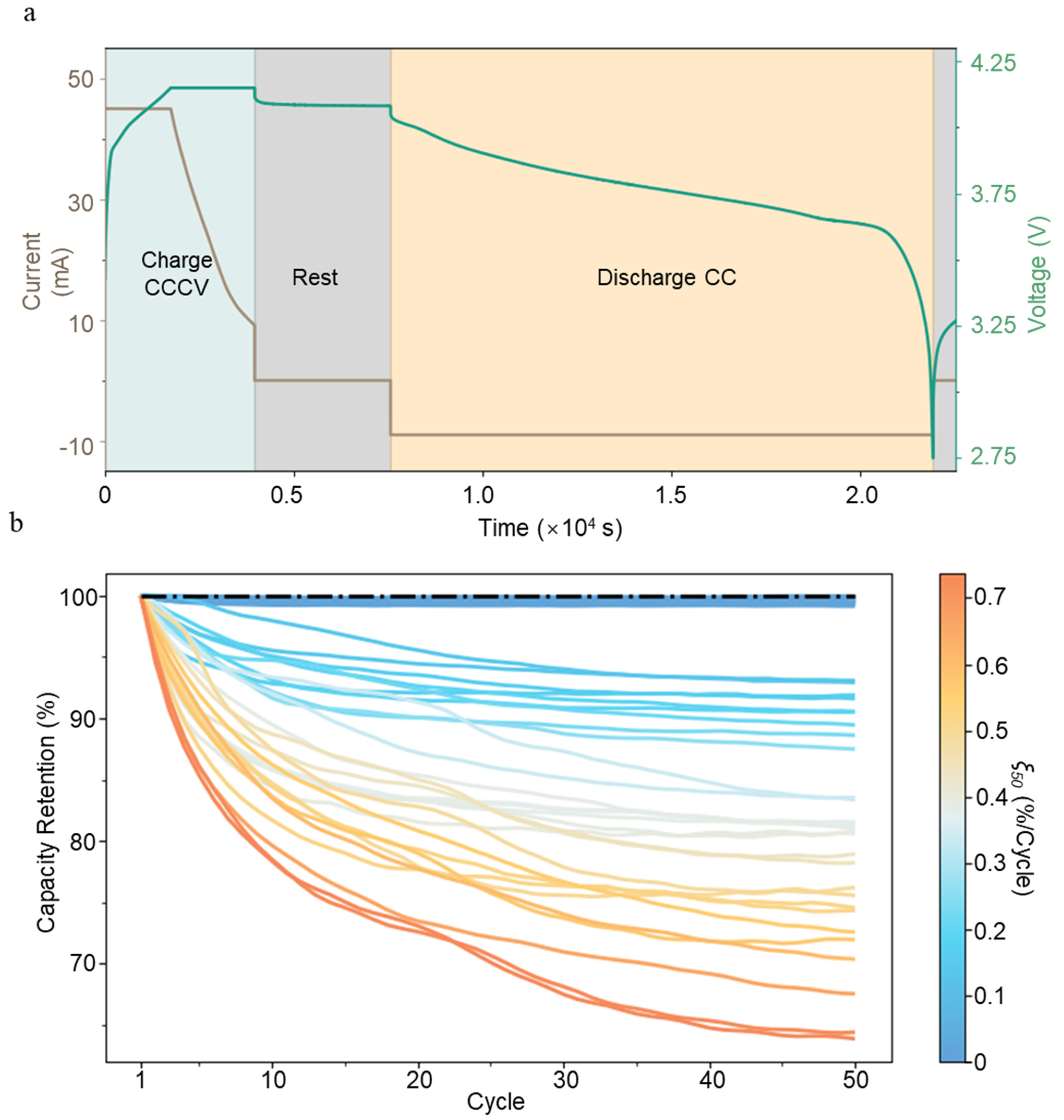
• The first data stream contains the voltage of the battery, V(t), during cycling (Figure 1a). The side reactions inside the battery, lithium deposits on the graphite anode, and the growth of the SEI cause the battery capacity to decay. Their effects are manifested in the shape of the V(t) curve. Therefore, the features from the V(t) and I(t) curves contain physical information about side reactions. For example, incremental capacity analysis can be conducted, and features such as peak location and peak area can be used to identify the fading mode [26]. Note that I(t) is predetermined as the input for battery cycling for constant current charge and discharge.
• The second data stream contains the discharging capacity C(N) and Faraday efficiency η(N) for each cycle (Figure 1b). N refers to the battery cycle number. C(N) is used to calculate the rate of capacity fading. The normalized capacity of each battery is shown in Figure 1b. Based on this data stream, the average capacity fading rate at the Nth cycle, ${\xi }_N$, is calculated as follows:

$${\xi }_N={\displaystyle \frac{C_1-C_N}{\left(N-1\right)C_1}}\times 100\%$$

(1)

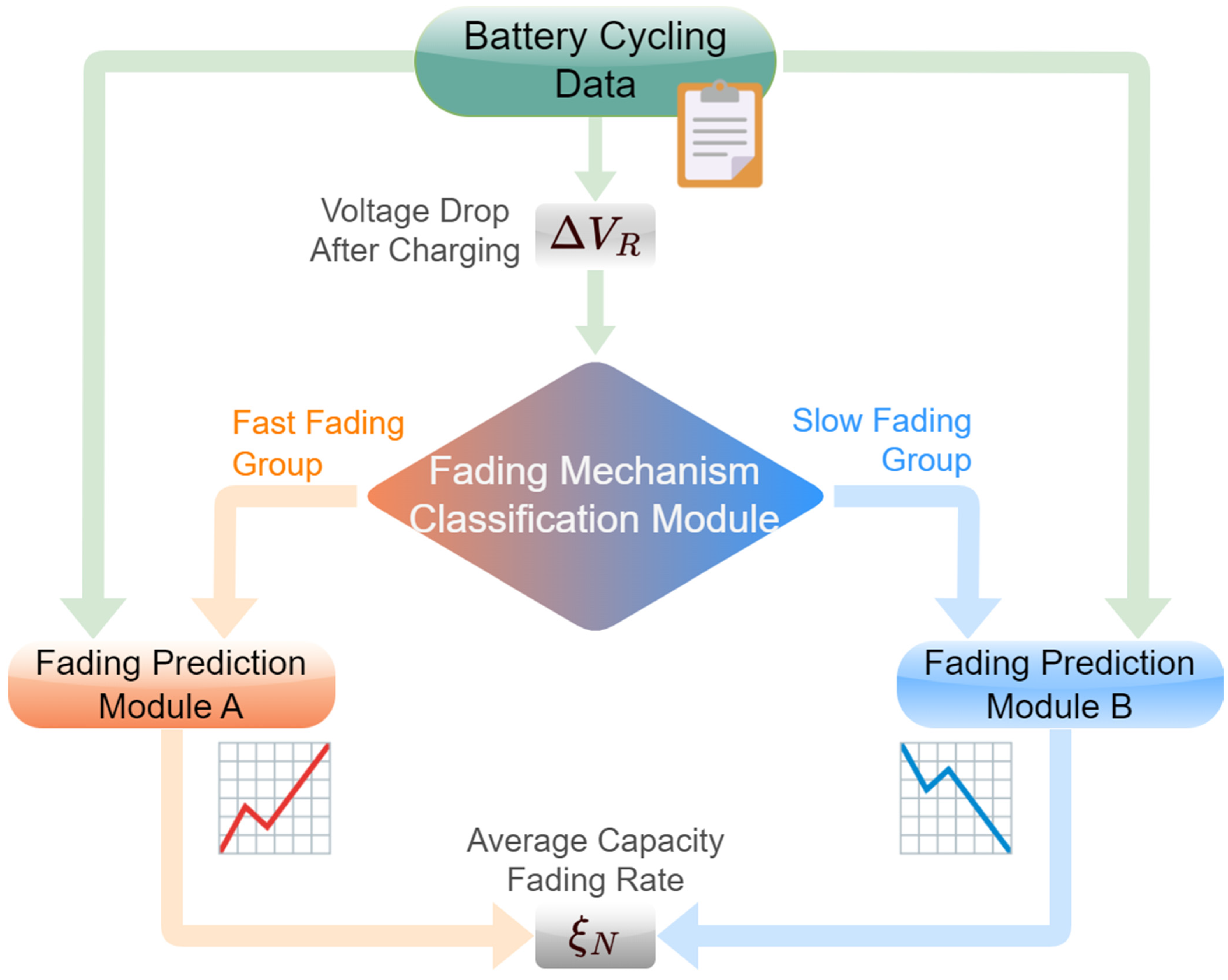
3. Model Framework

The model consists of two modules: (1) the fading mechanism classification module, which classifies batteries charged under different protocols into two groups based on the dominant capacity fading mechanism, and (2) the average capacity fading rate prediction module, which separately predicts the average capacity fading rate of the batteries in each group (Figure 2). Li–ion batteries lose usable capacity during charge/discharge cycling, mainly due to the loss of active lithium ions. During charging/discharging, the active lithium ions carry charges and shuttle back and forth between the cathode/anode host, where side reactions occur. The loss of active lithium ions can be attributed to serval mechanisms: (1) SEI growth on graphite particles and (2) irreversible Li plating are the two most common reasons. SEI growth dominates under moderate conditions, and Li plating usually occurs at high charging rates. The current physical understanding does not provide an explicit boundary to distinguish the primary capacity fading mechanism for batteries cycled under different conditions. We show that such a boundary can be drawn with an unsupervised machine learning algorithm based on a feature that carries the physical information of the Li plating mechanism (fading mechanism classification module). With this algorithm, batteries will be classified into two groups: the Slow Fading Group, corresponding to batteries whose capacity fading is mainly governed by SEI growth, and the Fast Fading Group, corresponding to batteries whose capacity fading is dominated by Li plating. Two separate regression algorithms are built using features containing the physical information of the corresponding fading mechanism, which are used to predict the capacity fading rate for batteries in each group.

4. Machine–Learning Model Development

4.1. K–Mean Clustering

Given an unlabeled dataset, the aim of K–means clustering is to partition the observation into k clusters, which minimizes the within–cluster sum of squares, such as variance. Given a set of datapoints, $X=\left\{x_1,x_2,x_3,\dots ,x_n\right\}$, K–means clustering aims to group the n datapoint into k sets $S=\left\{S_1,S_2,S_3,\dots ,S_k\right\}$. The objective can be expressed as

$$\underset{S}{\arg \min }{\displaystyle \sum _{i=1}^k{\displaystyle \sum _{x\in S_i}{‖x-{\mu }_i‖}^2}}$$

(2)

where ${\mu }_i$ is the centroid of cluster i. The k value, which is the number of the cluster, will affect the K–means algorithm and needs to be specified before conducting any clustering analysis [27]. As mentioned before, depending on the operating conditions, the LiBs are subjected to different dominant degradation mechanisms. In this study, k is set to 2, inspired by the two dominant fading mechanisms: SEI growth and Li plating.

4.2. Linear Support Vector Regression

SVM is initially proposed by Cortes et al. to solve classification problems [28]. Drucker et al. adopted the principle of SVM and proposed a support vector regressor (SVR) [29]. SVMs have a solid theoretical foundation rooted in statistical learning theory and require only a small number of samples for training [30]. However, like any other model, the description and understanding of the data, including the number of dimensions, are crucial for model performance. Given a training dataset $D=\left\{\left(x_i,y_i\right),i=1,2,\dots ,n\right\}\left(x_i\in X=R^d,y_i\in Y=R\right)$, the linear SVR method maps the training dataset from the low–dimensional mapping space to the high–dimensional space through nonlinear mapping by solving the following primal problem:

$$\underset{w,b}{\min }\left({\displaystyle \frac{1}{2}}{w}^{T}w+C{\displaystyle \sum _{i=1}^n\max \left(0,\left|y_i-\left(w^T\varphi \left(x_i\right)+b\right)\right|-ϵ\right)}\right)$$

(3)

where $w\in R^d$, $ϵ$ is introduced to control sensitivity to loss which ignores errors less than $ϵ$, and C is a regularization term. The dual problem is formulated as

$$\begin{array}{l}\underset{a,a^{\ast }}{{\displaystyle \max }}\left({\displaystyle \sum _{i=1}^n\left(a_i-a_i^{\ast }\right)y_i}-{\displaystyle \sum _{i=1}^n\left(a_i+a_i^{\ast }\right)ϵ}-{\displaystyle \frac{1}{2}}{\displaystyle \sum _{i=1}^n{\displaystyle \sum _{j=1}^n{\left(a_i-a_i^{\ast }\right)}^{T}Q\left(a_j-a_j^{\ast }\right)}}\right)\\ s.t.\left\{\begin{array}{c}{\displaystyle \sum _{i=1}^n\left(a_i-a_i^{\ast }\right)=0}\\ 0\le a_i,a_i^{\ast }\le C,\forall i\end{array}\right.\end{array}$$

(4)

where $Q\in R^{n\times n}$ and the value within the matrix is calculated as $Q_{ij}=\varphi {\left(x_i\right)}^T\varphi \left(x_j\right)$. To evaluate the performance, the predicted average capacity fading rate should be compared to the actual fading rate. In this study, two performance metrics are considered: root mean square error (RMSE) and mean absolute percent error (MAPE), which are defined as

$$\mathrm{RMSE}=\sqrt{{\displaystyle \frac{1}{n}}{\displaystyle \sum _{i=1}^n{\left(y_i-{\widehat{y}}_i\right)}^2}}$$

(5)

$$\mathrm{MAPE}={\displaystyle \frac{1}{n}}{\displaystyle \sum _{i=1}^n\frac{\left|y_i-{\widehat{y}}_i\right|}{y_i}}\times 100\%$$

(6)

5. Results

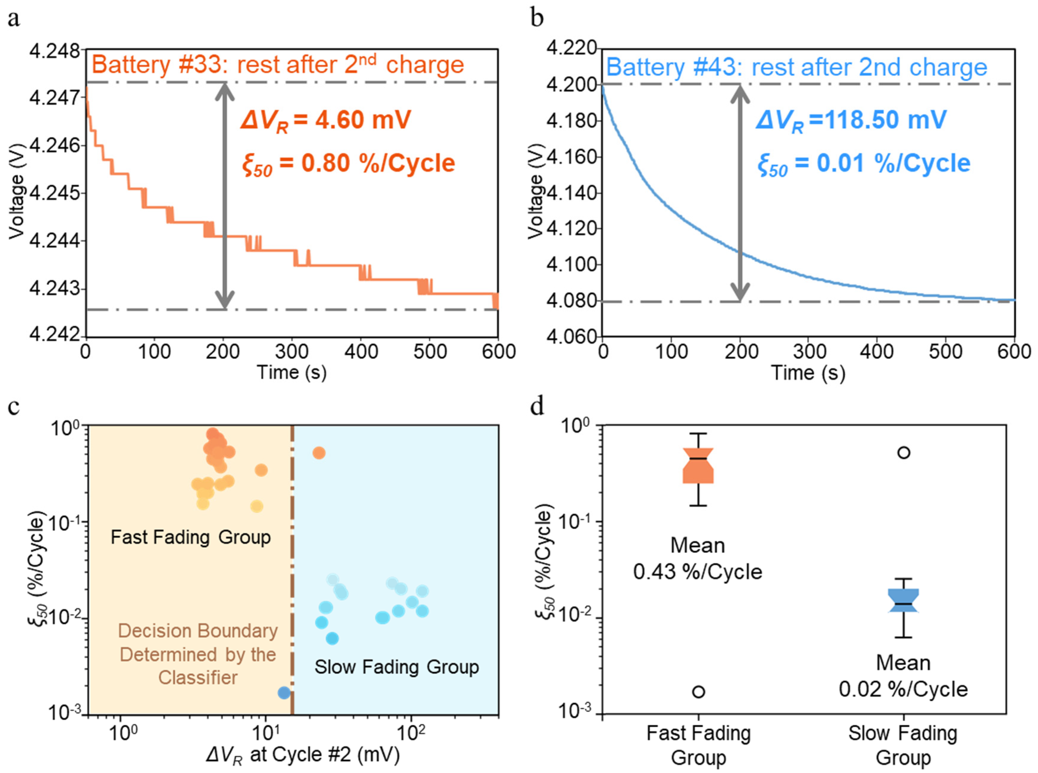
5.1. Fading Mechanism Classification

To develop a physics–guided machine learning algorithm for classifying batteries based on their primary capacity fading mechanism, the feature needs to contain the physical information of the fading mechanism. For Li–ion batteries, two mechanisms, SEI growth, and Li plating, contribute to the loss of active lithium ions and cause capacity fading. During charging, lithium ions are extracted from the oxide cathode, and meanwhile, lithium ions in the electrolyte near the anode are intercalated into the graphite anode. Under slow charging conditions (typically < C/3), the battery’s capacity fading is mainly governed by the slow growth of SEI on the graphite anode, which gradually consumes the active lithium–ion inventory in the battery [31]. However, under fast charging conditions, a different capacity fading mechanism kicks in. When charged at a high rate, the insertion of Li into the graphite particles can outpace the diffusion of Li in graphite and lead to the saturation of the graphite particles on the surface [32]. As a result, Li plating occurs on the particles. During battery rest, a portion of the plated Li can still intercalate into the graphite, but some lose electrical contact with the graphite particles and become “dead”. Therefore, Li plating consumes the Li inventory much faster than SEI growth, resulting in faster capacity fading.

Among these two data streams, V(t) is a time series that reflects the battery’s changing internal environment during cycling. More specifically, V(t) is determined by the electrochemical potential of the electrode and the dynamics of various physical and chemical processes inside the battery. During the resting stage after charging, the change in voltage reflects the elimination of the Li insertion/extraction reaction at the interface, transportation of ions to balance the concentration inhomogeneity in the electrolyte, and diffusion of lithium ions to balance the chemical potential inhomogeneity in the electrode materials. When the battery enters the resting stage from the charging stage, the voltage profile usually consists of a sudden drop, which corresponds to the elimination of the reaction and ohmic overpotentials, followed by a gradual decay, which corresponds to the removal of the concentration or chemical potential gradient in the electrolyte and the electrode material (both oxide cathode and graphite anode). Given sufficient rest, the voltage reaches a plateau that corresponds to the equilibrium state of the battery. The voltage of the battery can be described by an electrochemical equation with F as Faraday’s constant (Equation (7)) (see Supplementary Materials Note S2 for the derivation), in which the four terms correspond to the difference in surface chemical potential between the oxide cathode and the graphite anode, the concentration overpotential in the electrolyte, the ohmic overpotential in the electrolyte, and the reaction overpotential at the electrode/electrolyte interface. The last two terms vanish instantly once the battery enters the resting stage, and the second term tends toward zero as the electrolyte concentration gradient disappears. Without plated Li, the first term tends to reach the equilibrium voltage of the battery. In the graphite particles, the surface chemical potential (μ_d^g) decreases because the diffusion of the inserted lithium ions toward the particle’s interior reduces the lithium–ion concentration on the particle surface. However, if Li plates on graphite, the plated Li will react with graphite during the resting stage, so the surface lithium–ion concentration will remain constant until this reaction finishes. As a result, μ_d^g remains invariant, and the voltage drop only comes from the oxide, which will be reduced, compared to the case without Li plating.

$$V_{Bat}=-{\displaystyle \frac{{\mu }_d^o-{\mu }_d^g}{F}}+{\displaystyle \frac{{\mu }_{L{i}^{+}}^o-{\mu }_{L{i}^{+}}^g}{F}}+\left({\varphi }_l^o-{\varphi }_l^g\right)+\left({\eta }^o-{\eta }^g\right)$$

(7)

$$\Delta V_R=V_0-V_{600}$$

(8)

Based on the above discussion, the voltage drops during the resting stage, ∆V_R, which is the voltage change within the first 600 s after CCCV charging, should effectively represent the capacity fading mechanism (Equation (8)). To confirm this, two batteries with drastically different capacity fade rates are chosen, and their V(t) profiles during the resting stage are compared in Figure 3. The fast capacity fading of battery 33 is due to Li plating, whereas the slow capacity fading of battery 43 is due to SEI growth (Supplementary Materials Note S4). Evidently, their V(t) profiles are distinct. Battery 43 (no Li plating) shows a smooth V(t) curve with ∆V_R = 118.5 mV, whereas battery 33 (with Li plating) shows a zig–zag V(t) profile with ∆V_R = 4.6 mV, which is two orders of magnitude lower. The zig–zag shape of the V(t) profile is due to the limited number of data points being sampled in the experiment for a small ∆V_R. As discussed above, such a small voltage drop is because graphite particles with plated lithium fail to relax (reducing their surface lithium–ion concentration) during the resting stage, which occurs because the plated Li keeps intercalating with graphite particles and maintains its surface potential. A similar result has been observed in the experiment, where the voltage changes slowly during the rest period for graphite particles with plated lithium [32]. In contrast, for battery 43, without the intercalation of plated Li, the surface Li–ion concentration will gradually decrease, reducing the Li–ion concentration gradient within the graphite particle. Consequently, the additional relaxation in the graphite particle results in a much higher ∆V_R compared to the battery 33. A similar behavior can be observed when comparing their V(t) profiles in other cycles (Supplementary Material Figure S3). Additionally, consistent differences are evident when comparing batteries with slow capacity fading (Supplementary Material Figure S5) to those with fast capacity fading (Supplementary Material Figure S4).

The above examples suggest that ∆V_R could be a good feature for constructing a classification machine learning algorithm that can group batteries based on the capacity fading mechanism. Moreover, by measuring the voltage drop during the resting stage after constant voltage charging within a cycle, rather than the voltage value itself at a certain time, we can capture the process of relaxation and reduce the impact of different constant charging voltages. This approach allows us to eliminate the influence of different charging conditions and focus on ∆V_R to understand the cell’s potential relaxation during the resting stage. To develop such an algorithm, ∆V_R of all the batteries at the 2nd cycle is computed and plotted on a log scale (Figure 3c). Visually, all data points fall into two groups: one located in the bottom–left region of the plot and another located in the top–right– area of the plot. Given a total of 45 cells, a boundary can be drawn by unsupervised machine learning using a K–means clustering algorithm (Figure 3c), which divides all batteries into two groups: Fast Fading Group (orange region) showing a ∆V_R < 15.6 mV and Slow Fading Group (blue region) showing a ∆V_R > 15.6 mV. To examine if this boundary can distinguish between batteries with different primary fading mechanisms, the capacity fade rate (${\xi }_{50})$ of each group is plotted in a boxplot on a log scale (Figure 3d). Clearly, batteries classified into the Fast Fading Group (median = 0.45%/Cycle, mean = 0.43%/Cycle) have significantly higher capacity fading rates than batteries in the Slow Fading Group (median = 0.01%/Cycle, mean = 0.02%/Cycle). By treating outliers as incorrectly classified, given the second cycle data, the classification achieves a 4.3% error rate. A similar classification can be achieved using only the V(t) data from the other early cycles (Supplementary Materials Figure S6), indicating the reliability of the ∆V_R feature. As the batteries cycle, for batteries with Li plating as the dominant fading mechanism, the usable capacity decreases quickly, resulting in a higher real C–rate, which makes the lithium plating servers. Therefore, the classification result improves with the ∆V_R collected from a later cycle (Supplementary Materials Figure S6). These results demonstrate that using ∆V_R as a single feature, an unsupervised machine learning module can accurately cluster batteries into two groups: a Fast Fading Group with Li plating as the main fading mechanism and a Slow Fading Group with SEI growth as the main fading mechanism. Being able to identify the main capacity fading mechanism is a critical step in realizing the accurate prediction of battery capacity during cycling for two reasons: (1) it enables feature selection based on the fading mechanism without having to resort to the time–consuming feature engineering process in a typical machine learning model development; (2) by carefully examining the fading mechanism, features containing the most relevant information can be identified, which can increase the prediction accuracy of the model. In the next section, we discuss how we choose such physics–guided features to construct a machine learning algorithm to predict battery capacity fading based on the dominant fading mechanism.

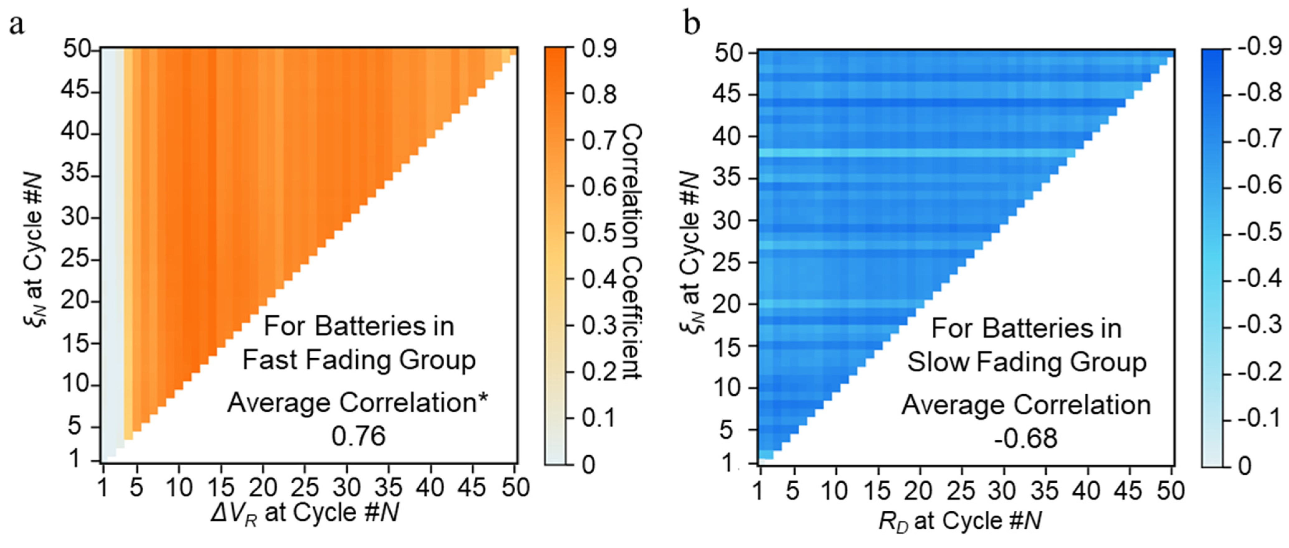
5.2. Capacity Fading Prediction

With the unsupervised Fading Mechanism Classification algorithm, the batteries are clustered into two groups using a single feature from the second cycle. For batteries in the Fast Fading Group, their capacity loss is mainly caused by the “dead” Li, which forms during charging under a high charging rate. Although ∆V_R is determined by the evolution of the surface lithium–ion concentration in both the oxide cathode and graphite anode, the contribution from the graphite anode is negligible because its surface concentration remains invariant due to the reaction between the plated Li and graphite. Therefore, a much smaller ∆V_R is observed than in batteries without Li plating. With an invariant electrochemical potential from the graphite electrode, the voltage drops after charging comes from the relaxation of the oxide. Additionally, a larger ∆V_R indicates a steeper concentration gradient in the oxide cathode after charging, corresponding to a more stringent charging condition and more severe Li plating. Therefore, it is expected that ∆V_R correlates positively with the average capacity fading rate. This conclusion, drawn from the physical analysis, is supported by the correlation analysis shown in Figure 4a. Figure 4a shows the correlation between the average capacity fading rate and ∆V_R for all batteries in the Fast Fading Group. For most of the region, the correlation is greater than 0.75, which indicates that a battery with a larger ∆V_R will have a larger ${\xi }_N$ at the Nth cycle. This positive correlation corresponds to our physics insight that a larger ∆V_R is related to more plated Li and a larger ${\xi }_N$. However, in some regions, particularly with ∆V_R obtained from the first four cycles, the correlation is relatively low due to the battery experiencing a relatively weak Li plating reaction. In the early cycles, Li plating does occur in these batteries; however, other fading mechanisms also contribute to degradation, affecting the correlation between ∆V_R and the capacity fading rate. As degradation progresses and Li plating becomes more dominant, the correlation strengthens (see Supplementary Materials Note S8). As the actual capacity decreases, the actual charging environment will deteriorate for a battery dominated by Li plating, given a fixed charging current and an increased actual C–rate. In other words, the relationship between the average capacity fading rate and ∆V_R only develops after the situation worsens sufficiently. In this case, it occurs after the first four cycles. Overall, a mean correlation of 0.76 is observed after excluding the first four cycles, indicating a strong positive correlation between ∆V_R and ${\xi }_N$. Therefore, ∆V_R is used as a key feature in constructing a regression model (Fading Prediction Module A) to accurately predict the capacity fading rate for batteries in the Fast Fading Group.

For batteries in the Slow Fading Group, given that their capacity fading is governed by SEI growth, the best feature for predicting capacity fading should contain the characteristics of the SEI growth physics. During battery cycling, the SEI grows by irreversible decomposition of the electrolyte. This process consumes the usable lithium ion in the battery and leads to capacity loss. Meanwhile, as the SEI grows thicker, its resistance to current, R_SEI, increases accordingly. Therefore, more capacity loss means a higher R_SEI. In other words, R_SEI correlates positively with the capacity fading rate. Since R_SEI cannot be measured directly during battery cycling, an equivalent resistance must be computed from the V(t) profiles to approximate R_SEI. For this purpose, we first examine the physics governing the battery voltage (Equation (9)). During discharge, the battery voltage is the difference between the equilibrium voltage V_Eq and the total overpotential, including the ohmic, the reaction overpotential, the electrolyte concentration overpotential, and the SEI overpotential. The former three can be assumed to be invariant between cycles, given that SEI growth has a negligible influence on them. In addition, V_Eq is also invariant between cycles since all the batteries are discharged from the same SOC. Therefore, the V(t) profile change during the discharge stage is only attributed to SEI growth. For this reason, the computed average resistance during the discharge process is used to approximate the R_SEI (Equation (10)). With these two equations, we can derive and conclude that there is a linear negative relationship between R_D and R_SEI (Equation (11)).

$$V_{Bat}=V_{Eq}-{\eta }_{ohim,e}-{\eta }_{rxn}-{\eta }_e-{\eta }_{SEI}$$

(9)

$$R_D\left(N\right)={\displaystyle \frac{1}{t}}{\displaystyle \underset{0}{\overset{t}{\int }}\frac{V_{Bat}\left(N\right)}{I_D}}\mathrm{dt}$$

(10)

$$R_D\left(N\right)={\displaystyle \frac{1}{t}}{\displaystyle \underset{0}{\overset{t}{\int }}\frac{C-{\eta }_{SEI}\left(N\right)}{I_D}}\mathrm{dt}=C-{\displaystyle \frac{{\eta }_{SEI}\left(N\right)}{I_D}}~-R_{SEI}\left(N\right)$$

(11)

Based on the above physical analysis, R_D is the average resistance during the discharge process. For batteries in the Slow Fading Group, the polarization effect from charging diminishes much faster compared to the Fast Fading Group. Consequently, after the resting stage, the polarization effect from charging can be disregarded. However, the polarization progressively increases during discharge. To minimize the impact of discharge–induced polarization, R_D is calculated using the data from the first three seconds. It is expected that R_D correlates linearly with ${\xi }_N$. To verify this assumption, for all batteries in the Slow Fading Group, a correlation plot between R_D and ${\xi }_N$ at different cycles is presented (Figure 4b). For most regions, the correlation between R_SEI and ${\mathsf{\xi }}_N$ is lower than −0.68, confirming the strong negative correlation between R_D and capacity fading. For this reason, R_D will be used as the feature to construct a regression model (Fading Prediction Module B) to predict ${\mathsf{\xi }}_N$ for batteries classified as the Slow Fading Group.

Next, we present the machine learning modules with ∆V_R and R_D as the features to predict the capacity fading for batteries in either the Fast Fading Group or Slow Fading Group and show their prediction results. The objective of the regression model is to forecast the average capacity fading rate at the 50th cycle (${\xi }_{50}$) of a battery charged with a specific charging protocol using data from early cycles. The model uses ∆V_R (for batteries in the Fast Fading Group) and R_D (for batteries in the Slow Fading Group). Due to the previously mentioned poor relationship between ${\xi }_{50}$ and ∆V_R for the Fast Fading Group in the first four cycles, R_D and ∆V_R are obtained from the fifth cycle.

Such an assessment of the charging protocol using data only from the early cycles can significantly improve the efficiency of the optimization of the charging protocol and shorten the cycle test time. Given the limited dataset, linear SVR is used. SVR can balance the model complexity and prediction error by incorporating an ℇ–insensitive region within the optimization problem, providing excellent generalization ability and high prediction accuracy. In comparison, a deep learning model, such as a deep neural network involving many training parameters, needs a large dataset for model training, which is not applicable in this study. In this study, a 70/30 training/test split on the dataset was used. The training data contains 19 batteries from the Fast Fading Group and 10 batteries from the Slow Fading Group. The testing data includes nine batteries and five batteries from the Fast Fading Group and Slow Fading Group, respectively. Furthermore, to avoid over–fitting on the training dataset, k–fold cross–validation was performed to choose the hyper–parameters. Various k values are evaluated, with the results showing that 5–fold cross–validation provides the best result.

To demonstrate the predictability of the physics–guided features, single––feature regression models are developed with ∆V_R and R_D from the fifth cycle, respectively. A previously reported model, the Variance model, which also utilizes one feature, is used as the benchmark to validate the proposed framework. According to Severson et al., the log variance of the discharging curve difference ∆Q_N−1(V) is selected due to its strong correlation with the predicted features [8]. The parity plots of the actual and predicted ${\xi }_{50}$ are demonstrated in Figure 5a (Fading Prediction Module A for the Fast Fading Group and Fading Prediction Module B for the Slow Fading Group), while Figure 5b presents the error distribution. In contrast, for the benchmark model, the parity plot and the prediction error are presented in Figure 5c and Figure 5d, respectively. According to parity plots, the Variance model performs relatively poorly because of the high prediction error for batteries with a low capacity fade rate. This indicates that the selected features, log ∆Q_5–1(V), cannot determine the dominant fading mechanism. This error is also shown by the distribution of the mean absolute percentage error (MAPE) in the histogram in Figure 5d. In the Variance model, for batteries classified as slow fading in the test set, the maximum absolute percentage error reaches 1201.13%, and the corresponding mean MAPE is 480.69%. The poor performance indicates that the benchmark fails to make capacity fading rate predictions for batteries classified in the Slow Fading Group. In contrast, the proposed model can avoid this problem by first discerning the dominant capacity fading mechanism. By selecting specific physics–guided features, ∆V_R and R_D, for each group, we achieve an overall test MAPE of 27.96%. In contrast, because the selected features, log ∆Q_5–1(V), cannot determine the dominant fading mechanism, the Variance model has a 192.61% test MAPE, which is significantly higher than that of the proposed framework.

In addition to the selected features, other physics–guided features have been added to improve prediction accuracy further. For LiBs, the Faraday efficiency describes the efficiency with which electrons are transferred in batteries. Therefore, it can be used to tell how many electrons are consumed by the side reactions which are directly related to capacity loss. By assuming a linear relationship between the geometric average Faraday efficiency of cycle N₁ and N₂, we can calculate the prospective cumulative Faraday efficiency of cycle N₂ to reflect capacity loss (see Supplementary Materials Note S3). Moreover, the average capacity fading rate at the fifth cycle, ${\xi }_5$, is added as the third feature to provide the model with previous fading information.

Two state–of–the–art models are introduced [8,14] to validate the proposed method. These two models target early–stage battery lifetime prediction. In contrast to the proposed model, these models do not have a dominant fading mechanism classifier. Therefore, relevant features are extracted following prediction. However, at the same time, the selected features and proposed models are different (see Supplementary Material Table S3).

(1)

Discharge model. In [8], the authors proposed three models to predict battery lifetime. The model with six features, derived from first–100–cycle data, provided the best prediction result with an elastic net regression model. We reproduce these features using the first–5–cycle degradation data.

(2)

General Regression Neural Network (GRNN). In [14], based on the importance ranking of all features, four features derived from first–100–cycle data were selected and input into a GRNN model. However, the fourth feature, the increase in internal resistance, is not included in our dataset. Therefore, three features are reproduced with our dataset and fed into a GRNN model.

Tree–based regression has also been used to forecast battery lifespan [33]. The proposed framework, which includes a clustering method to determine a primary fading mechanism followed by regression, is similar to tree–based regression. Consequently, a random forest regression (RFR) technique has been incorporated as a benchmark with ∆V_R, R_D, prospective cumulative Faraday efficiency, and ${\xi }_5$. The prospective cumulative Faraday efficiency and ${\xi }_5$ are added to the Variance model, which denotes as Variance–M. Furthermore, three naïve models are also added (Supplementary Materials Table S2). To ensure a robust model evaluation, we performed 10 random train–test splits. A comparison of the mean test errors between the proposed framework and other models is summarized in Figure 6. With the help of two extra features, prospective Faraday efficiency and ${\xi }_5$, for the proposed method, the test MAPE is reduced to 17.09% while the test RMSE is at 0.09%/cycle. In contrast, the Discharge model only achieves a test MAPE of 206.15% and a test RMSE of 0.11%/cycle. The GRNN model has a test MAPE of 73.13% and a test RMSE of 0.11%/cycle. The RFR performs relatively well, which suggests that it is important to separate the battery. Among the nine models, the proposed method has the lowest test MAPE and outperforms all other benchmarks, including three naïve models. As for the test RMSE, the Variance–M provides the lowest RMSE of 0.08%/cycle while the proposed model has a comparable value at 0.09%/cycle. The relatively low performance at the test RMSE can be attributed to the distinctive and large difference in fading behavior between the Fast Fading Group and the Slow Fading Group. The RMSE is skewed by the high average capacity fading rate in the Fast Fading Group. Therefore, the Variance–M model tends to fit the batteries with a higher average fading rate to lower the fitting error while accepting a significant percentage error in the Slowing Fading Group, resulting in a small test RMSE and large test MAPE (see Supplementary Materials Table S3).

6. Discussion

Our work aims to use the physical mechanism to guide the feature selection and use a data–driven method to describe the relationship between physics–based inputs, (1) ∆V_R and the dominant capacity fading mechanism and (2) ∆V_R and R_D, and the target output, ${\xi }_N$. In our work, inspired by the two different fading mechanisms within Li–ion batteries, a fading mechanism classification is performed to determine which fading mechanism is dominant before making a capacity fading prediction. However, it is worth noting that there are cases where the classifier fails to describe the dominant fading mechanism. As mentioned in the previous paragraph and shown by many studies, for Li plating to occur, the battery must operate at a high current ratio with respect to its present capacity and active lithium–ion concentration [32,34,35,36,37]. For a fresh battery, due to its relatively small loss of active Li–ion, the operating environment is not harsh enough to reduce and deposit sufficient Li, which leads to an incorrect classification result. However, this situation only occurs in a few batteries and can be avoided by selecting ∆V_R from later cycles. The selected feature ∆V_R provides a distinctive classification result even with data obtained from the second cycle and achieves 95.6% accuracy. This highlights the importance of physics–guided insights in model development. Due to the different characteristics of these two fading mechanisms, growth of SEI and Li plating, physics–guided data characterization is performed, and two features, ∆V_R and R_D, are extracted from the cycle data. Along with other physical features, prospective cumulative Faraday efficiency, and past average capacity fading rate, regression models for each group have a good performance given five cycles data, compared to that of the Variance–M, which uses the log variance of $\mathsf{\Delta }{Q}_{N-1}\left(V\right)$ for all batteries. The reason for the accurate results and good extrapolation of these regression models with selected features can be summarized by two factors. (1) Thanks to the dominant fading mechanism classifier, in the proposed model, each regression module is responsible for one fading mechanism with corresponding physics–guided features. In contrast, the Variance–M tried to generate a model that fit both fading mechanisms, leading to poor performance for batteries classified as the Slow Fading Group. (2) The physics–guided data characterization provides the model with good extrapolation and generalizability. Therefore, even though only five cycles are given, the regression model still outperforms all benchmarks. Moreover, the selected features can be easily obtained in the filed application, ∆V_R can be obtained from the short rest immediately after the high constant current charging, while R_D can be acquired once the battery is discharged after a rest period.

7. Conclusions

In this study, we proposed a physics–guided, data–driven model designed to predict capacity fading under fast charge conditions for Li–ion batteries. With an understanding of battery physics, the framework includes a classifier to identify the dominant battery fading mechanism and two regressors tailored to predict battery capacity fading based on the identified mechanism. Inspired by the two capacity fading mechanisms, SEI growth, and Li plating, and guided by an understanding of battery physics, we use a physics–guided feature, ∆V_R, which represents the voltage drop during the rest period after charging. This feature effectively captures the potential relaxation process and is used to identify the dominant fading mechanism. We then classify the batteries into two groups: the Fast Fading Group and the Slow Fading Group. With the ∆V_R obtained from the second cycle, we achieve an accuracy of 95.6%. Following the clustering, there is a corresponding capacity fading prediction model for each fading mechanism. With two additional physics–guided features, the proposed method achieved an overall test MAPE of 17.09% and test RMSE of 0.09%/cycle. In contrast, the state–of–art models, the Discharge model, and GRNN, have a test MAPE of 206.15% and 73.13%, respectively. The poor performance of these two models is caused by the inability to discern the dominant fading mechanism, which leads to poor performance of batteries with a slow fading rate. Moreover, because the model is based on electrochemical principles, it is expected that physics–guided features can still capture fading mechanisms such as SEI growth and Li plating. Consequently, the proposed model has the potential to be applied to other types of lithium–ion batteries with different chemistries, which remains a subject for future validation. Moreover, other fading modes, such as the loss of active materials and conductivity loss, should also be considered in future work.

References

- Xiong, W.; Mo, Y.; Yan, C. Lithium–Ion Battery Parameters and State of Charge Joint Estimation Using Bias Compensation Least Squares and the Alternate Algorithm. Math. Probl. Eng. 2020, 2020, 1DUMMMY. [Google Scholar] [CrossRef]
- Schmalstieg, J.; Käbitz, S.; Ecker, M.; Sauer, D.U. A Holistic Aging Model for Li(NiMnCo)O2 Based 18650 Lithium–Ion Batteries. J. Power Sources 2014, 257, 325–334. [Google Scholar] [CrossRef]
- Broussely, M.; Herreyre, S.; Biensan, P.; Kasztejna, P.; Nechev, K.; Staniewicz, R.J. Aging Mechanism in Li Ion Cells and Calendar Life Predictions. J. Power Sources 2001, 97–98, 13–21. [Google Scholar] [CrossRef]
- Sulzer, V.; Marquis, S.G.; Timms, R.; Robinson, M.; Chapman, S.J. Python Battery Mathematical Modelling (PyBaMM). J. Open Res. Softw. 2021, 9, 1–8. [Google Scholar] [CrossRef]
- Yan, L.; Peng, J.; Gao, D.; Wu, Y.; Liu, Y.; Li, H.; Liu, W.; Huang, Z. A Hybrid Method with Cascaded Structure for Early–Stage Remaining Useful Life Prediction of Lithium–Ion Battery. Energy 2022, 243, 123038. [Google Scholar] [CrossRef]
- Tang, X.; Liu, K.; Wang, X.; Liu, B.; Gao, F.; Widanage, W.D. Real–Time Aging Trajectory Prediction Using a Base Model–Oriented Gradient–Correction Particle Filter for Lithium–Ion Batteries. J. Power Sources 2019, 440, 227118. [Google Scholar] [CrossRef]
- Xiong, W.; Xu, G.; Li, Y.; Zhang, F.; Ye, P.; Li, B. Early Prediction of Lithium–Ion Battery Cycle Life Based on Voltage–Capacity Discharge Curves. J. Energy Storage 2023, 62, 106790. [Google Scholar] [CrossRef]
- Severson, K.A.; Attia, P.M.; Jin, N.; Perkins, N.; Jiang, B.; Yang, Z.; Chen, M.H.; Aykol, M.; Herring, P.K.; Fraggedakis, D.; et al. Data–Driven Prediction of Battery Cycle Life before Capacity Degradation. Nat. Energy 2019, 4, 383–391, ISBN 4156001903. [Google Scholar] [CrossRef]
- Attia, P.M.; Severson, K.A.; Witmer, J.D. Statistical Learning for Accurate and Interpretable Battery Lifetime Prediction. J. Electrochem. Soc. 2021, 168, 090547. [Google Scholar] [CrossRef]
- Li, X.; Wang, Z.; Yan, J. Prognostic Health Condition for Lithium Battery Using the Partial Incremental Capacity and Gaussian Process Regression. J. Power Sources 2019, 421, 56–67. [Google Scholar] [CrossRef]
- Richardson, R.R.; Osborne, M.A.; Howey, D.A. Gaussian Process Regression for Forecasting Battery State of Health. J. Power Sources 2017, 357, 209–219. [Google Scholar] [CrossRef]
- Gao, D.; Huang, M. Prediction of Remaining Useful Life of Lithium–Ion Battery Based on Multi–Kernel Support Vector Machine with Particle Swarm Optimization. J. Power Electron. 2017, 17, 1288–1297. [Google Scholar] [CrossRef]
- Fei, Z.; Zhang, Z.; Yang, F.; Tsui, K.L.; Li, L. Early–Stage Lifetime Prediction for Lithium–Ion Batteries: A Deep Learning Framework Jointly Considering Machine–Learned and Handcrafted Data Features. J. Energy Storage 2022, 52, 104936. [Google Scholar] [CrossRef]
- Zhang, Y.; Peng, Z.; Guan, Y.; Wu, L. Prognostics of Battery Cycle Life in the Early–Cycle Stage Based on Hybrid Model. Energy 2021, 221, 119901. [Google Scholar] [CrossRef]
- Xu, F.; Yang, F.; Fei, Z.; Huang, Z.; Tsui, K.L. Life Prediction of Lithium–Ion Batteries Based on Stacked Denoising Autoencoders. Reliab. Eng. Syst. Saf. 2021, 208, 107396. [Google Scholar] [CrossRef]
- Yao, J.; Powell, K.; Gao, T. A two-stage deep learning framework for early-stage lifetime prediction for lithium-ion batteries with consideration of features from multiple cycles. Front. Energy Res. 2020, 10, 1059126. [Google Scholar]
- Hsu, C.W.; Xiong, R.; Chen, N.Y.; Li, J.; Tsou, N.T. Deep Neural Network Battery Life and Voltage Prediction by Using Data of One Cycle Only. Appl. Energy 2022, 306, 118134. [Google Scholar] [CrossRef]
- Aykol, M.; Gopal, C.B.; Anapolsky, A.; Herring, P.K.; van Vlijmen, B.; Berliner, M.D.; Bazant, M.Z.; Braatz, R.D.; Chueh, W.C.; Storey, B.D. Perspective—Combining Physics and Machine Learning to Predict Battery Lifetime. J. Electrochem. Soc. 2021, 168, 030525. [Google Scholar] [CrossRef]
- Thelen, A.; Lui, Y.H.; Shen, S.; Laflamme, S.; Hu, S.; Ye, H.; Hu, C. Integrating Physics–Based Modeling and Machine Learning for Degradation Diagnostics of Lithium–Ion Batteries. Energy Storage Mater. 2022, 50, 668–695. [Google Scholar] [CrossRef]
- Najera–Flores, D.A.; Hu, Z.; Chadha, M.; Todd, M.D. A Physics–Constrained Bayesian Neural Network for Battery Remaining Useful Life Prediction. Appl. Math. Model. 2023, 122, 42–59. [Google Scholar] [CrossRef]
- Shi, J.; Rivera, A.; Wu, D. Battery Health Management Using Physics–Informed Machine Learning: Online Degradation Modeling and Remaining Useful Life Prediction. Mech. Syst. Signal Process. 2022, 179, 109347. [Google Scholar] [CrossRef]
- Deng, Z.; Lin, X.; Cai, J.; Hu, X. Battery Health Estimation with Degradation Pattern Recognition and Transfer Learning. J. Power Sources 2022, 525, 231027. [Google Scholar] [CrossRef]
- Jiang, B.; Gent, W.E.; Mohr, F.; Ermon, S.; Chueh, W.C.; Richard, D.; Jiang, B.; Gent, W.E.; Mohr, F.; Das, S.; et al. Bayesian Learning for Rapid Prediction of Lithium–Ion Battery–Cycling Protocols of Lithium–Ion Battery–Cycling Protocols. Joule 2021, 5, 3187–3203. [Google Scholar] [CrossRef]
- Chen, B.R.; Kunz, M.R.; Tanim, T.R.; Dufek, E.J. A Machine Learning Framework for Early Detection of Lithium Plating Combining Multiple Physics–Based Electrochemical Signatures. Cell Reports Phys. Sci. 2021, 2, 100352. [Google Scholar] [CrossRef]
- Chen, B.R.; Walker, C.M.; Kim, S.; Kunz, M.R.; Tanim, T.R.; Dufek, E.J. Battery Aging Mode Identification across NMC Compositions and Designs Using Machine Learning. Joule 2022, 6, 2776–2793. [Google Scholar] [CrossRef]
- Ansean, D.; Garcia, V.M.; Gonzalez, M.; Blanco–Viejo, C.; Viera, J.C.; Pulido, Y.F.; Sanchez, L. Lithium–Ion Battery Degradation Indicators Via Incremental Capacity Analysis. IEEE Trans. Ind. Appl. 2019, 55, 2992–3002. [Google Scholar] [CrossRef]
- Ahmed, M.; Seraj, R.; Islam, S.M.S. The K–Means Algorithm: A Comprehensive Survey and Performance Evaluation. Electron. 2020, 9, 1295. [Google Scholar] [CrossRef]
- Cortes, C.; Vapnik, V. Support–Vector Networks. Mach. Learn. 1995, 20, 273–297. [Google Scholar] [CrossRef]
- Drucker, H.; Surges, C.J.C.; Kaufman, L.; Smola, A.; Vapnik, V. Support Vector Regression Machines. Adv. Neural Inf. Process. Syst. 1997, 1, 155–161. [Google Scholar]
- Smola, A.J.; Schölkopf, B. A Tutorial on Support Vector Regression. Stat. Comput. 2004, 14, 199–222. [Google Scholar] [CrossRef]
- Pinson, M.B.; Bazant, M.Z. Theory of SEI Formation in Rechargeable Batteries: Capacity Fade, Accelerated Aging and Lifetime Prediction. J. Electrochem. Soc. 2013, 160, A243–A250. [Google Scholar] [CrossRef]
- Gao, T.; Han, Y.; Fraggedakis, D.; Das, S.; Zhou, T.; Yeh, C.N.; Xu, S.; Chueh, W.C.; Li, J.; Bazant, M.Z. Interplay of Lithium Intercalation and Plating on a Single Graphite Particle. Joule 2021, 5, 393–414. [Google Scholar] [CrossRef]
- Chowdhury, S.; Lin, Y.; Liaw, B.; Kerby, L. Evaluation of Tree Based Regression over Multiple Linear Regression for Non–Normally Distributed Data in Battery Performance. In Proceedings of the 2022 International Conference on Intelligent Data Science Technologies and Applications (IDSTA), San Antonio, TX, USA, 5–7 September 2022; pp. 17–25. [Google Scholar] [CrossRef]
- Tanim, T.R.; Paul, P.P.; Thampy, V.; Cao, C.; Steinrück, H.G.; Nelson Weker, J.; Toney, M.F.; Dufek, E.J.; Evans, M.C.; Jansen, A.N.; et al. Heterogeneous Behavior of Lithium Plating during Extreme Fast Charging. Cell Rep. Phys. Sci. 2020, 1, 100114. [Google Scholar] [CrossRef]
- Tanim, T.R.; Dufek, E.J.; Evans, M.; Dickerson, C.; Jansen, A.N.; Polzin, B.J.; Dunlop, A.R.; Trask, S.E.; Jackman, R.; Bloom, I.; et al. Extreme Fast Charge Challenges for Lithium–Ion Battery: Variability and Positive Electrode Issues. J. Electrochem. Soc. 2019, 166, A1926–A1938. [Google Scholar] [CrossRef]
- Gallagher, K.G.; Trask, S.E.; Bauer, C.; Woehrle, T.; Lux, S.F.; Tschech, M.; Lamp, P.; Polzin, B.J.; Ha, S.; Long, B.; et al. Optimizing Areal Capacities through Understanding the Limitations of Lithium–Ion Electrodes. J. Electrochem. Soc. 2016, 163, A138–A149. [Google Scholar] [CrossRef]
- Tomaszewska, A.; Chu, Z.; Feng, X.; O’Kane, S.; Liu, X.; Chen, J.; Ji, C.; Endler, E.; Li, R.; Liu, L.; et al. Lithium–Ion Battery Fast Charging: A Review. eTransportation 2019, 1, 100011. [Google Scholar] [CrossRef]
Disclaimer/Publisher’s Note: The statements, opinions and data contained in all publications are solely those of the individual author(s) and contributor(s) and not of MDPI and/or the editor(s). MDPI and/or the editor(s) disclaim responsibility for any injury to people or property resulting from any ideas, methods, instructions or products referred to in the content. |
© 2024 by the authors. Licensee MDPI, Basel, Switzerland. This article is an open access article distributed under the terms and conditions of the Creative Commons Attribution (CC BY) license (https://creativecommons.org/licenses/by/4.0/).
Share and Cite
Yao, J.; Gao, Q.; Gao, T.; Jiang, B.; Powell, K.M. A Physics–Guided Machine Learning Approach for Capacity Fading Mechanism Detection and Fading Rate Prediction Using Early Cycle Data. Batteries 2024, 10, 283. https://doi.org/10.3390/batteries10080283
Yao J, Gao Q, Gao T, Jiang B, Powell KM. A Physics–Guided Machine Learning Approach for Capacity Fading Mechanism Detection and Fading Rate Prediction Using Early Cycle Data. Batteries. 2024; 10(8):283. https://doi.org/10.3390/batteries10080283
Chicago/Turabian StyleYao, Jiwei, Qiang Gao, Tao Gao, Benben Jiang, and Kody M. Powell. 2024. "A Physics–Guided Machine Learning Approach for Capacity Fading Mechanism Detection and Fading Rate Prediction Using Early Cycle Data" Batteries 10, no. 8: 283. https://doi.org/10.3390/batteries10080283
APA StyleYao, J., Gao, Q., Gao, T., Jiang, B., & Powell, K. M. (2024). A Physics–Guided Machine Learning Approach for Capacity Fading Mechanism Detection and Fading Rate Prediction Using Early Cycle Data. Batteries, 10(8), 283. https://doi.org/10.3390/batteries10080283