

Thermal Modelling and Temperature Estimation of a Cylindrical Lithium Iron Phosphate Cell Subjected to an Automotive Duty Cycle


Abstract
:1. Introduction
- A couple of new LFP cell electrothermal models are developed and simulated using ANSYS.
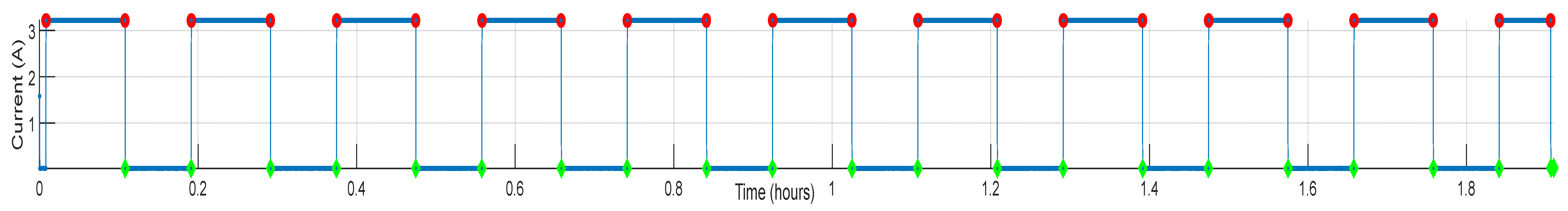
- A real automotive duty cycle is used for the validation of the proposed cell thermal model under a dynamic load profile.
- The solve design optimisation technique for ECM parameter identification is validated using experimental data, and its usability in cell temperature estimation is tested.
2. Cell Specifications and Experimental Tests
2.1. Lithium Iron Phosphate (LFP) Cell Specifications
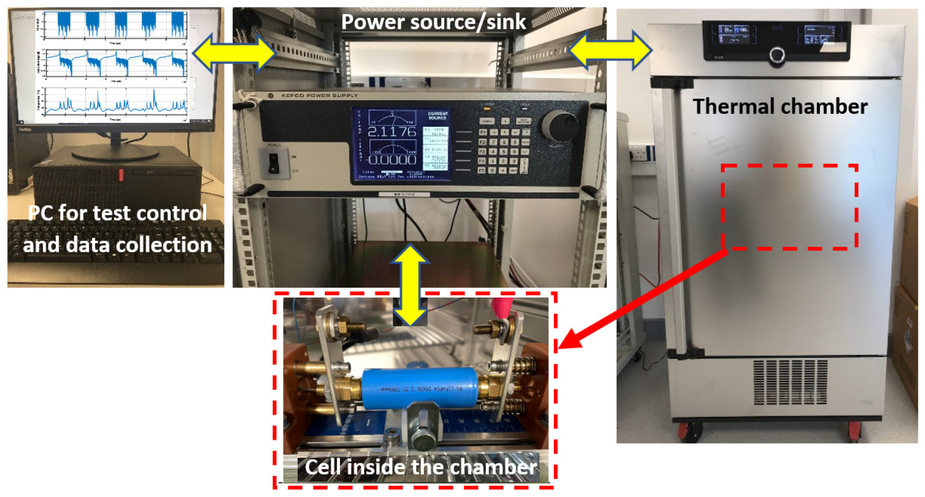
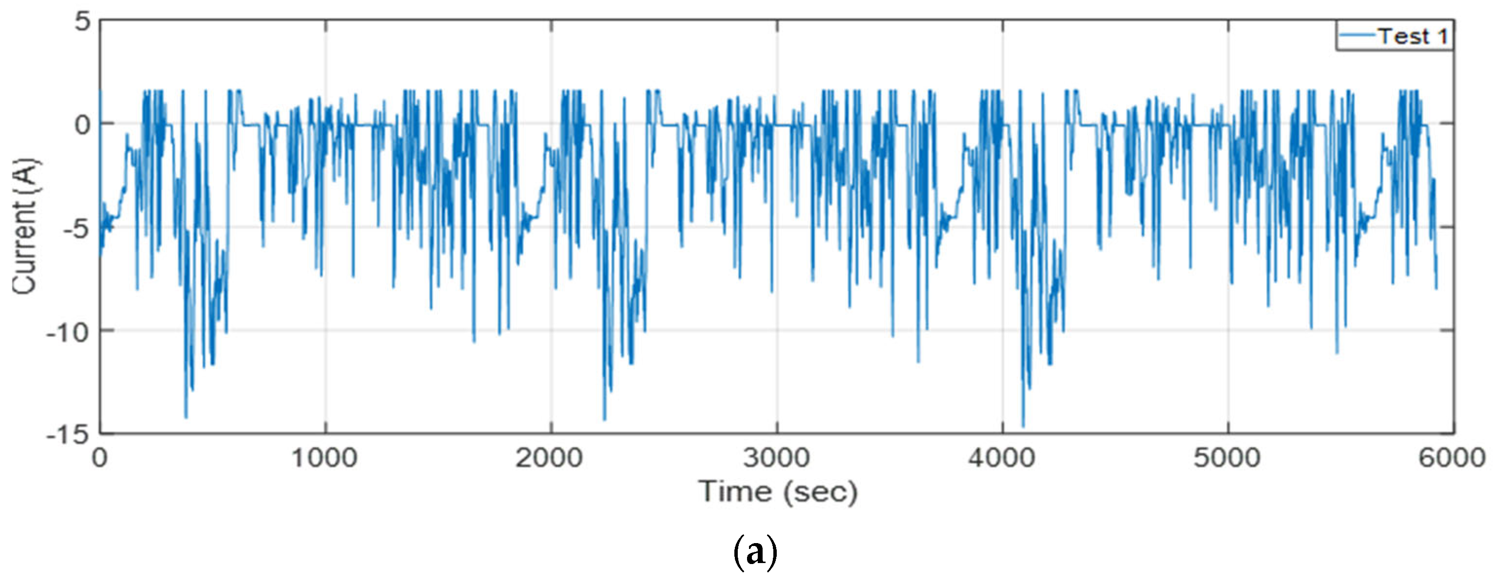
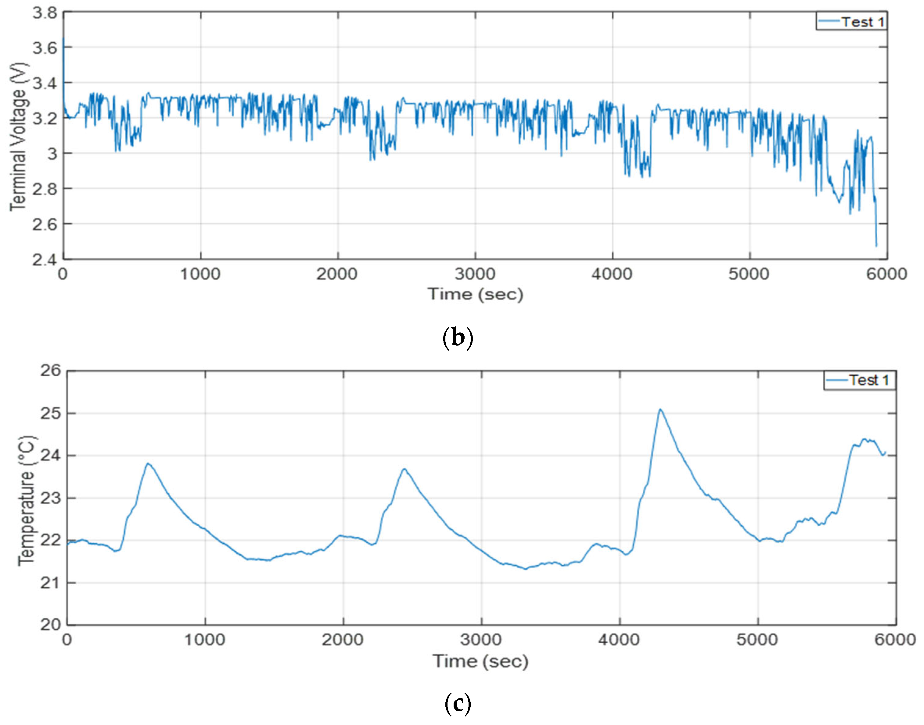
2.2. Cell Testing
3. Modelling of the LFP Cell
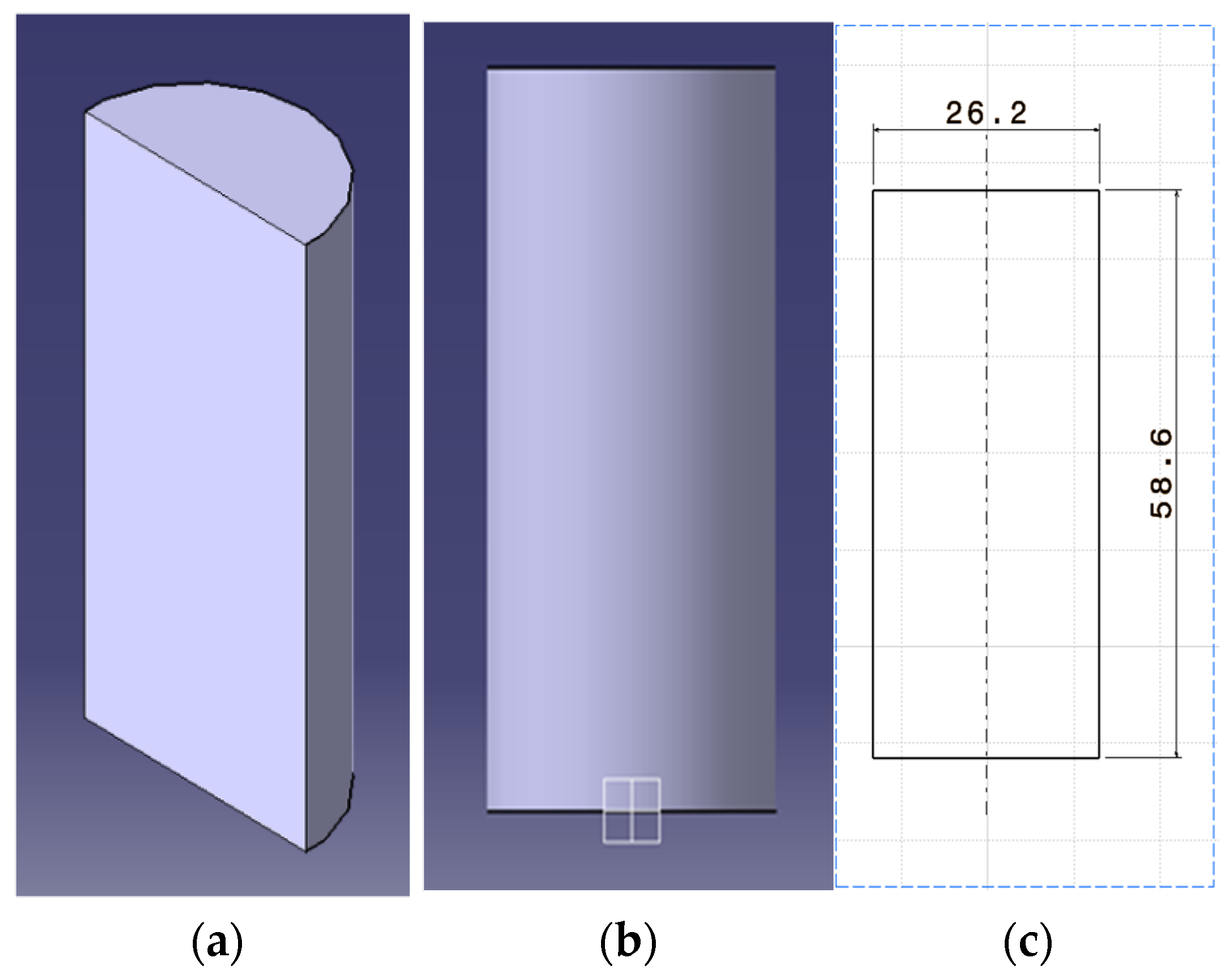
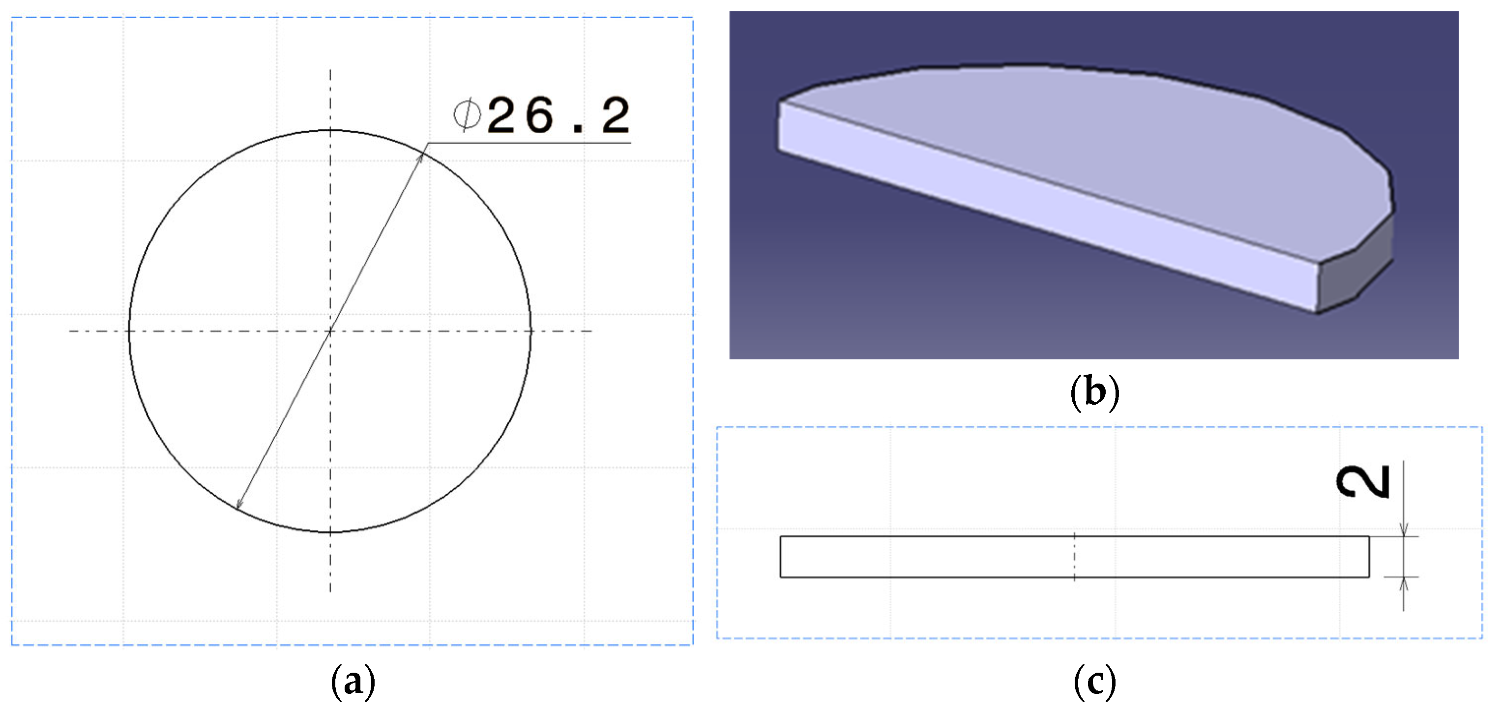
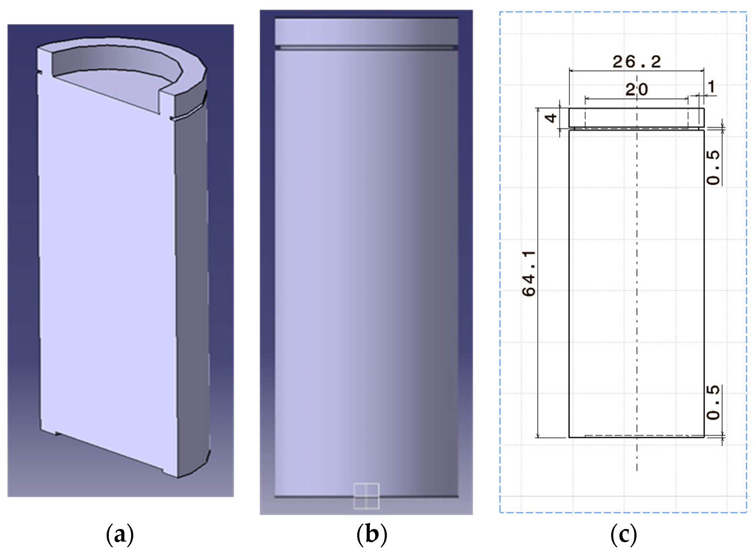
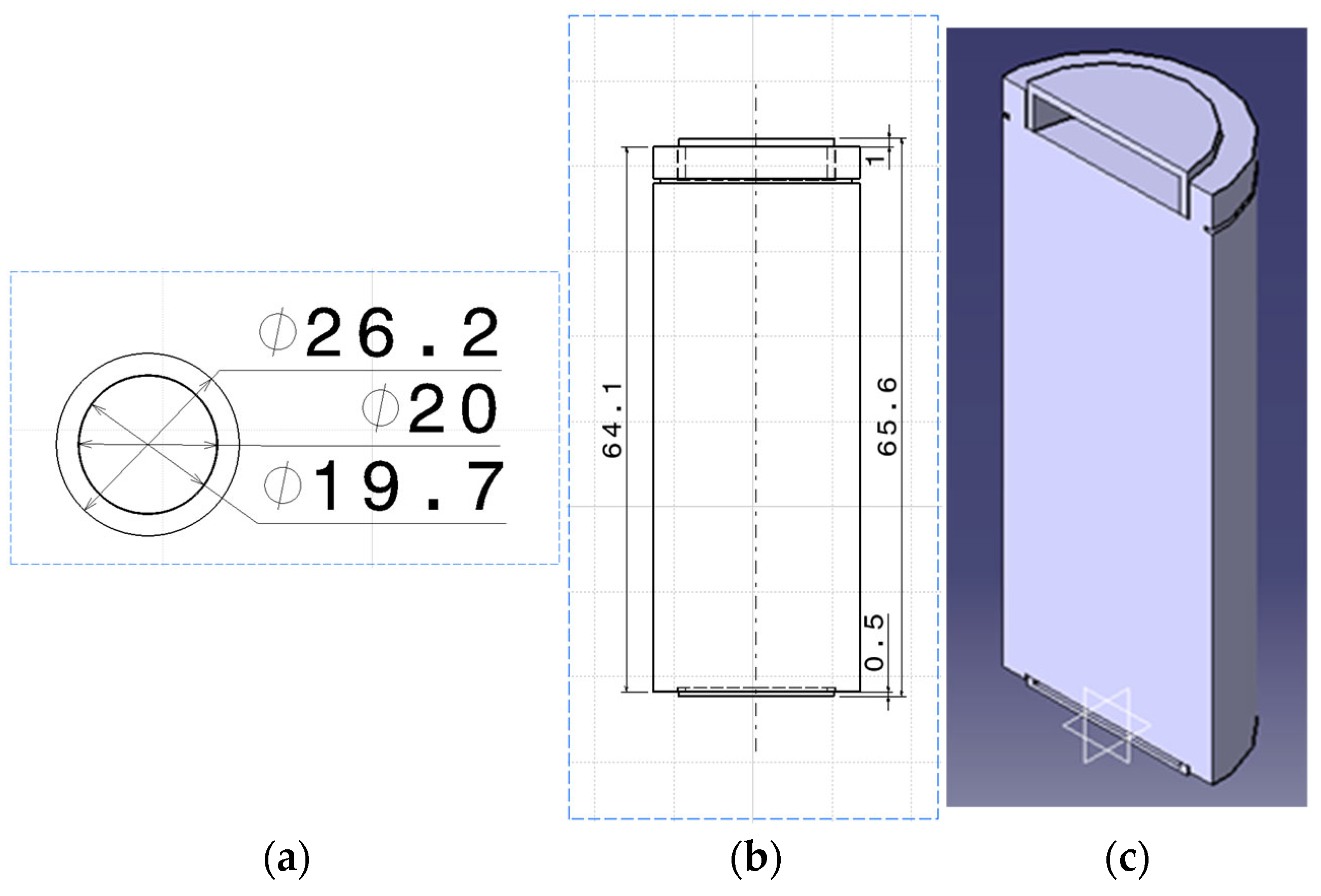
3.1. LFP Cell 3D Modelling—Iteration 1
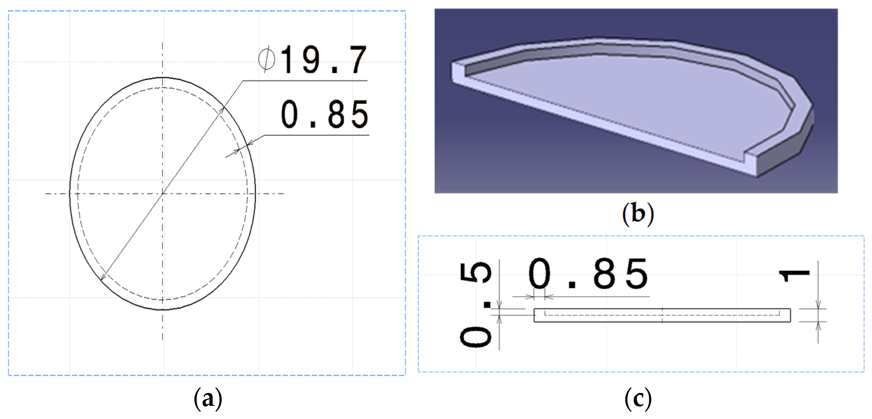
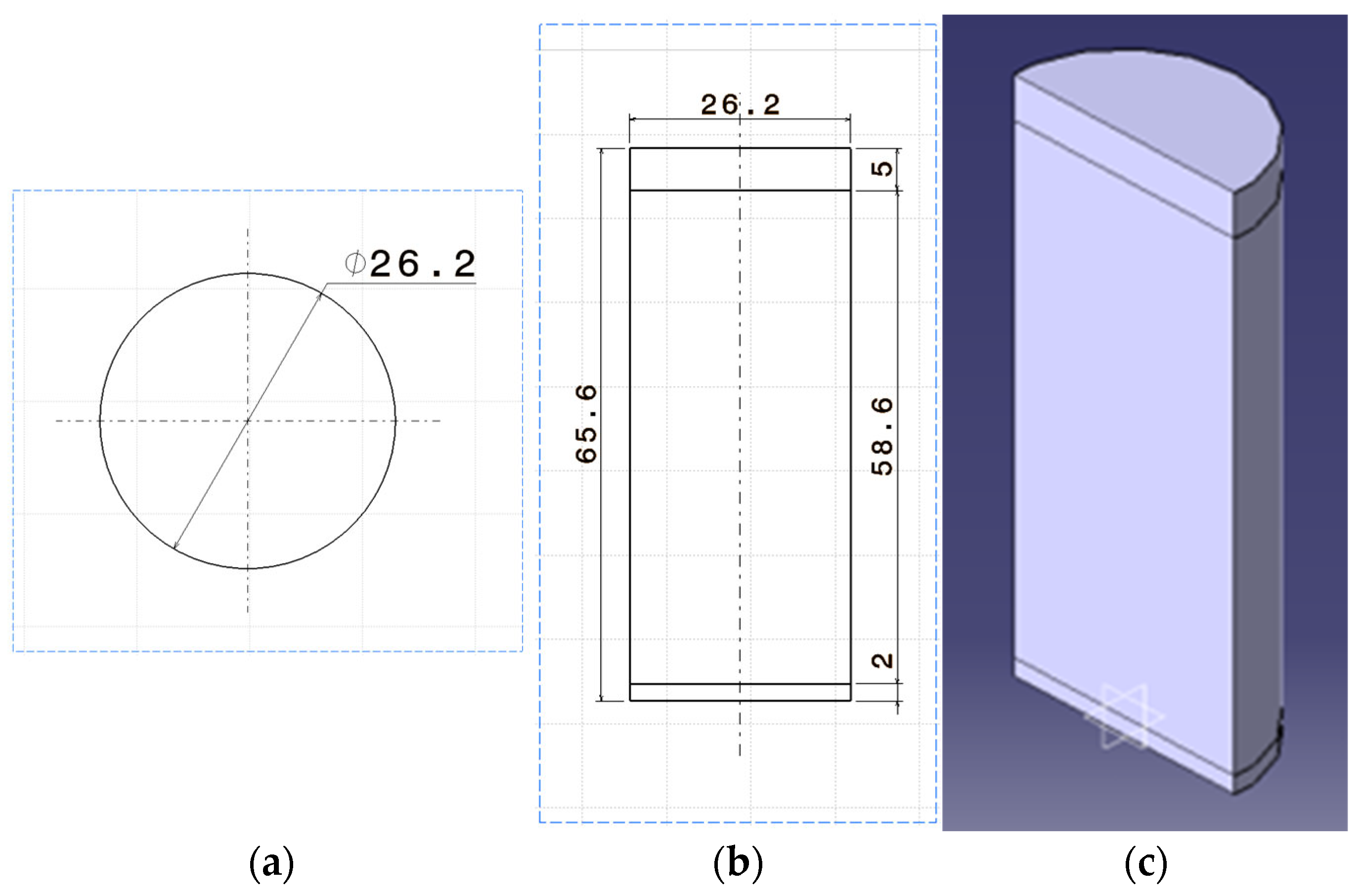
3.2. LFP Cell 3D Modelling—Iteration 2
3.3. Cell Assembly
4. Finite Element Analysis (FEA) of the LFP Cell Model
4.1. ANSYS Fluent
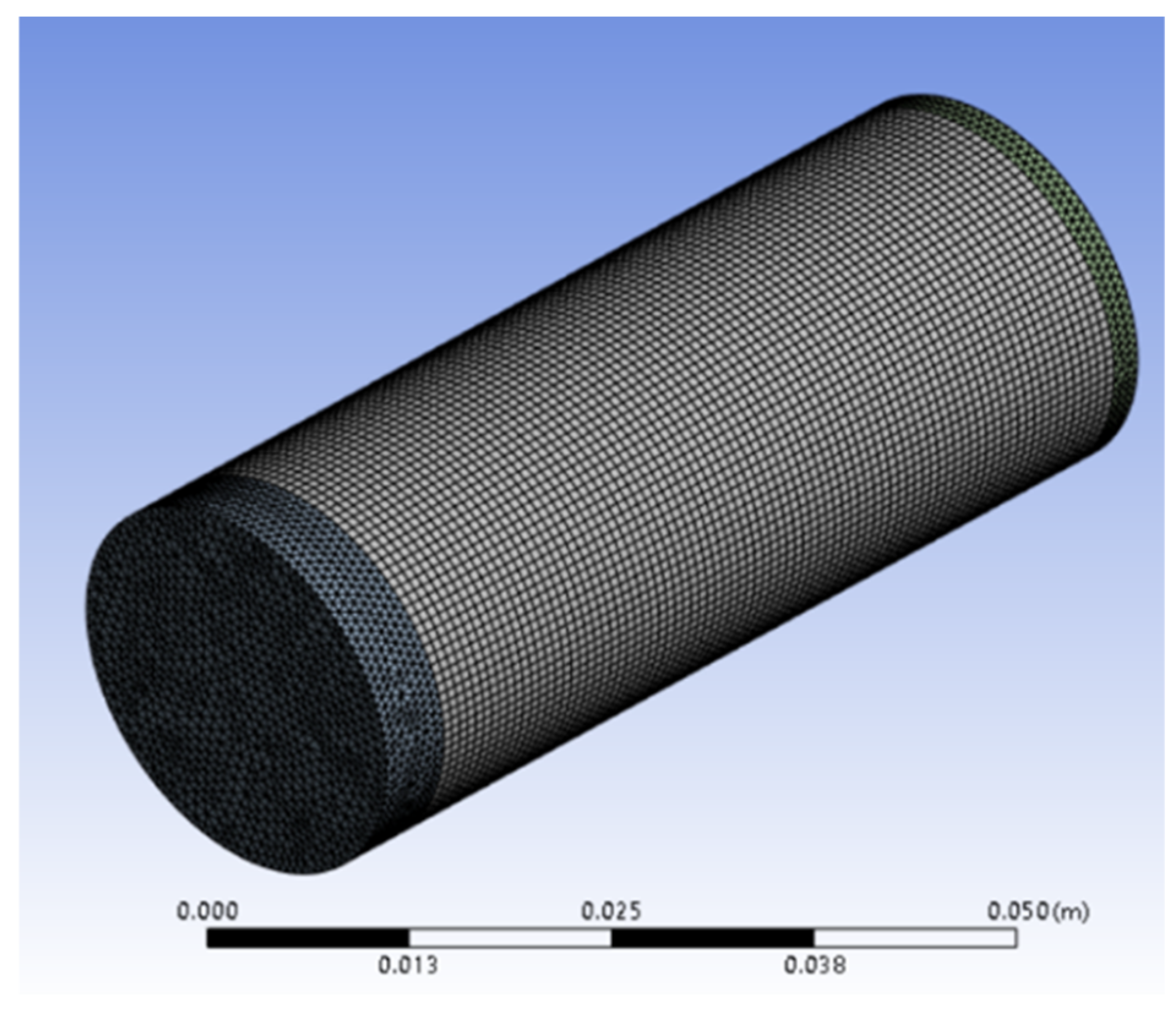
4.2. Meshing
4.2.1. LFP Cell Meshing—Iteration 1
4.2.2. LFP Cell Model Meshing—Iteration 2
4.3. Background of the Solution Method
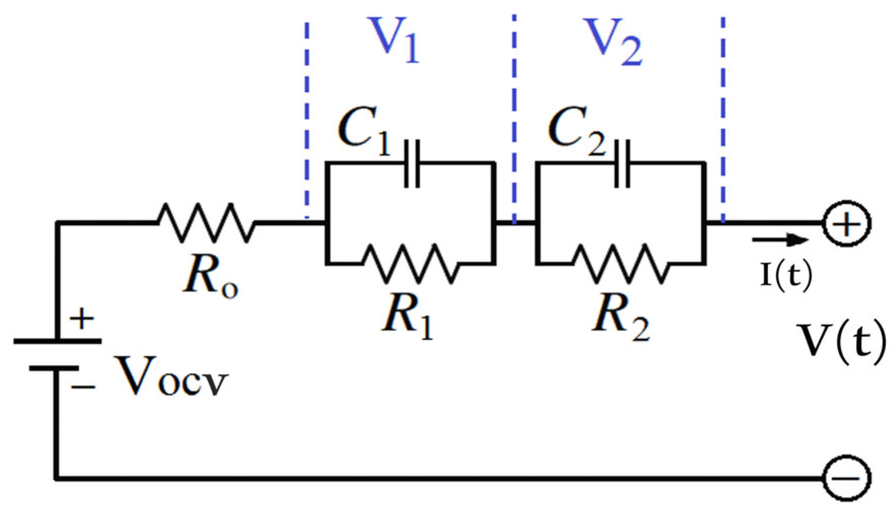
4.4. Electrical Parameters
4.5. System Identification
4.6. Material Properties
4.7. Boundary Conditions
5. Results and Discussion
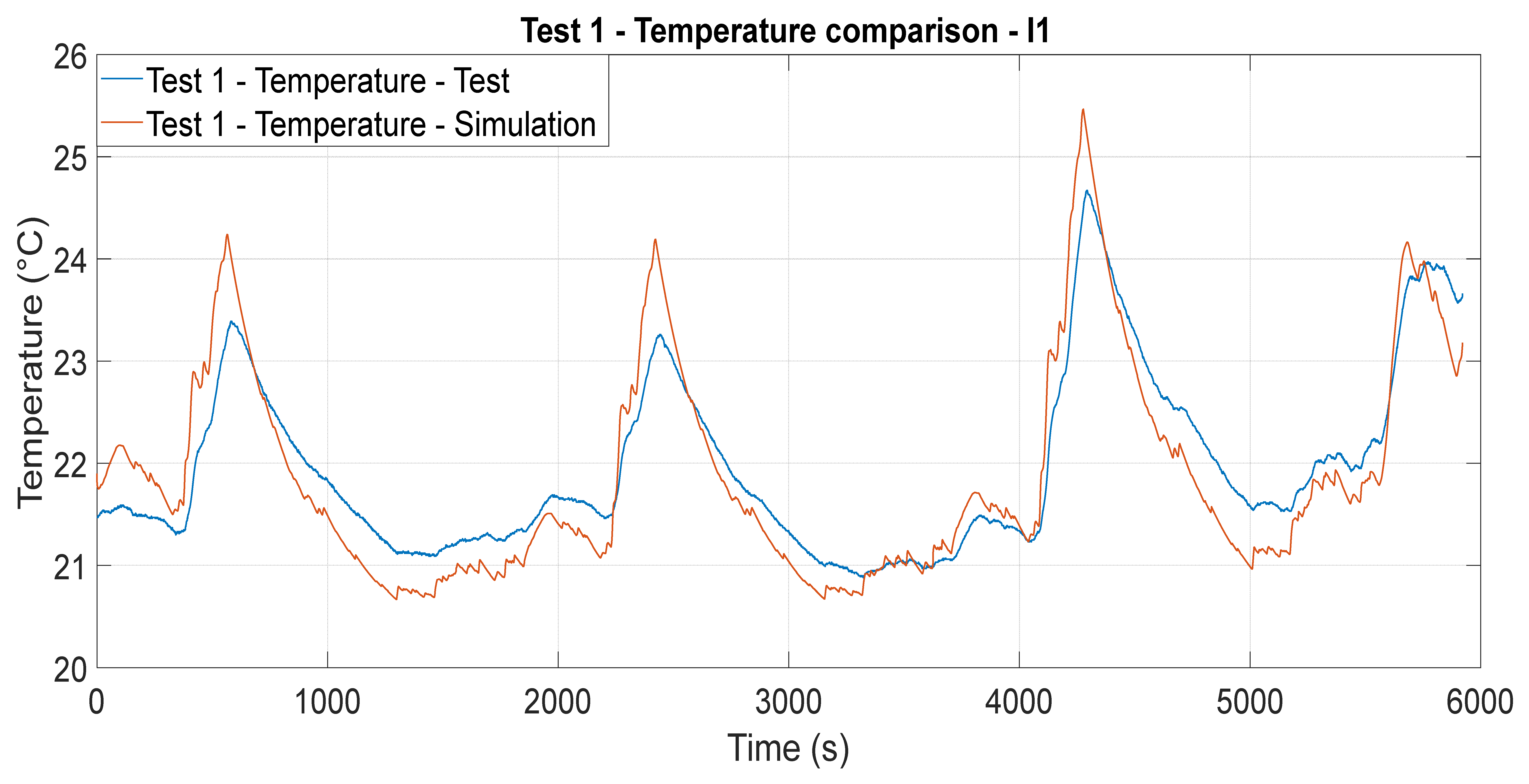
5.1. Cell Temperature Estimation—Iteration 1
5.2. Cell Temperature Estimation—Iteration 2
6. Conclusions
Author Contributions
Funding
Data Availability Statement
Conflicts of Interest
Nomenclature
| Symbols | Description |
| A | Ampere |
| Ah | Ampere-hour |
| °C | Degree Celsius |
| C1 | Polarisation capacitance (F) |
| C2 | Diffusion capacitance (F) |
| h | Heat transfer coefficient (W × m−2 × K−1) |
| I | Current (A) |
| jEch | Volumetric current transfer rate due to electrochemical reactions (A × m−3) |
| jshort | Current transfer rate due to battery internal short-circuit (A × m−3) |
| Electrochemical reaction heat(W × m−3) | |
| Heat generation rate due to battery internal short-circuit (W × m−3) | |
| Heat generation due to thermal runaway reactions under thermal abuse conditions (W × m−3) | |
| Battery total electric capacity (Ah) | |
| Reference capacity (Ah)—capacity of the battery used in tests | |
| R1 | Polarisation resistance (Ω) |
| R2 | Diffusion resistance (Ω) |
| Rs | Ohmic resistance (Ω) |
| V | Volt |
| V1 | Voltage across first resistor–capacitor network (V) |
| V2 | Voltage across second resistor–capacitor network (V) |
| VOCV | Open circuit voltage (V) |
| Vol | Active zone’s volume (m3) |
| Specific heat coefficient (J × kg−1 × K−1) | |
| Temperature (K) | |
| Thermal conductivity (W × m−1 × K−1) | |
| Equilibrium voltage (V) | |
| Greek letters | |
| σ | Effective electrical conductivity of the electrodes (S × m−1) |
| φ | Phase potential of the electrodes (V × m−1) |
| Density (kg × m−3) | |
| Acronyms | |
| 2D | Two-Dimensional |
| 3D | Three-Dimensional |
| ANSYS | Analysis System |
| BMS | Battery Management System |
| CAD | Computer-Aided Design |
| CATIA | Computer-Aided Three-Dimension Interactive Application |
| CHT | Conjugate Heat Transport |
| C-rate | Current Charge/Discharge Rate |
| ECM | Equivalent Circuit Model |
| EV | Electric Vehicle |
| FEA | Finite Element Analysis |
| FMU | Functional Mock-up Unit |
| HPPC | Hybrid Power Pulse Characterisation |
| ICE | Internal Combustion Engine |
| LFP | Lithium Iron Phosphate |
| MATLAB | MATrix LABoratory |
| MSMD | Multi-Scale Multi-Domain |
| NEDC | New European Driving Cycle |
| NTGK | Newman, Tiedeman, Gu, and Kim |
| OCV | Open Circuit Voltage |
| P2D | Pseudo-Two-Dimensional |
| PC | Personal Computer |
| PTC | Positive Thermal Coefficient |
| RC | Resistor–Capacitor |
| SDO | Solve Design Optimisation |
| SoC | State of Charge |
| UDS | User-Defined Scalar |
| WLTP | Worldwide Harmonised Light Vehicles Test Procedure |
References
- Deng, D. Li-ion batteries: Basics, progress, and challenges. Energy Sci. Eng. 2015, 3, 385–418. [Google Scholar] [CrossRef]
- Koech, A.K.; Mwandila, G.; Mulolani, F.; Mwaanga, P. Lithium-ion battery fundamentals and exploration of cathode materials: A review. S. Afr. J. Chem. Eng. 2024, 50, 321–339. [Google Scholar] [CrossRef]
- BU-205: Types of Lithium-Ion-Battery University. Available online: https://batteryuniversity.com/article/bu-205-types-of-lithium-ion (accessed on 28 November 2023).
- Khasawneh, H.; Neal, J.; Canova, M.; Guezennec, Y.; Wayne, R.; Taylor, J.; Smalc, M.; Norley, J. Analysis of Heat-Spreading Thermal Management Solutions for Lithium-Ion Batteries. In Proceedings of the ASME 2011 International Mechanical Engineering Congress and Exposition, IMECE 2011, Denver, CO, USA, 11–17 November 2011; pp. 421–428. [Google Scholar] [CrossRef]
- Bandhauer, T.M.; Garimella, S.; Fuller, T.F. A Critical Review of Thermal Issues in Lithium-Ion Batteries. J. Electrochem. Soc. 2011, 158, R1. [Google Scholar] [CrossRef]
- Saw, L.H.; Ye, Y.; Tay, A.A.O. Electrochemical-thermal analysis of 18650 Lithium Iron Phosphate cell. Energy Convers. Manag. 2013, 75, 162–174. [Google Scholar] [CrossRef]
- Ma, S.; Jiang, M.; Tao, P.; Song, C.; Wu, J.; Wang, J.; Deng, T.; Shang, W. Temperature effect and thermal impact in lithium-ion batteries: A review. Prog. Nat. Sci. Mater. Int. 2018, 28, 653–666. [Google Scholar] [CrossRef]
- Broatch, A.; Olmeda, P.; Margot, X.; Agizza, L. A generalized methodology for lithium-ion cells characterization and lumped electro-thermal modelling. Appl. Therm. Eng. 2022, 217, 119174. [Google Scholar] [CrossRef]
- Srinivasan, V.; Newman, J. Discharge Model for the Lithium Iron-Phosphate Electrode. J. Electrochem. Soc. 2004, 151, A1517. [Google Scholar] [CrossRef]
- Saw, L.H.; Ye, Y.; Tay, A.A.O. Integration issues of lithium-ion battery into electric vehicles battery pack. J. Clean. Prod. 2016, 113, 1032–1045. [Google Scholar] [CrossRef]
- Yang, Z.; Patil, D.; Fahimi, B. Electrothermal modeling of lithium-ion batteries for electric vehicles. IEEE Trans. Veh. Technol. 2019, 68, 170–179. [Google Scholar] [CrossRef]
- Liu, K.; Gao, Y.; Zhu, C.; Li, K.; Fei, M.; Peng, C.; Zhang, X.; Han, Q.-L. Electrochemical modeling and parameterization towards control-oriented management of lithium-ion batteries. Control Eng. Pract. 2022, 124, 105176. [Google Scholar] [CrossRef]
- Hu, Y.; Yurkovich, S.; Guezennec, Y.; Yurkovich, B.J. Electro-thermal battery model identification for automotive applications. J. Power Sources 2011, 196, 449–457. [Google Scholar] [CrossRef]
- Coleman, M.; Lee, C.K.; Zhu, C.; Hurley, W.G. State-of-charge determination from EMF voltage estimation: Using impedance, terminal voltage, and current for lead-acid and lithium-ion batteries. IEEE Trans. Ind. Electron. 2007, 54, 2550–2557. [Google Scholar] [CrossRef]
- Liu, Y.; Zhang, R.; Wang, J.; Wang, Y. Current and future lithium-ion battery manufacturing. iScience 2021, 24, 102332. [Google Scholar] [CrossRef] [PubMed]
- RS Pro Rechargeable Lithium Ion Iron Phosphate Battery (LiFePO4). Available online: https://uk.rs-online.com/web/p/speciality-size-rechargeable-batteries/1834305 (accessed on 18 December 2024).
- Worldwide Harmonised Light Vehicle Test Procedure|VCA. Available online: https://www.vehicle-certification-agency.gov.uk/fuel-consumption-co2/the-worldwide-harmonised-light-vehicle-test-procedure/ (accessed on 18 December 2024).
- Fotouhi, A.; Propp, K.; Auger, D.J. Electric vehicle battery model identification and state of charge estimation in real world driving cycles. In Proceedings of the 2015 7th Computer Science and Electronic Engineering Conference, CEEC 2015–Conference Proceedings, Colchester, UK, 24–25 September 2015; pp. 243–248. [Google Scholar] [CrossRef]
- Miri, I.; Fotouhi, A.; Ewin, N. Electric vehicle energy consumption modelling and estimation—A case study. Int. J. Energy Res. 2021, 45, 501–520. [Google Scholar] [CrossRef]
- Ansys Fluent User’s Guide. 2023. Available online: http://www.ansys.com (accessed on 9 March 2025).
- Jeon, D.H.; Baek, S.M. Thermal modeling of cylindrical lithium ion battery during discharge cycle. Energy Convers. Manag. 2011, 52, 2973–2981. [Google Scholar] [CrossRef]
- Kim, G.-H.; Smith, K.; Lee, K.-J.; Santhanagopalan, S.; Pesaran, A. Multi-Domain Modeling of Lithium-Ion Batteries Encompassing Multi-Physics in Varied Length Scales. J. Electrochem. Soc. 2011, 158, A955. [Google Scholar] [CrossRef]
- Chen, M.; Rincón-Mora, G.A. Accurate electrical battery model capable of predicting runtime and I-V performance. IEEE Trans. Energy Convers. 2006, 21, 504–511. [Google Scholar] [CrossRef]
- Teschner, T.-R. Lecture Notes—Grid Generation/CAD—Computational Fluid Dynamics—November 2022. 2022. Available online: www.cranfield.ac.uk (accessed on 9 March 2025).
- Arunachala, R.; Löffler, K.; Teutsch, T.; Thanagasundram, S.; Makinejad, K.; Jossen, A. A Cell Level Model for Battery Simulation. Available online: https://www.researchgate.net/publication/235602059 (accessed on 9 March 2025).
- Hua, X.; Zhang, C.; Offer, G. Finding a better fit for lithium ion batteries: A simple, novel, load dependent, modified equivalent circuit model and parameterization method. J. Power Sources 2021, 484, 229117. [Google Scholar] [CrossRef]
- Lin, X.; Perez, H.E.; Mohan, S.; Siegel, J.B.; Stefanopoulou, A.G.; Ding, Y.; Castanier, M.P. A lumped-parameter electro-thermal model for cylindrical batteries. J. Power Sources 2014, 257, 1–11. [Google Scholar] [CrossRef]
- Estimate Equivalent Circuit Lithium-Ion Battery Data-MATLAB & Simulink-MathWorks United Kingdom. Available online: https://uk.mathworks.com/help/autoblks/ug/estimate-equivalent-circuit-lithium-ion-battery-data.html (accessed on 16 October 2024).
- Lithium Battery Cell-Two RC-Branch Equivalent Circuit-MATLAB & Simulink-MathWorks United Kingdom. Available online: https://uk.mathworks.com/help/simscape/ug/lithium-battery-cell-two-rc-branch-equivalent-circuit.html (accessed on 16 October 2024).
- Kim, Y.; Siegel, J.B.; Stefanopoulou, A.G. A computationally efficient thermal model of cylindrical battery cells for the estimation of radially distributed temperatures. In Proceedings of the 2013 American Control Conference, Washington, DC, USA, 17–19 June 2013; pp. 698–703. [Google Scholar] [CrossRef]
- Ellingsen, L.A.W.; Majeau-Bettez, G.; Singh, B.; Srivastava, A.K.; Valøen, L.O.; Strømman, A.H. Life Cycle Assessment of a Lithium-Ion Battery Vehicle Pack. J. Ind. Ecol. 2014, 18, 113–124. [Google Scholar] [CrossRef]


| Specification | Value |
|---|---|
| Voltage (nominal) | 3.2 V |
| Capacity | 3300 mAh |
| Maximum cut-off voltage | 3.65 ± 0.05 V |
| Minimum cut-off voltage | 2.5 V |
| Maximum continuous discharge current | 9.6 A |
| Pulse discharge current | 15 A, 10 s |
| Operating temperature | Charging: 0–55 °C Discharging: 20–60 °C |
| Weight of the cell | 86 g |
| Mesh Metric | Optimal Value | Acceptable Value | Poor Elements |
|---|---|---|---|
| Orthogonality | 1 | 1—0.15 | <0.15 |
| Skewness | 0 | 0—0.85 | >0.85 |
| Aspect Ratio | 1 | 1—1000 | >1000 |
| Parameter | Representation | Value |
|---|---|---|
| Density | 2047 kg × m−3 | |
| Specific heat coefficient | 1109.2 J × kg−1 × K−1 | |
| Thermal conductivity | 0.610 W × m−1 × K−1 | |
| Heat transfer coefficient | h | 58.6 W × m−2 × K−1 |
| Parameter | Symbol | Value |
|---|---|---|
| Density | 2719 kg × m−3 | |
| Specific heat coefficient | 871 J × kg−1 × K−1 | |
| Thermal conductivity | 202.4 W × m−1 × K−1 |
| Parameter | Symbol | Value |
|---|---|---|
| Density | 8978 kg × m−3 | |
| Specific heat coefficient | 381 J × kg−1 × K−1 | |
| Thermal conductivity | 387.6 W × m−1 × K−1 |
| Parameters | Value |
|---|---|
| Heat transfer coefficient (h) | 58.6 W × m−2 × K−1 |
| Free stream temperature | 20 °C |
| Discharge Test | Absolute Mean Error (°C) | Maximum Error (°C) | Peak Temperature (°C) |
|---|---|---|---|
| 1 | 0.08 | 1.09 | 25.46 |
| 2 | 0.22 | 1.26 | 27.03 |
| 3 | 0.06 | 2.51 | 25.58 |
| 4 | 0.26 | 1.34 | 26.42 |
| 5 | 0.04 | 3.14 | 26.27 |
| Discharge Test | Absolute Mean Error (°C) | Maximum Error (°C) | Peak Temperature (°C) |
|---|---|---|---|
| 1 | 0.36 | 1.24 | 24.90 |
| 2 | 0.48 | 1.50 | 26.33 |
| 3 | 0.33 | 1.96 | 25.02 |
| 4 | 0.51 | 2.00 | 25.77 |
| 5 | 0.32 | 2.54 | 25.67 |
Disclaimer/Publisher’s Note: The statements, opinions and data contained in all publications are solely those of the individual author(s) and contributor(s) and not of MDPI and/or the editor(s). MDPI and/or the editor(s) disclaim responsibility for any injury to people or property resulting from any ideas, methods, instructions or products referred to in the content. |
© 2025 by the authors. Licensee MDPI, Basel, Switzerland. This article is an open access article distributed under the terms and conditions of the Creative Commons Attribution (CC BY) license (https://creativecommons.org/licenses/by/4.0/).
Share and Cite
Achanta, S.S.; Fotouhi, A.; Zhang, H.; Auger, D.J. Thermal Modelling and Temperature Estimation of a Cylindrical Lithium Iron Phosphate Cell Subjected to an Automotive Duty Cycle. Batteries 2025, 11, 119. https://doi.org/10.3390/batteries11040119
Achanta SS, Fotouhi A, Zhang H, Auger DJ. Thermal Modelling and Temperature Estimation of a Cylindrical Lithium Iron Phosphate Cell Subjected to an Automotive Duty Cycle. Batteries. 2025; 11(4):119. https://doi.org/10.3390/batteries11040119
Chicago/Turabian StyleAchanta, Simha Sreekar, Abbas Fotouhi, Hanwen Zhang, and Daniel J. Auger. 2025. "Thermal Modelling and Temperature Estimation of a Cylindrical Lithium Iron Phosphate Cell Subjected to an Automotive Duty Cycle" Batteries 11, no. 4: 119. https://doi.org/10.3390/batteries11040119
APA StyleAchanta, S. S., Fotouhi, A., Zhang, H., & Auger, D. J. (2025). Thermal Modelling and Temperature Estimation of a Cylindrical Lithium Iron Phosphate Cell Subjected to an Automotive Duty Cycle. Batteries, 11(4), 119. https://doi.org/10.3390/batteries11040119