Big Data Study of the Impact of Residential Usage and Inhomogeneities on the Diagnosability of PV-Connected Batteries

Abstract

Grid-connected battery energy storage systems are usually used 24/7, which could prevent the utilization of typical diagnosis and prognosis techniques that require controlled conditions. While some new approaches have been proposed at the laboratory level, the impact of real-world conditions could still be problematic. This work investigates both the impact of additional residential usage on the cells while charging and of inhomogeneities on the diagnosability of batteries charged from photovoltaic systems. Using Big-Data synthetic datasets covering more than ten thousand possible degradations, we will show that these impacts can be accommodated to retain good diagnosability under auspicious conditions to reach average RMSEs around 2.75%.

1. Introduction

Harvesting energy from the Sun using solar panels requires significant storage to circumvent the natural daily and seasonal variations as well as the nocturnal cycle [1]. While large centralized PV farms associated with battery energy storage systems (BESS) will play a central role, they require a lot of land, which could be problematic for islands [2]. Distributed generation mitigates the land issue but adds several new problems, including the requirement for a significant number of smaller batteries to be connected to the grid, which drastically increases the risk of failure. Monitoring these batteries will require advanced state of health (SOH) estimation techniques [3,4] because the duty cycles will be sporadic without any opportunity for controlled charge or discharge steps. While data-driven methods [5,6,7,8,9,10] could offer a good solution to avoid downtime for diagnosis, their training could be challenging, as the degradation the cells will experience in the field is path-dependent [11,12,13] and largely unknown at the moment, although some data were recently made available [14]. Gathering enough data under varied enough conditions to replicate the wide range of possible uses for the cells and properly train algorithms will be both experimentally complex and expensive. For voltage-based diagnosis methods, a possible solution is to rely on synthetic datasets generated from different types of battery models [15]. Exemplary datasets covering the totality of the degradation spectrum are publicly available and have already been successfully applied in the training of machine learning algorithms [16,17,18,19,20,21,22,23,24,25,26,27,28]. However, their main limitation is that they are generated using controlled low-constant-current conditions, which are not representative of the usage of deployed batteries.

In recent years, we proposed a methodology to generate synthetic data outside of a constant current [29] and applied it to PV-connected batteries for nickel manganese cobalt oxide (NMC) [23,24] and lithium iron phosphate [25] chemistries to successfully diagnose the degradation using an algorithm trained on clear sky irradiance (CSI) using auspicious conditions. Since battery lifetime is supposed to be a decade or more, diagnosis does not have to be performed on a daily, or even weekly, basis, and our work showed that, in the example of a solar array located in Maui, USA, using only days with 50% or more clear sky will allow accurate diagnosis of the degradation, with an average root mean square error (RMSE) around 1.75%. However, this work also had its own limitations, as no additional usage of the generated power was considered throughout the battery charge and as the voltage response used for the simulation was the one of a single cell and not of a battery pack. While useful for proof of concept, this simplification is unrealistic as a home will be connected to a battery pack from which a significant amount of power will be used at different times of the day for normal usage.

This work’s principal focus is to investigate the impact of these limitations and to propose mitigation strategies. Looking first into the impact of the additional usage, it is important to note that our approach involves using two distinct synthetic datasets for training and validation, as shown in Figure 1. The power estimated from a modeled CSI is used for training, whereas the power estimated from the observed irradiance (OI) is used for validation. For the validation cycles, the daily additional usage of the cells could simply be deducted from the power obtained from the daily observed irradiance. However, this cannot be done for the training dataset since, ultimately, the training will be completed before deployment and therefore without any knowledge of the actual daily usage the cells will encounter. To investigate possible mitigation strategies, three datasets were generated and used to train a machine learning algorithm that was tested on synthetic data consisting of the OI minus simulated residential load for any given day within one year (Figure 1). For training, the first dataset considered the CSI-generated power, similar to what we proposed previously [23,24,25] without any accommodation for the additional usage, the second dataset considered the CSI-generated power minus the average of the yearly residential loads (|Load|), and the third dataset consisted of the CSI-generated power minus the average of the yearly average residential load (||Load||), and thus a constant value throughout the day. In addition, and to further address the impact of the accuracy of the residential usage measurement, additional datasets were generated within plus or minus 20% around ||Load||. This was tested because the residual loads will be customer-dependent and thus hard to predict with accuracy without data monitoring.

For the second limitation, some studies have already showcased that the imbalance and cell-to-cell variations within a battery pack mostly increase the downward slope of the voltage vs. capacity curves, which correspond to a broadening of the derivative peaks [30,31,32,33,34,35,36,37,38,39,40,41,42,43]. Investigating this issue further, recent modeling work on simulations of nine different types of inhomogeneities [44], including loss of active material (LAM), resistance, state of charge (SOC), and kinetics, showcased that most should not affect much the voltage response of the pack. Considering the inhomogeneities that do affect the voltage response, the SOC ones should not be present in battery packs with proper balancing. This leaves only resistance inhomogeneities that were projected to broaden the derivate of the voltage response. This is consistent with literature observations, and it can be handled in our model by increasing kinetic limitations [29,45,46]. In this work, simulations were undertaken with three levels of kinetic limitations for training and five for validation in order to assess the impact of different levels of inhomogeneity on the accuracy of the diagnosis.

2. Materials and Methods

2.1. PV Data Collection

The PV data used in this work were gathered throughout the year 2017 at a test site located at the Maui Economic Development Board (MEDB) office on the southwestern coast of the island of Maui, Hawai‘i, USA. The panels were oriented at a 20° tilt with a 197° N azimuth and instrumented with a Kipp & Zonen SMP21-A (OTT HydroMet B.V., Delft, The Netherlands) secondary standard pyranometer installed at plane of array. The data were collected at 1 s intervals and averaged to 1 min. Examples of the data are provided in Figure 1a,c.

2.2. Clear Sky Irradiance Model (CSM)

The CSM used in this work is the same that was used in our previous work [23,24,25] implemented in MATLAB (version 2024) based on the work by Ineichen and Perez [47] for a horizontal surface with modifications to estimate clear sky irradiance on a tilted surface [48] and adding a ground-reflected irradiance source [49]. Examples of the simulated data are presented in Figure 1b. The clear sky percentage (cs%) was calculated as the percentage of common observations between the real irradiance to the output of the CSM.

2.3. Residential Usage Simulations

Residential power consumption was simulated using the HOMER Pro software (version 3.16.2), assuming a residential system with a 5.85 kW PV system associated with a 14 kWh BESS modeled with a ‘load following’ approach where PV generation is prioritized for household consumption, and surplus energy is used to charge the battery. Daily energy consumption was modeled with typical residential usage values. This modeling approach allowed for the replication of realistic usage profiles under various irradiance conditions. The result of the simulations is presented in Figure 1d.

2.4. Battery Emulation

The battery electrochemical behavior emulation was described in detail in the first publication of this project [23], and it will not be repeated here. The battery digital twin was built in HNEI’s ‘alawa mechanistic battery model [45,50] implemented in MATLAB using half-cell data from a commercial cell comprising a graphite (G) negative electrode (NE) and an NMC positive electrode (PE) with a 1:1:1 stoichiometry. The model parameters were obtained by fitting experimental data at different rates [23]. Inhomogeneities were emulated by increasing the rate degradation factors (RDF) by up to 50% to match what was observed in the literature [51]. To account for cell-to-cell variations and to avoid any overfitting error, each simulation was performed with parameters randomly varied by ±1% to be in the same range as the observed variations in commercial cells [52].

2.5. Synthetic Data Generation

As described in earlier work [15,17], each thermodynamic degradation can be characterized by how much lithium, PE, and NE were lost. Therefore, scanning every combination of these three degradation modes allows for the simulation of every possible degradation. Four different experiments were simulated in this work to investigate different usages, variations around the mean usage, the impact of inhomogeneities, and both at the same time. For the first one, illustrated in Figure 1g–i, the same resolution step as in our previous work (0.025%) was used for the degradation paths with 1% degradation steps. This corresponds to 861 unique triplets of the loss of lithium inventory (LLI), LAM_PE, and LAM_NE with 50 simulations per triplet (from 0 to 50% degradation for each mode with 1% increments), resulting in around 45,000 unique degradation per simulation for training. For validation, Figure 1j, the resolution step was doubled to 0.05%, which lowered the number of simulations to around 11,000 (231 unique triplets). Simulations typically lasted less than 4 days on a Windows 11 desktop with an Intel i9-14900 2 GHz processor and 64 GB of RAM. Since the second and third experiments consisted of more duty cycles (seven for the impact of variations around the mean usage and 16 for the impact of inhomogeneities), the resolution step was increased to 0.0375% for the training and 0.075% for the validation, thus keeping the 2:1 ratio between training and validation but reducing the number of triplets to 378 and 105, respectively. In addition, simulations were only undertaken to 25% maximum degradation with a 1.5% step. Overall, this reduced the number of simulations by one order of magnitude for the validation with calculations lasting less than 24 h per dataset while still providing a good coverage of all possible degradation paths (Figure A1a,b). Finally, the final simulations were undertaken to compare the initial approach to the one accounting for the impact of additional usage and battery packs. For these simulations, the resolution step was set at 0.02% for the training and 0.05% for the validation. This was undertaken to limit the overlap between the training and validation datasets (Figure A1c), and the simulations took around 4.5 days.

As proposed in [23,29], the non-constant current duty cycles were calculated by simulating 100 different rates for each SOH. The duty cycles were constructed step by step by using the voltage-rate couple matching the power request at the current SOC for each step. Since the current was not constant, capacity and time are decorrelated and the derivatives for both versus voltage (dQ/dV and dt/dV) were used for diagnosis.

2.6. 1D-CNN Implementation

This work used the same convolutional neural network (CNN) as in [23,24,25], as it was shown to offer a good compromise between accuracy and ease of implementation [23]. It was originally developed by Kim et al. [18] and was implemented in TensorFlow (https://www.tensorflow.org/, accessed on 13 April 2025) [53] with 2 CNN-1D layers with 32 neurons each and 3 fully connected layers with 128, 64, and 3 neurons each. The batch size, learning rate and the number of epochs were fixed to 64, 0.001, and 25, respectively. Similarly to what was implemented in [23], the algorithm was trained, validated, and tested on both voltage vs. capacity and voltage vs. time curves. They will be referred to as Q-based and t-based diagnosis, respectively.

2.7. Statistical Metrics

The RMSE was defined as follows:

$$RMSE=\sqrt{\sum _{i=1}^n{\displaystyle \frac{{\left(y_i-x_i\right)}^2 }{n}},}$$

with $y_i$ being the prediction, $x_i$ the true value, and $n$ the number of data points.

3. Results

3.1. Observed vs. Clear Sky Irradiance

Figure 2a presents the distribution of the OIs and CSIs throughout 2017 at the MEDB site. The OIs varied between 67 and 651 W/m² with a mean of 505 W/m². Most of the OIs were above 400 W/m² with a median at 532 W/m² with a 104 W/m² interquartile range. Unsurprisingly, the calculated average CSIs are higher with an average (and median) of 630 W/m² with a minimum at 595 and a maximum at 666 W/m². The distribution is less dispersed than that of the OI (interquartile range of 45 W/m²), and is bimodal with a mode around 600 W/m² and another one around 650 W/m². This bimodality can be explained by the orientation and tilt of the panels [23]. Looking at the cs%, more than 80 out of 365 days had less than 5% clear sky, whereas only 16 had 80% or more clear sky. Overall, the average and median values were around 33%, with 22% of the days having 50% or more clear sky.

3.2. Residential Load Simulations

Figure 3a presents an example of the residential load simulation obtained from the HOMER software with a different mix of power units to match the demand throughout the day. The day started with some grid usage early in the morning, followed by power generation from the PV system as solar radiation increased from sunrise around 7 a.m. Once the PV system generated more power than required, around 8 a.m., the excess power was used to charge the battery, and it was curtailed once the battery was fully charged around 2 p.m. Past sunset, the battery supplied the necessary load until it was depleted around 9 p.m., after which the grid took over. Figure 3b highlights the differences between the power that would have been gathered from the clear sky irradiance (used for training in our previous work [23,24,25]), the power actually gathered from the PV system (used for validation in our previous work [23,24,25]), and the actual power used by the battery. This illustrates the necessity to take this additional usage into account. For the algorithm validation, this could be achieved by using the power obtained from the OI minus the variable daily simulated residential load (Figure 3c). It is more complicated, however, for the training data, as the daily usage is variable and, for a deployed application, might not be known beforehand. A possible solution is to subtract the average daily load (|Load|) from the clear sky power (Figure 3d), but this still implies some knowledge about the usage. Another possibility could be to subtract a constant value that could be estimated to be close to the average of the average load (||Load||), as shown in Figure 3d. The results of these subtractions are presented, with the dotted curves in Figure 3b showcasing much closer values to the actual charging power for the BESS.

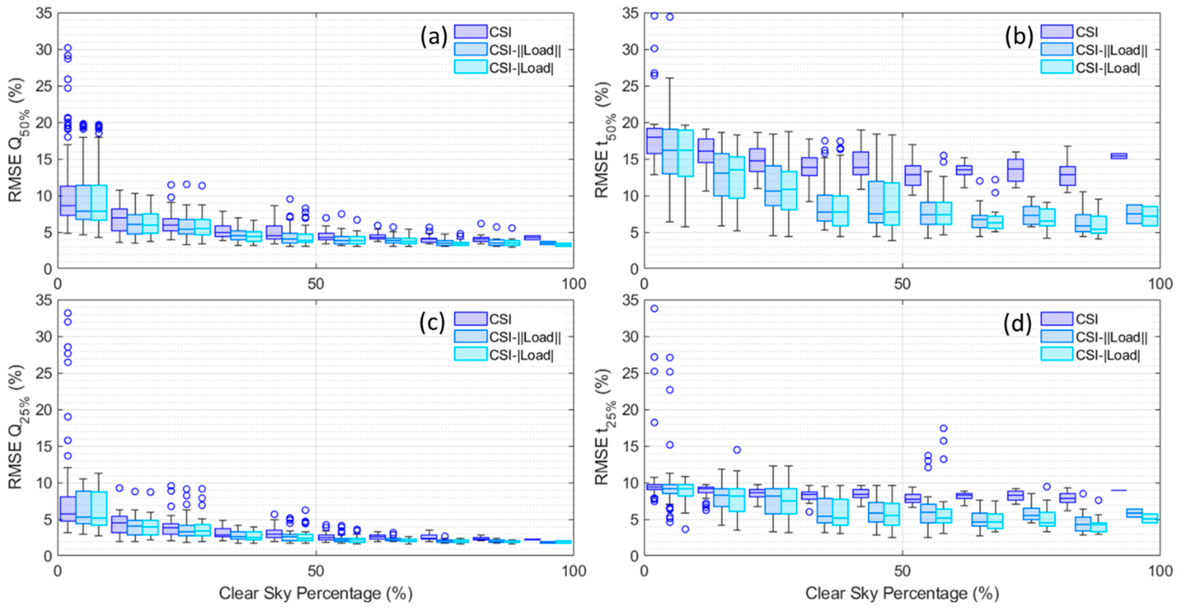
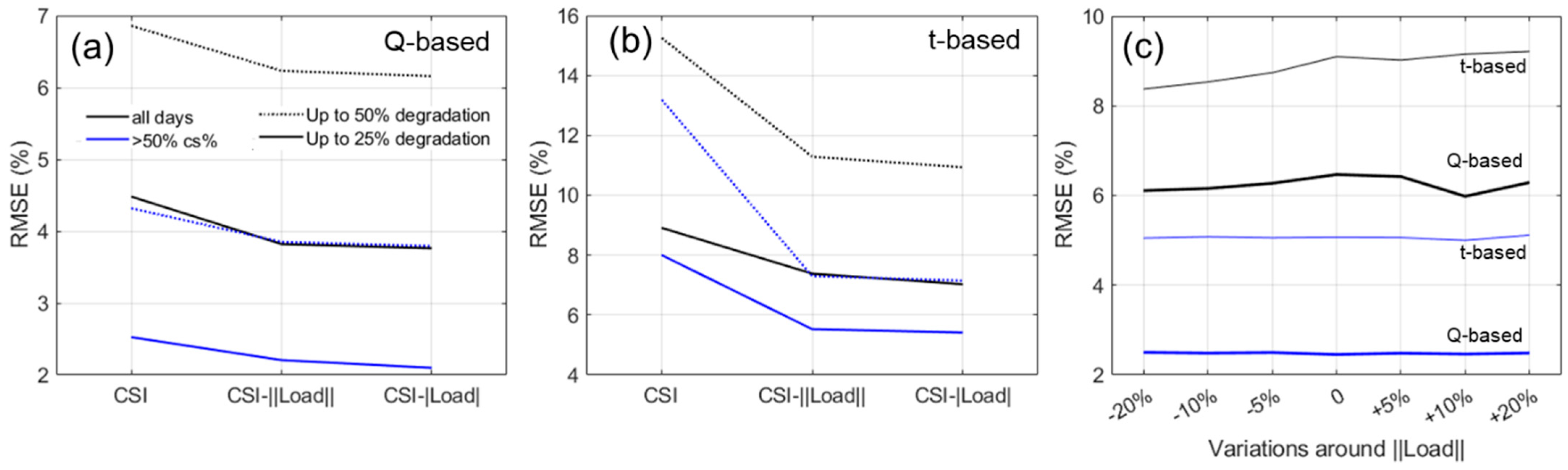
3.3. Impact of Residential Usage

Figure 4 presents the average RMSEs for the 11,000 considered degradations over 365 days as a function of the clear sky percentage in 10% increments. The results are presented as box plots where the size of the box represents 50% of the data, with the median represented by the line. The whiskers represent a 3σ deviation from the median and the circles represent the outliers. The top row presents the results for up to 50% degradation and the bottom one up to 25%. The left column shows the results from a Q-based diagnosis and the right column shows the results from a t-based one.

From a Q-based standpoint, the type of dataset used for training does not seem to have a major impact as the results are close between the CSI, CSI-|Load|, and CSI-||Load|| datasets. Nonetheless, there seems to be consistent ordering, with the RMSE for the CSI only being slightly higher than that for CSI-||Load|| and then CSI-|Load|. This ordering is much more visible when the t-based diagnosis is considered (right column), where there is a clear drop in RMSE between the CSI-trained data and the data trained with CSI minus a load, which are close but still with an advantage for CSI-|Load|.

Figure 5a,b present the evolution of the average RMSE for both the Q- and t-based diagnosis as a function of the training dataset for all days (black lines) and for days with a cs% > 50% (blue lines). Figure 5a,b confirm the observations from Figure 4 with the worst performance for the CSI-trained algorithms both for the Q- and t-based diagnosis with a bigger difference for the t-based diagnosis. The average performance for the CSI-|Load| and CSI-||Load|| is extremely similar and likely well within the margin of error for our approach. Being around 2%, this performance is also just slightly higher than the 1.75% obtained without considering additional usage [23,24]. Figure 5c displays the impact of moving the value of ||Load|| by ±20% for days with more than 50% clear sky. These variations have very little effect when days with >50 cs% are considered and only a mild effect on the t-based diagnosis when all days are considered with the lowest RMSEs for the −20% dataset.

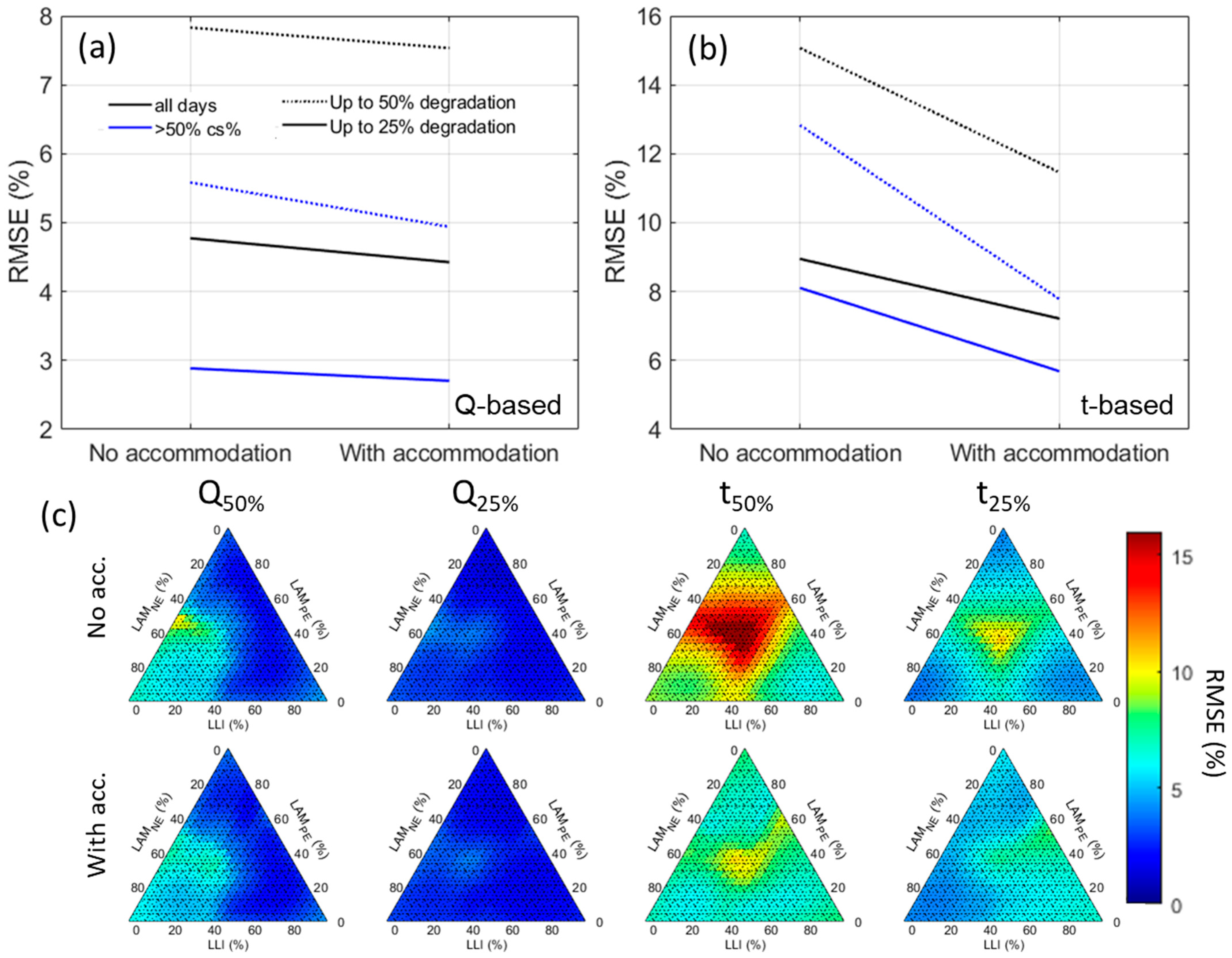
3.4. Impact of Pack Imbalance/Inhomogeneities

Figure 6a showcases the impact of increasing the RDF on the derivative of the simulated electrochemical response of the cell at C/4. More information and details on the significance of changing the RDF can be found in previous works [29,45,46]. The impact is especially visible on the local minima around 3.8 V that become progressively filled when the RDF increases by 50%. Additional effects can be seen between the low voltage and the main peak, where the two small graphitic peaks are no longer visible because of the broadening of the peaks. These voltage changes might affect the algorithm’s ability to recognize the different degradations. Figure 6b,c presents the average RMSEs associated with simulations for different levels of inhomogeneities both for the training and validation datasets. For the training datasets, the CSI dataset was used for generation with either the initial cell, the initial cell plus 25% RDF, or the initial cell plus 50% RDF. The validation dataset was generated from the OI minus the daily residential load using a cell with either 0%, 12.5%, 25%, 37.5%, or 50% increased RDF.

The error associated with an increasing RDF for the validation cycles increases for the algorithm trained on the initial cell and decreases for the algorithms trained with the initial cell plus 50% RDF. For the algorithms trained with the initial cell plus 25% RDF, a bell shape curve is observed for the Q-based diagnosis RMSEs, with a minimum for the validation data with +25% RDF. This minimum was around 1% above the homogeneous dataset average RMSEs. The bell shape is not observed for the t-based diagnosis, where the highest error was observed for lower RDFs.

4. Discussion

Looking first into the impact of additional usage on the cells, it must be noted that the HOMER-generated residential load profiles used in this work relied on empirical consumption patterns, reflecting typical household behavior. While these profiles smoothed over stochastic variations, such as those caused by individual occupant activities, we believe this approximation was suitable for the synthetic data generated in this work. Our simulations indicated only a small impact of the additional usage on the Q-based diagnosis between the unaccommodated simulations and the accommodated ones, whether by subtracting the average load or the average of the average load. Indeed, from Figure 5a, it can be seen that the average RMSE decreased by less than 1% in the all-days scenario but by less than 0.5% if only the days with 50% or more clear sky are considered, independently of the extent of the degradation. For the t-based diagnosis, the impact is much larger, especially for the larger capacity losses where 3 to 5% gain in RMSEs was calculated. As discussed in [23], the difference between the Q-based and t-based diagnosis is not surprising. Indeed, since the charge of the cells is overall rather slow, lasting more than 10 h, variations in current do not significantly impact the voltage nor the exchanged capacity, but since these variations will affect charging times, the t-based diagnosis will be affected. Since the diagnosis accuracy in the cases of training using |load|, ||load||, and ±20% around ||load|| was rather constant (Figure 5b,c), this same impact of a slow charge seems to remove the necessity of knowing the exact usage associated with each battery to be able to accommodate their effect, which is good news for applicability.

Looking into the impact of transitioning from a single-cell model to a pack model (Figure 6b,c), it appeared to be larger than that for the training datasets, with variations of more than 2% in the average RMSE reported depending on the conditions. Training on a single cell will work well for packs with little inhomogeneity but the RMSE will quickly increase with an increase in RDF, especially for Q-based diagnosis. The opposite is true when training on a model with significant inhomogeneities. The best compromise seemed to be training on a cell with mild inhomogeneities (+25% RDF in our case). In such cases, a bell-shaped curve was observed for Q-based RMSEs with less than 1% variation between the minimum and the maximum.

To investigate the impact of combining both accommodations, the last experiment consisted first of a dataset trained on the CSI without any accommodation and second a dataset trained with the CSI-||load|| with also +25% on the RDF to account for the impact of the additional usage and of inhomogeneities. The validation was performed both on a dataset using the OI minus the residential usage and a random value for the RDF increase between 0 and 50% for each day of the year. The results of these simulations are presented in Figure 7. Unsurprisingly, the t-based diagnosis benefited the most from both accommodations with an improvement in the average RMSE between 1.75 and 5.1% depending on the conditions. The improvement was much more limited for the Q-based diagnosis, where it stayed below 1%. Nonetheless, a closer investigation of the average RMSEs as a function of the type of degradation (Figure 7c) showcased some improvement, with lower RMSEs in the regions where the algorithm struggled the most. Looking at the Q-based diagnosis up to 50% (first column), and without any accommodations, the diagnosis error is the highest for degradation paths with around 50% LAM_NE (yellow area on top left triangle indicating RMSEs around 10%). After accommodation, the yellow area disappears, and the average error is much more consistent across the entire degradation paths. The same can be observed for both t-diagnosis (3rd and 4th columns), where the color distribution is much more homogeneous after accommodation, indicating an overall better performance of the algorithm. This is promising for deployment, as this indicates that the error is less dependent on the actual degradation and that, although the best diagnoses were not improved much, the worst ones were.

Overall, the accommodation of additional usage and battery packs only increased the average RMSEs for diagnosis by 1% compared to the ideal scenario (2.75% vs. 1.75% for training and validation on single cells without additional usage [23,24]). Looking to further improve the diagnosability, possible improvements could include better emulation of PV systems. In the example given, this could be accomplished by using a different model integrating maximum power point tracking [54,55]. In addition, the addition of forecasting for the global horizontal irradiance [56,57,58] could help to select the best days to perform the diagnosis. Finally, a wide variety of voltage-based diagnosis algorithms have been proposed in the literature [59,60], and some could potentially improve on the algorithm used in this work. Since this work was focused on data generation, scoping different types of algorithms was out of scope.

5. Conclusions

Following on from our previous work where we proposed a proof-of-concept approach for the diagnosis of PV-connected batteries without the need for maintenance cycles, this work addressed the two main limitations of the initial approach, where only single cells without any additional usage on the battery were considered. This work showed that, for capacity-based diagnosis, these limitations have a limited impact of the diagnosis accuracy and that they can be accommodated without adding much complexity to the approach by subtracting the average usage from the clear sky irradiance and by accounting for a medium level of inhomogeneities. These accommodations, while of limited impact for the average capacity-based diagnosis, with around a 1% increase in the average RMSE for the best-case figure, significantly improved the worst Q-based diagnoses and all the time-based diagnoses by up to 5% depending on the conditions.

Overall, this study reinforced the potential of synthetic data generation and training to enable Big-Data studies of the behavior of deployed systems experiencing sporadic usage.

References

1. Anukoolthamchote, P.C.; Assané, D.; Konan, D.E. Net electricity load profiles: Shape and variability considering customer-mix at transformers on the island of Oahu, Hawai‘i. Energy Policy 2020, 147, 111732. [Google Scholar] [CrossRef]
2. Covelli, D.; Virgüez, E.; Caldeira, K.; Lewis, N.S. Oahu as a case study for island electricity systems relying on wind and solar generation instead of imported petroleum fuels. Appl. Energy 2024, 375, 124054. [Google Scholar] [CrossRef]
3. Che, Y.; Hu, X.; Lin, X.; Guo, J.; Teodorescu, R. Health prognostics for lithium-ion batteries: Mechanisms, methods, and prospects. Energy Environ. Sci. 2023, 16, 338–371. [Google Scholar] [CrossRef]
4. Vasta, E.; Scimone, T.; Nobile, G.; Eberhardt, O.; Dugo, D.; De Benedetti, M.M.; Lanuzza, L.; Scarcella, G.; Patanè, L.; Arena, P.; et al. Models for Battery Health Assessment: A Comparative Evaluation. Energies 2023, 16, 632. [Google Scholar] [CrossRef]
5. Barrett, D.H.; Haruna, A. Artificial intelligence and machine learning for targeted energy storage solutions. Curr. Opin. Electrochem. 2020, 21, 160–166. [Google Scholar] [CrossRef]
6. Cui, Z.; Wang, L.; Li, Q.; Wang, K. A comprehensive review on the state of charge estimation for lithium-ion battery based on neural network. Int. J. Energ. Res. 2021, 46, 5423–5440. [Google Scholar] [CrossRef]
7. Sharma, P.; Bora, B.J. A Review of Modern Machine Learning Techniques in the Prediction of Remaining Useful Life of Lithium-Ion Batteries. Batteries 2022, 9, 13. [Google Scholar] [CrossRef]
8. Rauf, H.; Khalid, M.; Arshad, N. Machine learning in state of health and remaining useful life estimation: Theoretical and technological development in battery degradation modelling. Renew. Sustain. Energy Rev. 2022, 156, 111903. [Google Scholar] [CrossRef]
9. Na, H.S.; Numan-Al-Mobin, A.M. Machine learning approaches to estimate the health state of next-generation energy storage. In Green Sustainable Process for Chemical and Environmental Engineering and Science; Elsevier: Amsterdam, The Netherlands, 2023; pp. 343–363. [Google Scholar]
10. Severson, K.A.; Attia, P.M.; Jin, N.; Perkins, N.; Jiang, B.; Yang, Z.; Chen, M.H.; Aykol, M.; Herring, P.K.; Fraggedakis, D.; et al. Data-driven prediction of battery cycle life before capacity degradation. Nat. Energy 2019, 4, 383–391. [Google Scholar] [CrossRef]
11. Röder, F.; Ramasubramanian, S. A Review and Perspective on Path Dependency in Batteries. Energy Technol. 2022, 10, 2200627. [Google Scholar] [CrossRef]
12. Srinivasan, V.; Newman, J. Existence of Path-Dependence in the LiFePO4 Electrode. Electrochem. Solid-State Lett. 2006, 9, A110. [Google Scholar] [CrossRef]
13. Gering, K.L.; Sazhin, S.V.; Jamison, D.K.; Michelbacher, C.J.; Liaw, B.Y.; Dubarry, M.; Cugnet, M. Investigation of path dependence in commercial lithium-ion cells chosen for plug-in hybrid vehicle duty cycle protocols. J. Power Sources 2011, 196, 3395–3403. [Google Scholar] [CrossRef]
14. Figgener, J.; Bors, J.; Kuipers, M.; Hildenbrand, F.; Junker, M.; Koltermann, L.; Woerner, P.; Mennekes, M.; Haberschusz, D.; Kairies, K.-P.; et al. Degradation mode estimation using reconstructed open circuit voltage curves from multi-year home storage field data. ArXiv 2025, arXiv:2411.08025. [Google Scholar] [CrossRef]
15. Dubarry, M.; Berecibar, M.; Devie, A.; Anseán, D.; Omar, N.; Villarreal, I. State of health battery estimator enabling degradation diagnosis: Model and algorithm description. J. Power Sources 2017, 360, 59–69. [Google Scholar] [CrossRef]
16. Dubarry, M.; Beck, D. Analysis of Synthetic Voltage vs. Capacity Datasets for Big Data Li-ion Diagnosis and Prognosis. Energies 2021, 14, 2371. [Google Scholar] [CrossRef]
17. Dubarry, M.; Beck, D. Big data training data for artificial intelligence-based Li-ion diagnosis and prognosis. J. Power Sources 2020, 479, 228806. [Google Scholar] [CrossRef]
18. Kim, S.; Yi, Z.; Chen, B.-R.; Tanim, T.R.; Dufek, E.J. Rapid failure mode classification and quantification in batteries: A deep learning modeling framework. Energy Storage Mater. 2022, 45, 1002–1011. [Google Scholar] [CrossRef]
19. Mayilvahanan, K.S.; Takeuchi, K.J.; Takeuchi, E.S.; Marschilok, A.C.; West, A.C. Supervised Learning of Synthetic Big Data for Li-Ion Battery Degradation Diagnosis. Batter. Supercaps 2021, 5, e202100166. [Google Scholar] [CrossRef]
20. Costa, N.; Sánchez, L.; Anseán, D.; Dubarry, M. Li-ion battery degradation modes diagnosis via Convolutional Neural Networks. J. Energy Storage 2022, 55, 105558. [Google Scholar] [CrossRef]
21. Kim, S.; Jung, H.; Lee, M.; Choi, Y.Y.; Choi, J.-I. Model-free reconstruction of capacity degradation trajectory of lithium-ion batteries using early cycle data. eTransportation 2023, 17, 100243. [Google Scholar] [CrossRef]
22. Ruan, H.; Chen, J.; Ai, W.; Wu, B. Generalised diagnostic framework for rapid battery degradation quantification with deep learning. Energy AI 2022, 9, 100158. [Google Scholar] [CrossRef]
23. Dubarry, M.; Costa, N.; Matthews, D. Data-driven direct diagnosis of Li-ion batteries connected to photovoltaics. Nat. Commun. 2023, 14, 3138. [Google Scholar] [CrossRef]
24. Dubarry, M.; Yasir, F.; Costa, N.; Matthews, D. Data-Driven Diagnosis of PV-Connected Batteries: Analysis of Two Years of Observed Irradiance. Batteries 2023, 9, 395. [Google Scholar] [CrossRef]
25. Dubarry, M.; Yasir, F. Big Data for the Diagnosis and Prognosis of Deployed Energy Storage Systems. In Proceedings of the 2024 IEEE Electrical Energy Storage Application and Technologies Conference (EESAT), San Diego, CA, USA, 29–30 January 2024; pp. 1–5. [Google Scholar]
26. Li, R.; O’Kane, S.; Huang, J.; Marinescu, M.; Offer, G.J. A million cycles in a day: Enabling high-throughput computing of lithium-ion battery degradation with physics-based models. J. Power Sources 2024, 598, 234184. [Google Scholar] [CrossRef]
27. Hofmann, T.; Hamar, J.; Mager, B.; Erhard, S.; Schmidt, J.P. Transfer learning from synthetic data for open-circuit voltage curve reconstruction and state of health estimation of lithium-ion batteries from partial charging segments. Energy AI 2024, 17, 100382. [Google Scholar] [CrossRef]
28. Ruan, H.; Kirkaldy, N.; Offer, G.J.; Wu, B. Diagnosing health in composite battery electrodes with explainable deep learning and partial charging data. Energy AI 2024, 16, 100352. [Google Scholar] [CrossRef]
29. Dubarry, M.; Beck, D. Perspective on Mechanistic Modeling of Li-Ion Batteries. Acc. Mater. Res. 2022, 3, 843–853. [Google Scholar] [CrossRef]
30. Dubarry, M.; Vuillaume, N.; Liaw, B.Y. From single cell model to battery pack simulation for Li-ion batteries. J. Power Sources 2009, 186, 500–507. [Google Scholar] [CrossRef]
31. Kim, J.; Cho, B.H. Stable Configuration of a Li-Ion Series Battery Pack Based on a Screening Process for Improved Voltage/SOC Balancing. IEEE Trans. Power Electron. 2012, 17, 411–424. [Google Scholar] [CrossRef]
32. Jiang, Y.; Jiang, J.; Zhang, C.; Zhang, W.; Gao, Y.; Guo, Q. Recognition of battery aging variations for LiFePO4 batteries in 2nd use applications combining incremental capacity analysis and statistical approaches. J. Power Sources 2017, 360, 180–188. [Google Scholar] [CrossRef]
33. Tanim, T.R.; Dufek, E.J.; Sazhin, S.V. Challenges and needs for system-level electrochemical lithium-ion battery management and diagnostics. MRS Bull. 2021, 46, 420–428. [Google Scholar] [CrossRef]
34. Xu, Z.; Wang, J.; Lund, P.D.; Zhang, Y. Estimation and prediction of state of health of electric vehicle batteries using discrete incremental capacity analysis based on real driving data. Energy 2021, 225, 120160. [Google Scholar] [CrossRef]
35. Chang, L.; Wang, C.; Zhang, C.; Xiao, L.; Cui, N.; Li, H.; Qiu, J. A novel fast capacity estimation method based on current curves of parallel-connected cells for retired lithium-ion batteries in second-use applications. J. Power Sources 2020, 459, 227901. [Google Scholar] [CrossRef]
36. Krupp, A.; Ferg, E.; Schuldt, F.; Derendorf, K.; Agert, C. Incremental Capacity Analysis as a State of Health Estimation Method for Lithium-Ion Battery Modules with Series-Connected Cells. Batteries 2020, 7, 2. [Google Scholar] [CrossRef]
37. Jiang, T.; Sun, J.; Wang, T.; Tang, Y.; Chen, S.; Qiu, S.; Liu, X.; Lu, S.; Wu, X. Sorting and grouping optimization method for second-use batteries considering aging mechanism. J. Energy Storage 2021, 44, 103264. [Google Scholar] [CrossRef]
38. Wassiliadis, N.; Steinsträter, M.; Schreiber, M.; Rosner, P.; Nicoletti, L.; Schmid, F.; Ank, M.; Teichert, O.; Wildfeuer, L.; Schneider, J.; et al. Quantifying the state of the art of electric powertrains in battery electric vehicles: Range, efficiency, and lifetime from component to system level of the Volkswagen ID.3. eTransportation 2022, 12, 100167. [Google Scholar] [CrossRef]
39. Singh, A.; Lodge, A.; Li, Y.; Widanage, W.D.; Barai, A. A new method to perform Lithium-ion battery pack fault diagnostics—Part 1: Algorithm development and its performance analysis. Energy Rep. 2023, 10, 4474–4490. [Google Scholar] [CrossRef]
40. Bilfinger, P.; Rosner, P.; Schreiber, M.; Kröger, T.; Gamra, K.A.; Ank, M.; Wassiliadis, N.; Dietermann, B.; Lienkamp, M. Battery pack diagnostics for electric vehicles: Transfer of differential voltage and incremental capacity analysis from cell to vehicle level. eTransportation 2024, 22, 100356. [Google Scholar] [CrossRef]
41. Dubarry, M.; Tun, M.; Baure, G.; Matsuura, M.; Rocheleau, R.E. Battery Durability and Reliability under Electric Utility Grid Operations: Analysis of On-Site Reference Tests. Electronics 2021, 10, 1593. [Google Scholar] [CrossRef]
42. Jocher, P.; Roehrer, F.; Rehm, M.; Idrizi, T.; Himmelreich, A.; Jossen, A. Scaling from cell to system: Comparing Lithium-ion and Sodium-ion technologies regarding inhomogeneous resistance and temperature in parallel configuration by sensitivity factors. J. Energy Storage 2024, 98, 112931. [Google Scholar] [CrossRef]
43. Rosenberger, N.; Rosner, P.; Bilfinger, P.; Schöberl, J.; Teichert, O.; Schneider, J.; Abo Gamra, K.; Allgäuer, C.; Dietermann, B.; Schreiber, M.; et al. Quantifying the State of the Art of Electric Powertrains in Battery Electric Vehicles: Comprehensive Analysis of the Tesla Model 3 on the Vehicle Level. World Electr. Veh. J. 2024, 15, 268. [Google Scholar] [CrossRef]
44. Dubarry, M.; Beck, D. Investigation of the impact of different electrode inhomogeneities on the voltage response of Li-ion batteries. Cell Rep. Phys. Sci. 2024, 102138, in press. [Google Scholar] [CrossRef]
45. Dubarry, M.; Truchot, C.; Liaw, B.Y. Synthesize battery degradation modes via a diagnostic and prognostic model. J. Power Sources 2012, 219, 204–216. [Google Scholar] [CrossRef]
46. Schindler, S.; Baure, G.; Danzer, M.A.; Dubarry, M. Kinetics accommodation in Li-ion mechanistic modeling. J. Power Sources 2019, 440, 227117. [Google Scholar] [CrossRef]
47. Ineichen, P.; Perez, R. A new airmass independent formulation for the Linke turbidity coefficient. Sol. Energy 2002, 73, 151–157. [Google Scholar] [CrossRef]
48. Liu, B.Y.H.; Jordan, R.C. The interrelationship and characteristic distribution of direct, diffuse and total solar radiation. Sol. Energy 1960, 4, 1–19. [Google Scholar] [CrossRef]
49. Loutzenhiser, P.G.; Manz, H.; Felsmann, C.; Strachan, P.A.; Frank, T.; Maxwell, G.M. Empirical validation of models to compute solar irradiance on inclined surfaces for building energy simulation. Sol. Energy 2007, 81, 254–267. [Google Scholar] [CrossRef]
50. HNEI. Alawa Central. Available online: https://www.hnei.hawaii.edu/alawa (accessed on 13 April 2025).
51. Sieg, J.; Storch, M.; Fath, J.; Nuhic, A.; Bandlow, J.; Spier, B.; Sauer, D.U. Local degradation and differential voltage analysis of aged lithium-ion pouch cells. J. Energy Storage 2020, 30, 101582. [Google Scholar] [CrossRef]
52. Devie, A.; Dubarry, M. Durability and Reliability of Electric Vehicle Batteries under Electric Utility Grid Operations. Part 1: Cell-to-Cell Variations and Preliminary Testing. Batteries 2016, 2, 28. [Google Scholar] [CrossRef]
53. Abadi, M.; Barham, P.; Chen, J.; Chen, Z.; Davis, A.; Dean, J.; Devin, M.; Ghemawat, S.; Irving, G.; Isard, M.; et al. TensorFlow: A system for large-scale machine learning. In Proceedings of the 12th USENIX Symposium on Operating Systems Design and Implementation (OSDI ‘16), Savannah, GA, USA, 2–4 November 2016. [Google Scholar]
54. Harrison, A.; Alombah, N.H.; Kamel, S.; Kotb, H.; Ghoneim, S.S.M.; El Myasse, I. A Novel MPPT-Based Solar Irradiance Estimator: Integration of a Hybrid Incremental Conductance Integral Backstepping Algorithm for PV Systems with Experimental Validation. Eng. Proc. 2023, 56, 262. [Google Scholar] [CrossRef]
55. Harrison, A.; Alombah, N.H.; Kamel, S.; Ghoneim, S.S.M.; El Myasse, I.; Kotb, H. Towards a Simple and Efficient Implementation of Solar Photovoltaic Emulator: An Explicit PV Model Based Approach. Eng. Proc. 2023, 56, 261. [Google Scholar] [CrossRef]
56. Elmousaid, R.; Drioui, N.; Elgouri, R.; Agueny, H.; Adnani, Y. Accurate short-term GHI forecasting using a novel temporal convolutional network model. e-Prime Adv. Electr. Eng. Electron. Energy 2024, 9, 100667. [Google Scholar] [CrossRef]
57. Qin, C.; Srivastava, A.K.; Saber, A.Y.; Matthews, D.; Davies, K. Geometric Deep-Learning-Based Spatiotemporal Forecasting for Inverter-Based Solar Power. IEEE Syst. J. 2023, 17, 3425–3435. [Google Scholar] [CrossRef]
58. Matthews, D.K. Determination of broadband atmospheric turbidity from global irradiance or photovoltaic power data using deep neural nets. Energy AI 2023, 14, 100252. [Google Scholar] [CrossRef]
59. Vanem, E.; Wang, S. Data-driven state of health and state of safety estimation for alternative battery chemistries—A comparative review focusing on sodium-ion and LFP lithium-ion batteries. Future Batter. 2025, 5, 100033. [Google Scholar] [CrossRef]
60. De la Iglesia, D.H.; Corbacho, C.C.; Dib, J.Z.; Alonso-Secades, V.; López Rivero, A.J. Advanced Machine Learning and Deep Learning Approaches for Estimating the Remaining Life of EV Batteries—A Review. Batteries 2025, 11, 17. [Google Scholar] [CrossRef]
Figure 1. Schematic representation of the dataset generated in this work to assess the impact of additional residential usage with (a) an example of the observed irradiance for four days within the one-year dataset. (b) The calculated clear sky irradiance of one randomly selected day, for which (c) presents the observed irradiance. (d) The simulated daily residential power usage for one year, with (e) presenting the average value and (f) the average of the average along with ±20% variations. (gi) Illustrates the three different training datasets and (j) the one used for validation.
Batteries 11 00154 g001
Figure 2. (a) Distribution of the observed vs. clear sky mean irradiances through 2017 and (b) associated clear sky percentages.
Batteries 11 00154 g002
Figure 3. (a) Example of the residential load simulations for 1 January 2017, showcasing the mix of origins for required power between the PV system, the grid, and the battery. (b) Comparison of the power generated from the clear sky irradiance, the observed irradiance, and the one used to charge the battery on 1 January with or without adjustments to accommodate additional loads. (c) Variability of the simulated residential load as a function of the day of the year with (d) the associated average usage, and the average of the average usage ± 20%.
Batteries 11 00154 g003
Figure 4. Evolution of the RMSE for diagnosis for (a) up to 50% capacity loss based on capacity, (b) up to 50% capacity loss based on time, (c) up to 25% capacity loss based on capacity, and (d) up to 50% capacity loss based on time.
Batteries 11 00154 g004
Figure 5. Effect of the training dataset on the average RMSE for (a) the Q-based diagnosis and (b) the t-based diagnosis. (c) Effect of variations around ||Load|| on the average RMSE.
Batteries 11 00154 g005
Figure 6. (a) Effect of increasing the RDF on the cell electrochemical response. Effect of the amount of inhomogeneities on the average RMSE for (b) the Q-based diagnosis and (c) the t-based diagnosis.
Batteries 11 00154 g006
Figure 7. Effect of the accommodation on the average RMSE for (a) the Q-based diagnosis and (b) the t-based diagnosis. (c) Diagnosis accuracy for days with >50% cs% as a function of the degradation path for simulation without accommodation (top row) and with accommodation (bottom row).
Batteries 11 00154 g007
Disclaimer/Publisher’s Note: The statements, opinions and data contained in all publications are solely those of the individual author(s) and contributor(s) and not of MDPI and/or the editor(s). MDPI and/or the editor(s) disclaim responsibility for any injury to people or property resulting from any ideas, methods, instructions or products referred to in the content.