A Regression-Based Technique for Capacity Estimation of Lithium-Ion Batteries

Abstract

Electric vehicles (EVs) and hybrid vehicles (HEVs) are being increasingly utilized for various reasons. The main reasons for their implementation are that they consume less or do not consume fossil fuel (no carbon dioxide pollution) and do not cause sound pollution. However, this technology has some challenges, including complex and troublesome accurate state of health estimation, which is affected by different factors. According to the increase in electric and hybrid vehicles’ application, it is crucial to have a more accurate and reliable estimation of state of charge (SOC) and state of health (SOH) in different environmental conditions. This allows improving battery management system operation for optimal utilization of a battery pack in various operating conditions. This article proposes an approach to estimate battery capacity based on two parameters. First, a practical and straightforward method is introduced to assess the battery’s internal resistance, which is directly related to the battery’s remaining useful life. Second, the different least square algorithm is explored. Finally, a promising, practical, simple, accurate, and reliable technique is proposed to estimate battery capacity appropriately. The root mean square percentage error and the mean absolute percentage error of the proposed methods were calculated and were less than 0.02%. It was concluded the geometry method has all the advantages of a recursive manner, including a fading memory, a close form of a solution, and being applicable in embedded systems.

1. Introduction

The availability of new energy sources to different countries is fundamental for their economic development [1]. It is well known that petrol and diesel fuel vehicles lead to a significant amount of greenhouse gasses such as CO₂, which has severe and dangerous effects on the environment cause global warming [2]. Currently, lithium-ion batteries for electric vehicles (EVs) and hybrid electric vehicles (HEVs) are the most promising propulsion alternative to internal combustion engines (ICEs) due to not producing carbon dioxide and sound pollution. Thus, in the not-too-distant future, we will essentially see the replacement of many ICE vehicles with EVs and HEs and this replacement process has already started. The central part of these vehicles is a rechargeable battery that must have reasonable and acceptable efficiency [3]. Lithium-ion batteries have many benefits in comparison to other types of batteries, such as higher energy capacity, longer functional life, and less self-discharge in comparison with different kinds of rechargeable batteries, such as Ni-Cd batteries, which makes them attractive for many different applications, such as portable electronic devices, electric vehicles, and stationary storage [4,5]. Therefore, this battery is attracting the attention of the electric vehicle industry [5].

A lithium-ion battery pack consists of a considerable number of battery cells, which are connected in series and parallel. Despite the above-mentioned advantages, there are also some challenges, such as costs, cycling stability, and safe operation. Parameters such as charge and discharge rate, temperature, and voltage range will influence the safety of the battery. If critical limits of these parameters are exceeded, this will accelerate the degradation, and thus reduce the battery performance, and may even become dangerous due to the increased risk of a thermal runaway.

Furthermore, it is crucial to have an exact measurement of lithium-ion battery total capacity and to provide the ability to predict the remaining useful life (RUL) over the entire service duration in order to ensure the trusted and safe operation of these batteries [6]. This RUL prediction ability represents an essential part of the battery management system (BMS), which is needed to keep the battery operational in a safe, trusted, and reliable state under all conditions. This unit includes complex electronic circuitry and dedicated algorithms, which control the battery function [7].

Batteries age through regular use and during storage and transport with (simultaneous) exposure to temperature. For example, changes in the crystal chemistry of the active materials occur due to frequent cycling combined with cracking of the particles and formation of a new solid-state electrolyte interface SEI (consumption of electrolyte and lithium). Two parameters show the ageing status of a battery. The first is the battery’s total capacity, which is given by $Q$, and the second is equivalent internal resistance $R_e$. When $Q$ has decreased to 80% of the initial (or nominal) capacity in an electric car, it is recommended to replace the battery because it cannot satisfy the high requirements for such applications. However, it could still be used in a second life application. Such an application could be, e.g., a stationary battery for peak shaving, which needs a lower depth of discharge (DOD) and less power. Similarly, if $R_e$ grows to 160% of its initial value, the battery in an EV needs to be replaced as well [8,9].

The state of health (SOH) is defined as the ratio of the currently measured maximum battery charge to its nominal capacity. The following equation shows how the SOH parameter is expressed as a percentage:

$$SOH=\frac{Q_{act}}{Q_{nom}}\ast 100$$

(1)

in which $Q_{act}$ and $Q_{nom}$ are the total capacity and the nominal capacity, respectively [9].

The most general and common method, which is used in the laboratory to estimate SOH, is coulomb counting (CC). At first, the fully charged battery is discharged to the 0% state of charge defined by the manufacturer in particular conditions, and the whole ampere-hour, which is discharged, is being measured. Then SOH is calculated by dividing discharged ampere-hour value by the initial capacity [10]. As mentioned above, this method is only used to collect data in the laboratory. Existing capacity estimation methods and SOH estimation could be categorized into three groups.

The first group includes the physics-based methods that use partial differential equations to model battery electrochemical properties and thermal behavior. Even though these methods have high accuracy, they are not suitable for online use because of the high calculation load [11].

The second group includes data-driven models that estimate battery capacity by analyzing such characteristics as voltage and extracting some unique features. This method is strongly correlated to battery ageing without any mathematical model. In the ICA method, for instance, the IC curve is obtained by the following equation:

$$IC=\frac{dQ}{dV}\approx \frac{\Delta Q}{\Delta V}$$

(2)

Plateaus observed in the voltage curve are transformed to characteristics as identifiable peaks. Some particular features of these peaks, such as height, area, and position, are directly related to battery capacity and make the battery state of health estimation simple [12]. Differential voltage analysis (DVA) is another method of this group. The differential voltage (DV) curve is defined as voltage gradient divided by actual capacity:

$$\frac{dV}{dQ}=\frac{dV}{{\displaystyle \int Idt}}=\frac{dV}{Idt}$$

(3)

Then SOH is analytically calculated by making a relationship between DV and SO. characteristics [13]. However, despite their advantages, these methods face fundamental challenges that limit their application. For example, IC and DV curves are subjected to noise and should be smoothed before using for estimation. The smoothing process needs some computational effort. Temperature variation affects their accuracy and makes capacity prediction infected with error. In addition, charging and discharging characteristics used to extract IC and DV curves are different from the actual usage profile. Other data-driven methods exist that use algorithms such as fuzzy logic and neural network. Experimental data of complicated and nonlinear systems can be processed by a fuzzy rule set of the fuzzy logic (FL) method. There are two sets of data: crisp and fuzzy. When data are divided by definite values, they belong to a crisp group, and if they are categorized by uncertainty, they belong to the fuzzy group. Membership functions determine members of fuzzy sets. The more the appropriate membership function is defined, the better prediction of SOH will be obtained [14,15]. In [15], a relationship between several cycles and the normalized value of battery capacity is received by an exponential curve-fitting on NASA data as follows:

$$y_{fit}=a_0+a_1{e}^{-\left(\frac{x}{{\alpha }_1}\right){\beta }_1}+a_2{e}^{-\left(\frac{x}{{\alpha }_2}\right){\beta }_2}$$

(4)

It uses the local estimation form of $y=a{e}^{-\beta x}$ to reduce the number of parameters. Then it applies the impact of parameters such as temperature, current, and DOD by three membership functions of fuzzy logic that modify $a$ and $\beta$ factors. A disadvantage of this model is that a significant number of data are needed to define membership functions, and thus, many laboratory tests are necessary to obtain enough data in particular operating conditions. A neural network (NN) is a powerful tool that can manage a significant amount of data in a highly complex nonlinear system. One of the advantages of a NN is that it is not necessary to have detailed knowledge about battery characteristics. A robust algorithm that can accurately predict SOH in different working conditions is another benefit of NN [16]. High computational load and cost are the main obstacles in implementing the NN algorithm. Another limitation to obtaining accurate answers is data training that must work with a considerable amount of different data [17]. Sample entropy (SE) is a method that records oscillation, instability, and complication of the battery’s voltage response in capacity fade duration. Therefore, it is a kind of diagnostic tool that can record battery capacity. This method commonly uses other ways to have more accurate results [18].

The third group is empirical-based methods that describe battery behavior by employing phenomenological elements such as equivalent circuit models (ECM). The accuracy of these strategies is not as high as physics-based methods, but the computational load is much lower. In addition, empirically based approaches do not face the aforementioned challenges of the data-driven process. An example of these kinds of models is the impedance spectroscopy method that estimates SOH using a broad frequency spectrum. Computing equivalent circuit model parameters make estimation easier [19].

Algorithms and filters are used to achieve faster and more accurate results. Kalman Filter (KF) is a powerful algorithm that can precisely estimate SOH parameters. For nonlinear systems, the KF is more reasonable. In addition, nonlinear systems use some modified types of this algorithm, such as dual extended Kalman filter (DEKF) and unscented Kalman filter (UKF) [20]. Particle filter (PF) uses sampling and resampling (Sequential Monte Carlo) algorithm, and a collection of weighted particles to solve filtering problems is used to estimate the probability density function (PDF) [21].

The main factor determining whether electric vehicles (EVs) earn their place in daily applications is batteries lifetime. Choosing a mathematical model that models the physical dynamics and constraints of a battery with high precision is crucial to increase estimation accuracy. Therefore, the chosen model should be able to cover errors from uncontrollable working conditions, sensor inaccuracies, and other noise sources to enable an accurate estimation. This paper used an ECM of the battery, which gave the relationship between SOC and the total capacity $Q$. In addition, the SOC data were obtained by providing voltage and current data as input to this model. Then, this relationship was rearranged to a form of $y=Qx$ that made it possible to estimate $Q$ by the regression (least squares) method. Different forms of the least-squares method are proposed in this article, and the results are compared.

The main contributions of the proposed methods are as follow:

• Current measurement error and SOC estimation error are considered in the proposed method.
• The proposed methods are closed-form and recursive. This means they do not need high computational effort and high memory space.
• In addition, a proposed method is fading memory. This gives weight to recent data and fades the effect of early data. This makes proposed methods applicable in online applications and increases capacity estimation during several cycles for SOH estimation.

The following three sections of the article provide some reasons for the ageing of lithium-ion batteries, describe the capacity estimation method, and show the validation of the model using experimental data. In the end, some conclusions are given.

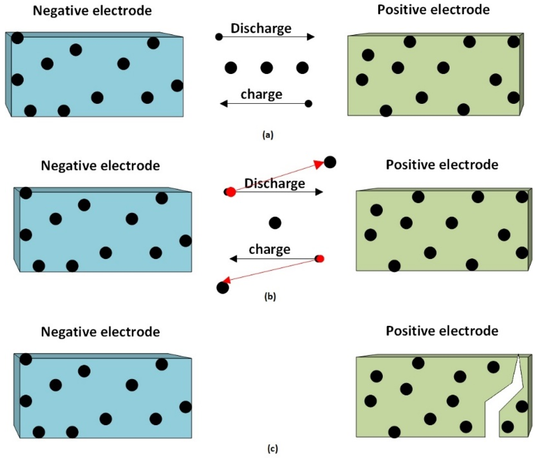
2. Reasons for Lithium-Ion Batteries Ageing

Capacity decrease and power fade of lithium-ion batteries are complicated phenomena that originated for various reasons. Processes influence the calendar life of the battery during storage, such as impedance rise and self-discharge. Whereas ageing processes occur during use, such as lithium metal plating, mechanical degradation affects cycle life. It should be considered that ageing processes with cycle life and calendar life originated from changes of:

• Interface of electrolyte and electrodes;
• Active material;
• Composite electrode.

A straightforward model of electrodes is shown in Figure 1. Battery power results from ion transition between electrodes. The power will decay if this transition is disrupted or damaged. Side reactions include structural decay and are the main cause of disruption of the ion current [22,23].

This phenomenon degrades lithium-ion batteries over time and changes their parameters. It is well established that SEI growth and lithium plating are essential ageing mechanisms in modern lithium batteries. Therefore, it is necessary to estimate ageing parameters and adjust some of them to manage battery packs. These estimations algorithms are part of the BMS unit.

One of the approaches to evaluate lithium-ion battery ageing is to model its behavior by electrical elements, known as equivalent circuit model. This is a prevalent method due to a tradeoff between accuracy in open-circuit voltage estimation and computational load [24,25,26,27]. The equivalent circuit method is shown in Figure 2, and our approach to estimating SOC is to calculate the value of equivalent-series resistance and total capacity. Both side reaction and structural decay will reduce the lithium-ion storage capability in one or both electrodes, reducing total capacity, known as capacity fade. The cell’s series resistance will increase with ageing and result in power fade. Some ageing mechanisms, such as structural decay and SEI growth, could happen even in the rest time of the battery.

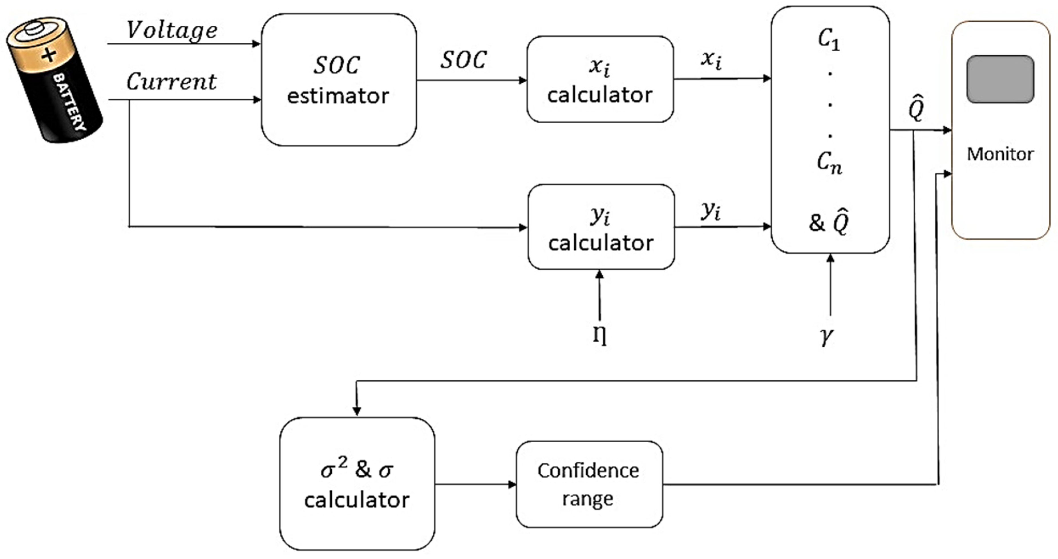
3. Capacity Estimation

3.1. Calculation of $R_0$

The equivalent circuit model for the battery is shown in Figure 2; the relationship between circuit parameters are given by the following equation:

$$v_{b,k}=OCV\left(SO{C}_k\right)+M{h}_k-{\displaystyle \sum }_i{R}_i{i}_{R_{i,k}}-i_{b,k}{R}_e$$

(5)

In the above equation, $v_{b,k}$ and $i_{b,k}$ are the battery voltage and current, $OCV\left(SO{C}_k\right)$ is the open-circuit voltage that is a function of state of charge, $M{h}_k$ is hysteresis voltage, $R_i{i}_{R_{i,k}}$ is the multiple of $i^{th}$ resistance of capacitor-resistance nets in the corresponding current, and $i_{b,k}{R}_e$ is the multiple of series resistance in the battery current.

If we define $S_{vb}^{Re}$ as the sensitivity of voltage to rate of change in resistance $R_e$, we have:

$$S_{v_{b,k}}^{R_e}=\frac{R_e}{v_{b,k}} \frac{d{v}_{b,k}}{d{R}_e}=\frac{-R_e}{v_{b,k}} i_{b,k}$$

(6)

The equation shows that bigger $i_{b,k}$ leads to higher sensitivity to changes in $R_e$. In this part a method is described for estimating of $R_e$ by subtracting $v_{b,k}$ of two adjacent samples:

$$\begin{array}{c}{v}_{b,k}=OCV\left(SO{C}_k\right)+M{h}_k-{\displaystyle \sum }_i{R}_i{i}_{R_{i,k}}-i_{b,k}{R}_e\hfill \\ v_{b,k-1}=OCV\left(SO{C}_{k-1}\right)+M{h}_{k-1}-{\displaystyle \sum }_i{R}_i{i}_{R_{i,k-1}}-i_{b,k-1}{R}_e\hfill \\ \_\_\_\_\_\_\_\_\_\_\_\_\_\_\_\_\_\_\_\_\_\_\_\_\_\_\_\_\hfill \\ v_{b,k}-v_{b,k-1}=R_e\left(i_{b,k-1}-i_{b,k}\right)\hfill \end{array}$$

(7)

As can be seen, the rate of change in $R_e$ is impressively bigger than other variables in the equation:

$${\widehat{R}}_{e,k}=\frac{v_{b,k}-v_{b,k-1}}{i_{b,k-1}-i_{b,k}}$$

(8)

where ${\widehat{R}}_{e,k}$ is the estimated and not exact value of $R_{e,k}$. It should be considered that ${\widehat{R}}_e$ could be estimated only when $\Delta i_{b,k}\ne 0$. In this regard, a minimum limit value has been considered in the simulation as the threshold in order to not consider minimal values of $\Delta i_{b,k}$. Therefore, using a filter simply can reduce the error:

$${\widehat{R}}_{e,k}^{filt}=\alpha {\widehat{R}}_{e,k-1}^{filt}+\left(1-\alpha \right){\widehat{R}}_{e,k}$$

(9)

where $0\ll \alpha <1$. The equivalent series resistance is SOC-dependent and temperature-dependent. By defining a vector of $R_e$ in different SOC levels, the first problem will be solved, and by adopting a matrix of resistance for various temperature and SOC levels, both will be solved.

3.2. Proposed Methods to Estimate $Q$

Here we define a parameter that shows voltage variation proportional to capacity, similar to the last part:

$$S_{v_{b,k}}^Q=\frac{Q}{v_{b,k}} \frac{d{v}_{b,k}}{dQ}=\frac{Q}{v_{b,k}} \frac{d}{dQ} \left(ocv \left(so{c}_k\right)+M{h}_k-{{\displaystyle \sum }}_i{R}_i{i}_{R_{i,k}}-i_{b,k}{R}_e\right)$$

(10)

The derivative of components in parenthesis was computed as the following equation:

$$\frac{dOCV}{dQ}=\frac{\partial OCV\left(SO{C}_k\right)}{\partial SO{C}_k} \frac{dSO{C}_k}{dQ}$$

(11)

In most battery cells, $\frac{\partial OCV\left(SO{C}_k\right)}{\partial SO{C}_k}$ is very small. The equation which was derived from SOC relationships can be rewritten as the following equation:

$$SOC\left[k+1\right]=SOC\left[k\right]-\frac{\eta \left[k\right]\Delta t}{Q}{i}_b\left[k\right]$$

(12)

In which $SOC\left[k\right]$ is state of charge, $\eta \left[k\right]$ is columbic efficiency, which shows the consumer will not receive the whole charge stored in the battery due to some unwanted side reactions. In addition, a tiny part of it is being lost. Usually, this parameter is very near to one. $\Delta t$ is sampling time for discretization, $i_b\left[k\right]$ is battery current, and $Q$ is the total capacity of the battery.

It can be derived from the following equation that the sensitivity of voltage to capacity through hysteresis term is minor and zero through other terms. So total capacity is not observable [28].

$$\begin{array}{cc}\frac{dSOC\left[k\right]}{dQ}& =\frac{dSOC\left[k-1\right]}{dQ}-\eta \left[k-1\right]i_b\left[k-1\right]\Delta t\frac{d\frac{1}{Q}}{dQ} \hfill \\ & =\frac{dSOC\left[k-1\right]}{dQ}+\frac{\eta \left[k-1\right]i_b\left[k-1\right]\Delta t}{Q^2}\hfill \end{array}$$

(13)

It can be seen from the above equation that $\frac{dSOC\left[k\right]}{dQ}$ increases while the direction of $i_b\left[k\right]$ does not change in a considerable period. This is because of $\Delta t$ (by order of 1/3600 or less).

In this part, a procedure is described to analyze some possible methods of estimating $Q$ and their disadvantages. Finally, an approach is proposed to have an accurate, robust estimate of $Q$.

Considering Equation (13), we have:

$$SOC\left[k_n\right]=SOC\left[k_1\right]-\frac{\Delta t}{Q}{\displaystyle \sum }_{k_1}^{k_{n-1}}\eta \left[k\right]i_b\left[k\right]$$

(14)

The above equation could be rewritten as:

$$-\Delta t {\displaystyle \sum }_{k_1}^{k_{n-1}}\eta \left[k\right]i_b\left[k\right]=Q\left(SOC\left[k_n\right]-SOC\left[k_1\right]\right)$$

(15)

By defining $Y=-\Delta t {\displaystyle \sum _{k_1}^{k_{n-1}}}\eta \left[k\right]i_b\left[k\right]$ and $X=SOC\left[k_n\right]-SOC\left[k_1\right]$, it could be written in a linear format: $Y=QX$.

3.2.1. The First Type of Least Squares Method

The standard (weighted least squares) linear regression is the first investigated method to solve the above equation. By considering $\Delta y$ as the noise on measurement and uncertainties of $y$, the form of the problem is:

$$\left(y-\Delta y\right)=Qx$$

(16)

In the above equation, $\Delta y$ includes zero-mean Gaussian random variables with variances of ${\sigma }_{y_i}^2$. The estimated $Q$ could be shown by $\widehat{Q}$, then $y\approx \widehat{Q}x$, can be solved by using vectors of measured data of $x$ and $y$:

$$x_i=SOC\left[k_{2,i}\right]-SOC\left[k_{1,i}\right]$$

(17)

$$y_i=-\Delta t {\displaystyle \sum }_{k_{1,i}}^{k_{2,i}-1}\eta \left[k\right]i_b\left[k\right]$$

(18)

In this level, the $\widehat{Q}$ is estimated which minimizes the following first type of least-squares (LS1) cost function:

$${\chi }_{LS1}^2={\displaystyle \sum }_{i=1}^n\frac{{\left(y_i-Y_i\right)}^2}{{\sigma }_{y_i}^2 }={\displaystyle \sum }_{i=1}^n\frac{{\left(y_i-\widehat{Q}{x}_i\right)}^2}{{\sigma }_{y_i}^2 }$$

(19)

In which $Y_i$ is the exact value of $Y$ without noise ($Y_i=\widehat{Q}{x}_i$). By differentiating the above cost function concerning $\widehat{Q}$ and setting it to zero, the following equations could be determined:

$$\frac{\partial {\chi }_{LS1}^2}{\partial \widehat{Q}}=-2 {\displaystyle \sum }_{i=1}^N\frac{x_i\left(y_i-\widehat{Q}{x}_i\right)}{{\sigma }_{y_i}^2}=0$$

(20)

$$\widehat{Q} {\displaystyle \sum }_{i=1}^N\frac{x_i{}^2}{{\sigma }_{y_i}^2}={\displaystyle \sum }_{i=1}^N\frac{x_i{y}_i}{{\sigma }_{y_i}^2}$$

(21)

$$\widehat{Q}={\displaystyle \sum }_{i=1}^N\frac{x_i{y}_i}{{\sigma }_{y_i}^2} /{\displaystyle \sum }_{i=1}^N\frac{x_i{}^2}{{\sigma }_{y_i}^2}$$

(22)

By defining $C_1={\displaystyle \sum _{i=1}^N}\frac{x_i{}^2}{{\sigma }_{y_i}^2}$ and $C_2={\displaystyle \sum _{i=1}^N}\frac{x_i{y}_i}{{\sigma }_{y_i}^2}$, the following statement can be derived:

$$\widehat{Q}=\frac{C_2}{C_1}$$

(23)

$C_1$ and $C_2$ could be updated recursively by the following equations. Those as mentioned above could be determined when each new ($x_i$,$y_i$) datum is received:

$$C_{1,n}={\displaystyle \sum }_{i=1}^N\frac{x_i{}^2}{{\sigma }_{y_i}^2}=C_{1,n-1}+\frac{x_n^2}{{\sigma }_{y_n}^2}$$

(24)

$$C_{2,n}={\displaystyle \sum }_{i=1}^N\frac{x_i{y}_i}{{\sigma }_{y_i}^2}=C_{2,n-1}+\frac{x_n{y}_n}{{\sigma }_{y_n}^2}$$

(25)

$${\widehat{Q}}_n=\frac{C_{2,n}}{C_{1,n}}$$

(26)

Minimum storage requirement and computational load are advantages of the recursive manner in equations, and it is essential for implementing in BMS and other embedded units.

By increasing the number of data pairs, data volumes are weighted, and new data pairs cannot significantly affect the results. Therefore, there is a need to change the method to fade older data pairs’ power on results as the number of data pairs increases. Therefore, a coefficient such as $0\ll \gamma <1$ can solve this issue:

$${\tilde{C}}_{1,n}={\displaystyle \sum }_{i=1}^n{\gamma }^{n-i}\frac{x_i{}^2}{{\sigma }_{y_i}^2}=\gamma {\tilde{C}}_{1,n-1}+\frac{x_n^2}{{\sigma }_{y_n}^2}$$

(27)

$${\tilde{C}}_{2,n}={\displaystyle \sum }_{i=1}^n{\gamma }^{n-i}\frac{x_i{y}_i}{{\sigma }_{y_i}^2}=\gamma {\tilde{C}}_{2,n-1}+\frac{x_n{y}_n}{{\sigma }_{y_n}^2}$$

(28)

This method (LS1) could be an acceptable method if there were no measurement noise or uncertainty of $x_i$, but in reality, the error in SOC estimation will never be totally eliminated. The solution could be the second type of least squares.

3.2.2. The Second Type of Least Squares Method

By considering noise of $x_i$, the linear form of the problem changes as:

$$y-\Delta y=Q \left(x-\Delta x\right)$$

(29)

where $\Delta y$ and $\Delta x$ are white noise with zero mean and known variances of ${\sigma }_{y_i}^2$ and ${\sigma }_{x_i}^2$. The cost function is rewritten as:

$${\chi }_{LS2}^2={\displaystyle \sum }_{i=1}^n\frac{{\left(x_i-X_i\right)}^2}{{\sigma }_{x_i}^2 }+\frac{{\left(y_i-Y_i\right)}^2}{{\sigma }_{y_i}^2 }-{\lambda }_i\left(Y_i-\widehat{Q}{X}_i\right)$$

(30)

In which the last term applies constraint of $Y_i=\widehat{Q}{X}_i$ with Lagrange multipliers of ${\lambda }_i$.

By differentiating cost functions with respect to $X_i$, $Y_i$, and ${\lambda }_i$, setting them to zero, and placing the results in the cost function, new equations can be derived. The function with known and straightforward terms can be reached by employing the following equations:

$$\frac{\partial {\chi }_{LS2}^2}{\partial {\lambda }_i}=-\left(Y_i-\widehat{Q}{X}_i\right)=0\to {\mathit{Y}}_{\mathit{i}}=\widehat{\mathit{Q}}{\mathit{X}}_{\mathit{i}}$$

(31)

$$\frac{\partial {\chi }_{LS2}^2}{\partial Y_i}=\frac{-2\left(y_i-Y_i\right)}{{\sigma }_{y_i}^2}-{\lambda }_i=0\to {\mathit{\lambda }}_{\mathit{i}}=\frac{-2 \left({\mathit{y}}_{\mathit{i}}-{\mathit{Y}}_{\mathit{i}}\right)}{{\mathit{\sigma }}_{{\mathit{y}}_{\mathit{i}}}^2}$$

(32)

$$\frac{\partial {\chi }_{LS2}^2}{\partial X_i}=\frac{-2\left(x_i-X_i\right)}{{\sigma }_{x_i}^2}+{\lambda }_i\widehat{Q}=0=-\frac{2\left(x_i-X_i\right)}{{\sigma }_{x_i}^2}-\frac{2\left(y_i-Y_i\right)}{{\sigma }_{y_i}^2}\widehat{Q}$$

(33)

$${\sigma }_{y_i}^2 \left(x_i-X_i\right)+{\sigma }_{x_i}^2 \left(y_i-Y_i\right)\widehat{Q}={\sigma }_{y_i}^2{x}_i-{\sigma }_{y_i}^2{X}_i+{\sigma }_{x_i}^2{y}_i\widehat{Q}-{\sigma }_{x_i}^2{X}_i{\widehat{Q}}^2$$

(34)

$$X_i=\frac{{\sigma }_{y_i}^2{x}_i+{\sigma }_{x_i}^2{y}_i\widehat{Q}}{{\sigma }_{y_i}^2+{\sigma }_{x_i}^2{\widehat{Q}}^2}$$

(35)

By replacing these quantities in cost function:

$$\begin{array}{cc}{\chi }_{LS2}^2& ={\displaystyle \sum _{i=1}^N}\frac{{\widehat{Q}}^2{\sigma }_{x_i}^4{\left(y_i-\widehat{Q}{x}_i\right)}^2}{{\sigma }_{x_i}^2{\left({\sigma }_{y_i}^2+{\widehat{Q}}^2{\sigma }_{x_i}^2\right)}^2}+\frac{{\sigma }_{y_i}^4{\left(y_i-\widehat{Q}{x}_i\right)}^2}{{\sigma }_{y_i}^2{\left({\sigma }_{y_i}^2+{\widehat{Q}}^2{\sigma }_{x_i}^2\right)}^2}\hfill \\ & ={\displaystyle \sum _{i=1}^N}\frac{{\left(y_i-\widehat{Q}{x}_i\right)}^2}{{\sigma }_{y_i}^2+{\widehat{Q}}^2{\sigma }_{x_i}^2}\hfill \end{array}$$

(36)

The partial derivative of the cost function can be calculated with respect to $\widehat{Q}$, and it can be considered zero in order to find optimized $\widehat{Q}$ by employing the following equations:

$$\frac{\partial {\chi }_{LS2}^2}{\partial \widehat{Q}}={\displaystyle \sum }_{i=1}^N\frac{2\left(\widehat{Q}{x}_i-y_i\right)\left(\widehat{Q}{y}_i{\sigma }_{x_i}^2+x_i{\sigma }_{y_i}^2\right)}{{\left({\widehat{Q}}^2{\sigma }_{x_i}^2+{\sigma }_{y_i}^2\right)}^2}=0$$

(37)

Numerical methods are able to solve this equation, and the Newton–Raphson method is one of them. A noise of $x_i$ can be considered, but the equation has not reached a close form, which means deriving an equation with $\widehat{Q}$ on one side and other parameters on the other side. Subsequently, $\widehat{Q}$ cannot be updated in a recursive manner, and it means a huge computational load and a need for large storage memory. Thus, this method is not practical and not applicable in embedded systems. Therefore, the third type of least squares method is proposed in the following.

3.2.3. The Third Type of Least Squares Method

Another method to simply achieve an exact estimation of $\widehat{Q}$, is a kind of least squares in which ${\sigma }_{x_i}$ and ${\sigma }_{y_i}$ are proportional for every $i$. If ${\sigma }_{x_i}=K{\sigma }_{y_i}$, the previous cost function changes as:

$${\chi }_{LS3}^2={\displaystyle \sum }_{i=1}^N\frac{{\left(x_i-X_i\right)}^2}{k^2{\sigma }_{y_i}^2}+\frac{{\left(y_i-Y_i\right)}^2}{{\sigma }_{y_i}^2}={\displaystyle \sum }_{i=1}^N\frac{{\left(y_i-\widehat{Q}{x}_i\right)}^2}{\left({\widehat{Q}}^2{k}^2+1\right){\sigma }_{y_i}^2}$$

(38)

and then the derivative of the function is rewritten as follows:

$$\frac{\partial {\chi }_{LS3}^2}{\partial \widehat{Q}}=2{\displaystyle \sum }_{i=1}^N\frac{\left(\widehat{Q}{x}_i-y_i\right)\left(\widehat{Q}{k}^2{y}_i+x_i\right)}{{\left({\widehat{Q}}^2{k}^2+1\right)}^2{\sigma }_{y_i}^2}=0$$

(39)

$${\widehat{Q}}^2{\displaystyle \sum }_{i=1}^N{k}^2\frac{x_i{y}_i}{{\sigma }_{y_i}^2}+\widehat{Q}{\displaystyle \sum }_{i=1}^N\frac{x_i{}^2-k^2{y}_i{}^2}{{\sigma }_{y_i}^2}+{\displaystyle \sum }_{i=1}^N\frac{-x_i{y}_i}{{\sigma }_{y_i}^2}=0$$

(40)

$$\{\begin{array}{l}a=k^2{C}_{2,n}={\widehat{Q}}^2{\displaystyle \sum _{i=1}^N}{k}^2\frac{x_i{y}_i}{{\sigma }_{y_i}^2}\\ b=C_{1,n}-k^2{C}_{3,n}=\widehat{Q}{\displaystyle \sum _{i=1}^N}\frac{x_i{}^2-k^2{y}_i{}^2}{{\sigma }_{y_i}^2}\\ c=-C_{2,n}={\displaystyle \sum _{i=1}^N}\frac{-x_i{y}_i}{{\sigma }_{y_i}^2}\end{array}$$

(41)

In which $C_{3,n}$ is defined as: $C_{3,n}={\displaystyle \sum _{i=1}^N}\frac{y_i{}^2}{{\sigma }_{y_i}^2}$. The above second-order equation can be easily solved by employing the following equations:

$$\widehat{Q}=\frac{-b \pm \sqrt{b^2-4ac}}{2a}=\frac{-\left(C_{1,n}-k^2{C}_{3,n}\right)\pm \sqrt{{\left(C_{1,n}-k^2{C}_{3,n}\right)}^2+4k^2{C}_{2,n}{}^2}}{2k^2{C}_{2,n}}$$

(42)

By utilization of the Routh array, it can be proven that there is one positive and one negative root for the above equation in two sides of the imaginary (vertical) axis. If the term under the radical sign is negative, there are two complex roots for the equation where both of them are on the right side of the vertical axis, which cannot be accurate. Due to the last fact, there are two real roots, and one of them is positive. So, the positive root in recursive fading manner is calculated as:

$${\widehat{Q}}_n=\frac{-\left({\tilde{C}}_{1,n}-k^2{\tilde{C}}_{3,n}\right)+\sqrt{{\left({\tilde{C}}_{1,n}-k^2{\tilde{C}}_{3,n}\right)}^2+4k^2{\tilde{C}}_{2,n}{}^2}}{2k^2{\tilde{C}}_{2,n}}$$

(43)

In which ${\tilde{C}}_{1,n}=\gamma {\tilde{C}}_{1,n-1}+x_n^2/{\sigma }_{y_i}^2$, ${\tilde{C}}_{2,n}=\gamma {\tilde{C}}_{2,n-1}+x_n{y}_n/{\sigma }_{y_i}^2$, and ${\tilde{C}}_{3,n}=\gamma {\tilde{C}}_{3,n-1}+y_n^2/{\sigma }_{y_i}^2$. For initial values, it is known from the equation $Y_i=\widehat{Q}{X}_i$ if the cell’s charge is equal to 1 (100%), then $Y=Q_{nom}$. So $C_{1,0}=1/{\sigma }_{y_i}^2$, $C_{2,0}=Q_{nom}/{\sigma }_{y_i}^2$ and $C_{3,0}=Q_{nom}{}^2/{\sigma }_{y_i}^2$.

3.2.4. Confidence Intervals

In order to validate the certainty of the answer, a range of assurance could be defined that guarantees the certainty of the estimated capacity if it lies in the range and is in a reasonable span. In this regard, the least-squares problem is rearranged to the following format in order to have a maximum likelihood optimization problem and to be able to calculate ${\delta }_{\widehat{Q}}{}^2$ with Cramer–Rao theorem.

$$\widehat{Q} \in \left(\widehat{Q}-3{\delta }_{\widehat{Q}},\widehat{Q}+3{\delta }_{\widehat{Q}}\right)$$

(44)

Minimizing cost function is identical to maximizing the following maximum likelihood problem:

$$\begin{array}{cc}M{L}_{LS1}& =\frac{1}{{\left(2\pi \right)}^{N/2}{\left|{\sum }_y\right|}^{1/2}}\exp \left(-\frac{1}{2}{\left(\mathit{y}-\widehat{Q}\mathit{x}\right)}^T{{\displaystyle \sum }}_y^{-1}\left(\mathit{y}-\widehat{Q}\mathit{x}\right)\right)\hfill \\ & =\frac{1}{{\left(2\pi \right)}^{N/2}{\left|{\sum }_y\right|}^{1/2}}\exp \left(-\frac{1}{2}{\chi }_{LS1}^2\right)\hfill \end{array}$$

(45)

In which $\mathit{y}$ and $\mathit{x}$ are vectors including $y_i$ and $x_i$ elements and ${\sum }_y$ is a diagonal matrix including diagonal elements of ${\sigma }_{y_i}^2$. If we consider a $\mathit{d}$ vector that joins $\mathit{y}$ and $\mathit{x}$ together, and a $\widehat{\mathit{d}}$ vector which joins corresponding elements of $Y_i$ and $X_i$, and ${\sum }_d$ which is a diagonal matrix including ${\sigma }_{y_i}^2$ and sequentially ${\sigma }_{x_i}^2$, then:

$$\begin{array}{cc}M{L}_{LS2}& =\frac{1}{{\left(2\pi \right)}^{N/2}{\left|{\sum }_d\right|}^{1/2}}\exp (\left(-\frac{1}{2}{\left(\mathit{d}-\widehat{\mathit{d}}\right)}^T{{\displaystyle \sum }}_d^{-1}\left(\mathit{d}-\widehat{\mathit{d}}\right)\right)\hfill \\ & =\frac{1}{{\left(2\pi \right)}^{N/2}{\left|{\sum }_d\right|}^{1/2}}\exp \left(-\frac{1}{2}{\chi }_{LS2}^2\right)\hfill \end{array}$$

(46)

Retrieved from Cramer-Rao theorem, the lower limit of $\widehat{Q}$ variance is obtained by following inequality, in which the right-side term will maximize maximum likelihood problem equations for the first and second type of least squares:

$${{\sigma }_{\widehat{Q}}^2\ge {\left(\frac{{\partial }^2{\chi }_{LS1}^2}{\partial Q^2}\right)}^{-1}|}_{Q=\widehat{Q}}$$

(47)

$${{\sigma }_{\widehat{Q}}^2\ge {\left(\frac{{\partial }^2{\chi }_{LS2}^2}{\partial Q^2}\right)}^{-1}|}_{Q=\widehat{Q}}$$

(48)

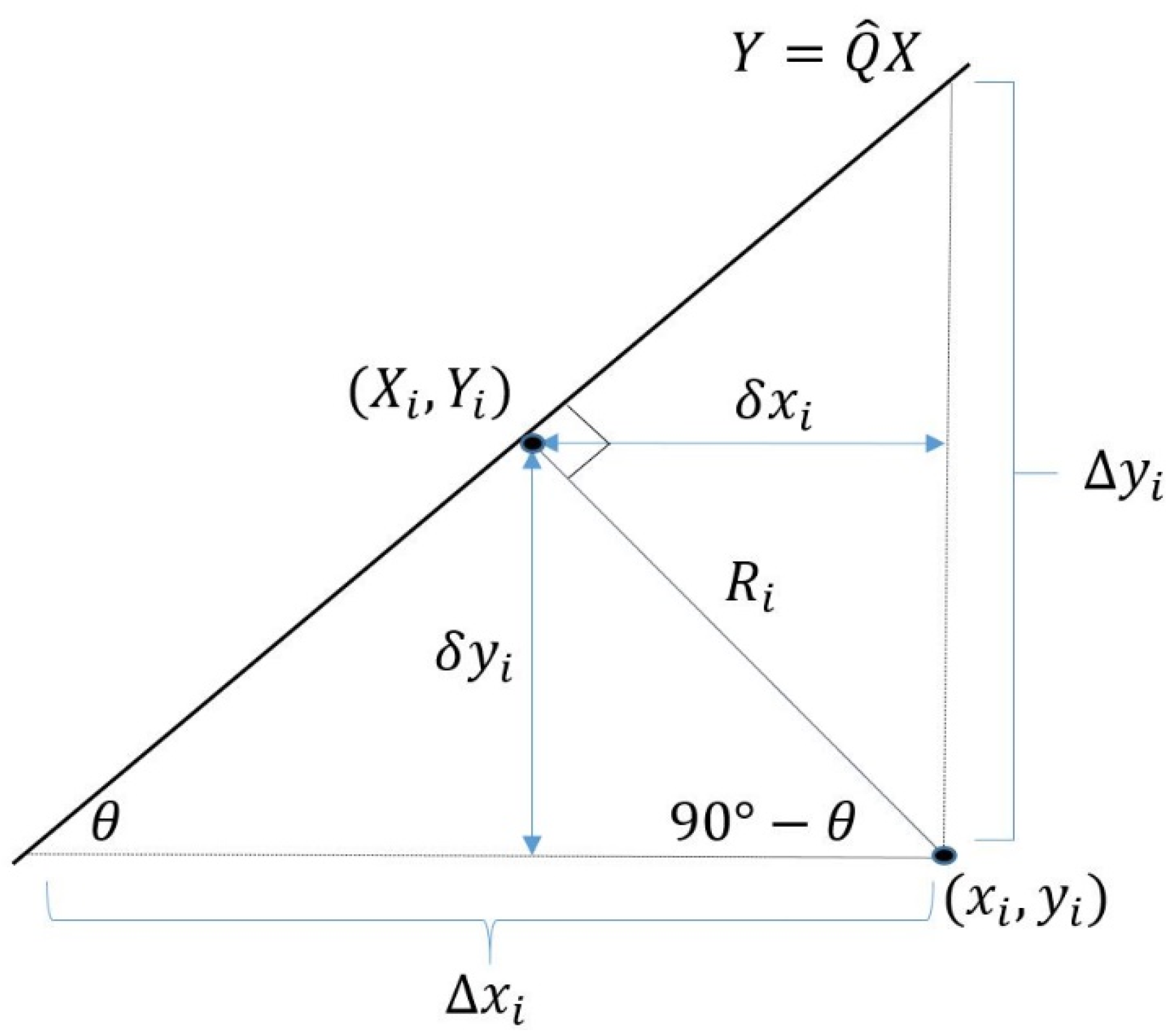
3.2.5. Geometry Method

The next proposed method is feasible to perform, but in practice, the noise of ${\sigma }_{x_i}$ and ${\sigma }_{y_i}$ are not necessarily proportional. An approach is suggested in which noise of ${\sigma }_{x_i}$ and ${\sigma }_{y_i}$ can adopt any free independent value, reaching a recursive close form solution based on geometry relationships. The geometry method is illustrated in Figure 3.

In Figure 3 there is a pair of data, $\left(x_i,y_i\right)$, which are measured $x$ and $y$, and $\left(X_i,Y_i\right)$ is the optimized image of that pair on $Y=\widehat{Q}X$. The arrows of $\delta x_i$ and $\delta y_i$ indicate uncertainties for each dimension and are proportional to ${\sigma }_{x_i}$ and ${\sigma }_{y_i}$. The variances of ${\sigma }_{x_i}^2$ and ${\sigma }_{y_i}^2$ are free as mentioned above. Therefore, the distance of $\left(x_i,X_i\right)$ is not necessarily the same as $\left(y_i,Y_i\right)$. More quality in the data measurement of $x_i$ (or $y_i$) leads to less space to its map $X_i$ ($Y_i$).

A particular state of this method is to consider equal errors, which means ${\sigma }_{x_i}$=${\sigma }_{y_i}$. In this form, the line connects $\left(x_i,y_i\right)$ and $\left(X_i,Y_i\right)$ is perpendicular to $Y=\widehat{Q}X$ line. As can be seen in Figure 3, the gradient (or slope) of $Y=\widehat{Q}X$ line is $\widehat{Q}=\Delta y_i/\Delta x_i$ and the angle of $\theta$ is equal to ${\tan }^{-1}\widehat{Q}$. The length of the perpendicular line between the data point and the line is $R_i=\Delta y_i\cos \theta =\Delta y_i/\sqrt{1+{\widehat{Q}}^2}$. Moreover, there are $\delta x_i=R_i\sin \theta$ and $\delta y_i=R_i\cos \theta$. A cost function is defined as:

$${\chi }_{geometryLS}^2={\displaystyle \sum }_{i=1}^N\frac{\delta x_i^2}{{\sigma }_{x_i}^2}+\frac{\delta y_i^2}{{\sigma }_{y_i}^2}$$

(49)

By considering $\sin {\theta }^2=1-\cos {\theta }^2=\frac{{\widehat{Q}}^2}{1+{\widehat{Q}}^2}$:

$$\delta x_i^2=\left(\frac{\Delta y_i{}^2}{1+{\widehat{Q}}^2}\right)\left(\frac{{\widehat{Q}}^2}{1+{\widehat{Q}}^2}\right);\delta y_i^2=\left(\frac{\Delta y_i{}^2}{1+{\widehat{Q}}^2}\right)\left(\frac{1}{1+{\widehat{Q}}^2}\right)$$

(50)

Moreover, by considering $\Delta y_i=y_i-\widehat{Q}{x}_i$, the cost function will be rewritten as:

$${\chi }_{geometryLS}^2={\displaystyle \sum }_{i=1}^N\frac{{\left(y_i-\widehat{Q}{x}_i\right)}^2}{{\left(1+{\widehat{Q}}^2\right)}^2}\left(\frac{{\widehat{Q}}^2}{{\sigma }_{x_i}^2}+\frac{1}{{\sigma }_{y_i}^2}\right)$$

(51)

By applying the assumption of ${\sigma }_{x_i}={\sigma }_{y_i}$ the following equation is reached:

$${\chi }_{geometryLS}^2={\displaystyle \sum }_{i=1}^N\frac{{\left(y_i-\widehat{Q}{x}_i\right)}^2}{\left(1+{\widehat{Q}}^2\right){\sigma }_i^2}$$

(52)

The above equation is equal to the Equation number (38). By adding $\gamma$ as a fading memory element to the cost function, the following equation can be achieved:

$${\chi }_{geometry-FMLS}^2={\displaystyle \sum }_{i=1}^N{\gamma }^{N-i}\frac{{\left(y_i-\widehat{Q}{x}_i\right)}^2}{\left(1+{\widehat{Q}}^2\right){\sigma }_i^2}$$

(53)

As in the previous sections, the derivative of the cost function with respect to $\widehat{Q}$ must be calculated and be set to zero in order to find the optimal value for $\widehat{Q}$.

$$\begin{array}{c}\frac{(\partial x_{(geometry-FMLS)}^2)}{\partial \stackrel{⌢}{Q}}=\frac{2}{{({\stackrel{⌢}{Q}}^2+1)}^3}{\displaystyle \sum _{i=1}^N{\gamma }^{N-i}\left[{\stackrel{⌢}{Q}}^4\left(\frac{x_i{y}_i}{{\sigma }_{x_i}^2}\right)+{\stackrel{⌢}{Q}}^3\left(\frac{2x_i^2}{{\sigma }_{x_i}^2}-\frac{x_i^2}{{\sigma }_{y_i}^2}-\frac{y_i^2}{{\sigma }_{x_i}^2}\right)+{\stackrel{⌢}{Q}}^2\left(\frac{3x_i{y}_i}{{\sigma }_{y_i}^2}-\frac{3x_i{y}_i}{{\sigma }_{x_i}^2}\right)+\stackrel{⌢}{Q}\left(\frac{x_i{}^2-2y_i{}^2}{{\sigma }_{y_i}^2}+\frac{y_i^2}{{\sigma }_{x_i}^2}\right)+\left(\frac{-x_i{y}_i}{{\sigma }_{y_i}^2}\right)\right]}\\ \end{array}$$

(54)

This equation can be rewritten in the form of:

$$\frac{\partial {\chi }_{geometry-FMLS}^2}{\partial \widehat{Q}}=\frac{2}{{\left({\widehat{Q}}^2+1\right)}^3}\left({\tilde{C}}_5{\widehat{Q}}^4+\left(-{\tilde{C}}_1+2{\tilde{C}}_4-{\tilde{C}}_6\right){\widehat{Q}}^3+\left(3{\tilde{C}}_2-3{\tilde{C}}_5\right){\widehat{Q}}^2+\left({\tilde{C}}_1-2{\tilde{C}}_3+{\tilde{C}}_6\right)\widehat{Q}-{\tilde{C}}_2\right)$$

(55)

In which ${\tilde{C}}_{1,n}=\gamma {\tilde{C}}_{1,n-1}+x_n^2/{\sigma }_{y_n}^2$; ${\tilde{C}}_{2,n}=\gamma {\tilde{C}}_{2,n-1}+x_n{y}_n/{\sigma }_{y_n}^2$; ${\tilde{C}}_{3,n}=\gamma {\tilde{C}}_{3,n-1}+y_n^2/{\sigma }_{y_n}^2$; ${\tilde{C}}_{4,n}=\gamma {\tilde{C}}_{4,n-1}+x_n^2/{\sigma }_{x_n}^2$; ${\tilde{C}}_{5,n}=\gamma {\tilde{C}}_{5,n-1}+x_n{y}_n/{\sigma }_{x_n}^2$; ${\tilde{C}}_{6,n}=\gamma {\tilde{C}}_{6,n-1}+y_n^2/{\sigma }_{x_n}^2$.

$\widehat{Q}$ is being calculated by finding the following equation roots:

$${\tilde{C}}_5{\widehat{Q}}^4+\left(2{\tilde{C}}_4-{\tilde{C}}_1-{\tilde{C}}_6\right){\widehat{Q}}^3+\left(3{\tilde{C}}_2-3{\tilde{C}}_5\right){\widehat{Q}}^2+\left({\tilde{C}}_1-2{\tilde{C}}_3+{\tilde{C}}_6\right)\widehat{Q}-{\tilde{C}}_2=0$$

(56)

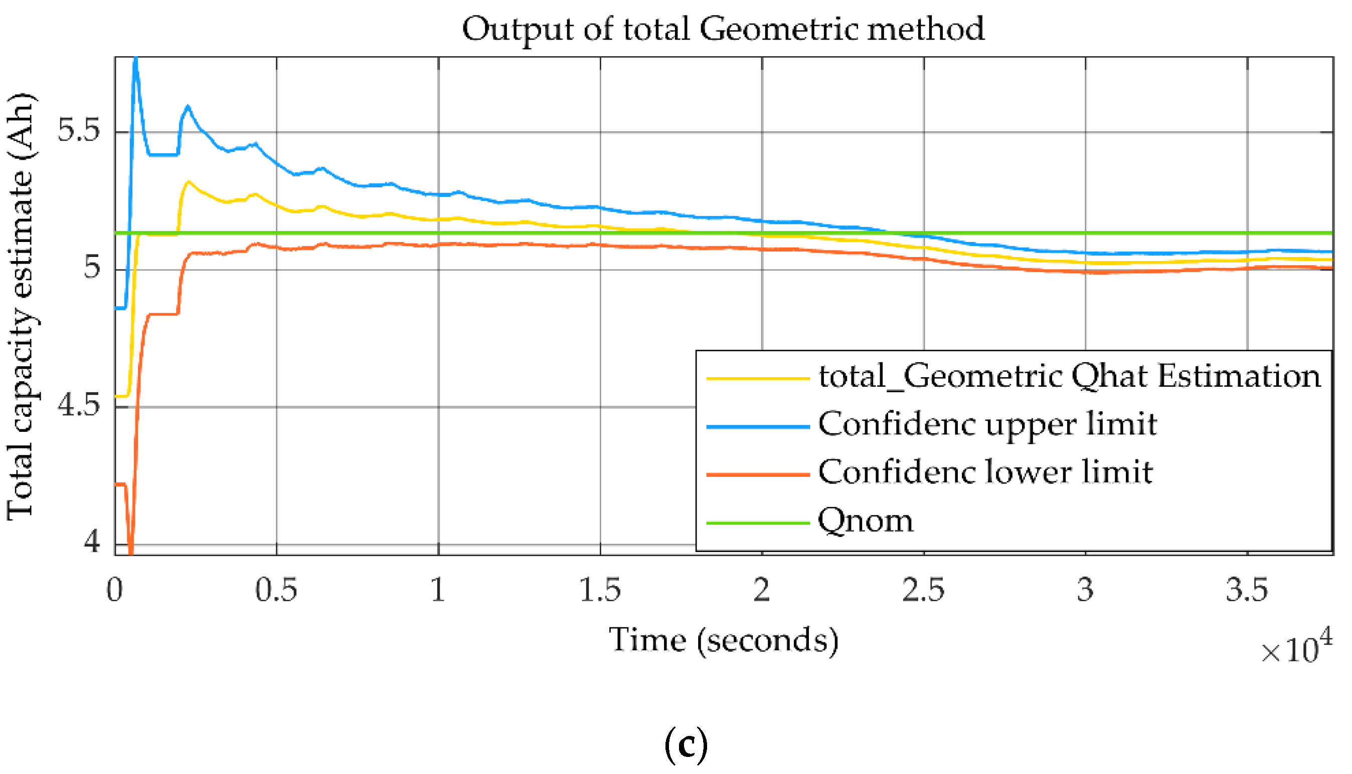
3.2.6. Total Geometry Method

As the last method the total geometry method is proposed, which can be considered as a general form of the geometry method by assuming equality in ${\sigma }_{x_i}$ and ${\sigma }_{y_i}$ values. Nevertheless, there should be a solution while these two values are not equal. When ${\sigma }_{x_i}=k{\sigma }_{y_i}$ (with variable k in different pairs of data) $y_i$ axis could be scaled as ${\tilde{y}}_i=k{y}_i$ to use the mentioned trigonometric relations of this method. Therefore, we have ${\tilde{\sigma }}_{y_i}={\sigma }_{x_i}$ and the estimated value of capacity by the scaled data is ${\widehat{Q}}_c=\widehat{Q}/k$, and clearly $k$ is estimated as $k={\sigma }_{x_i}/{\sigma }_{y_i}$.

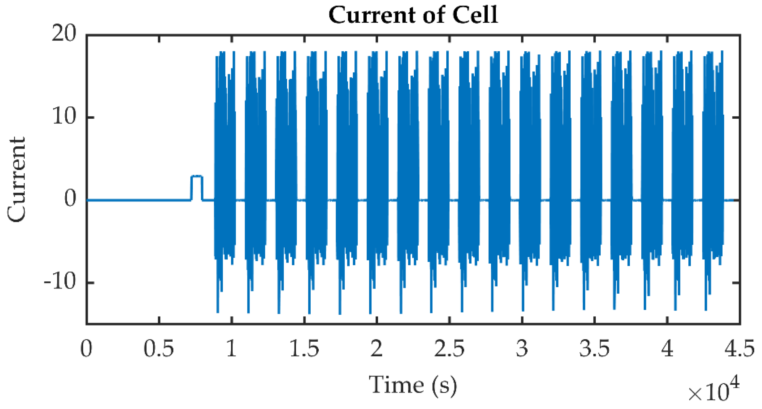
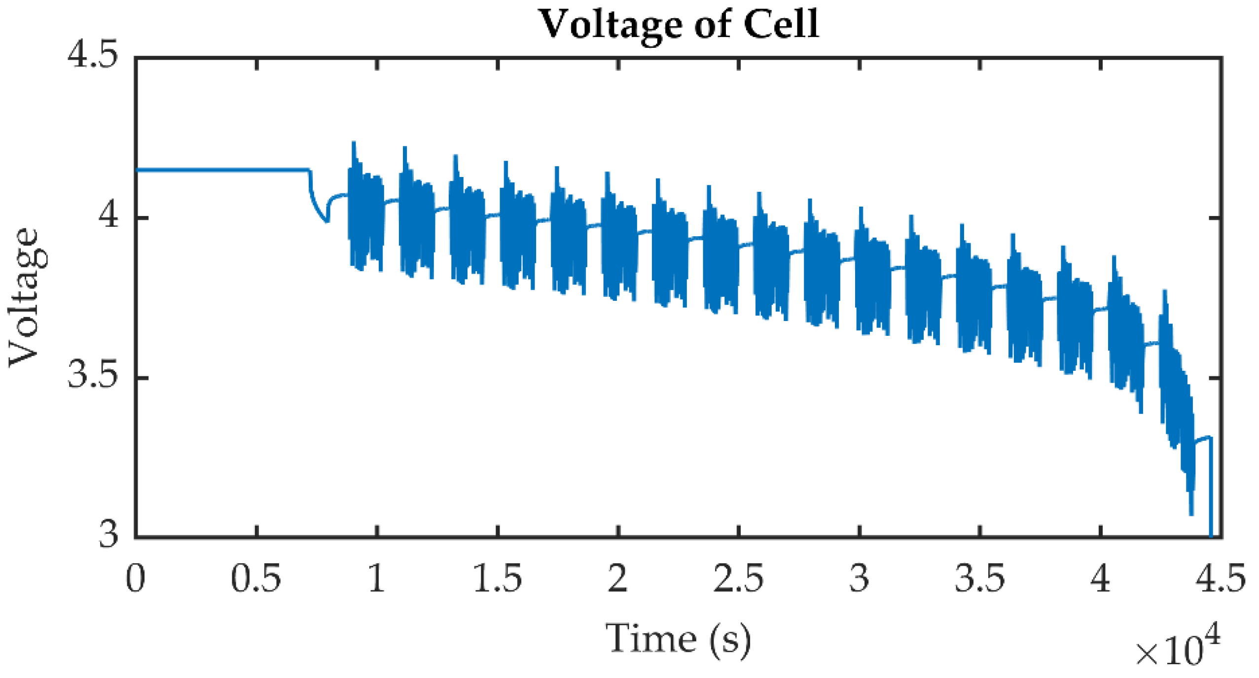
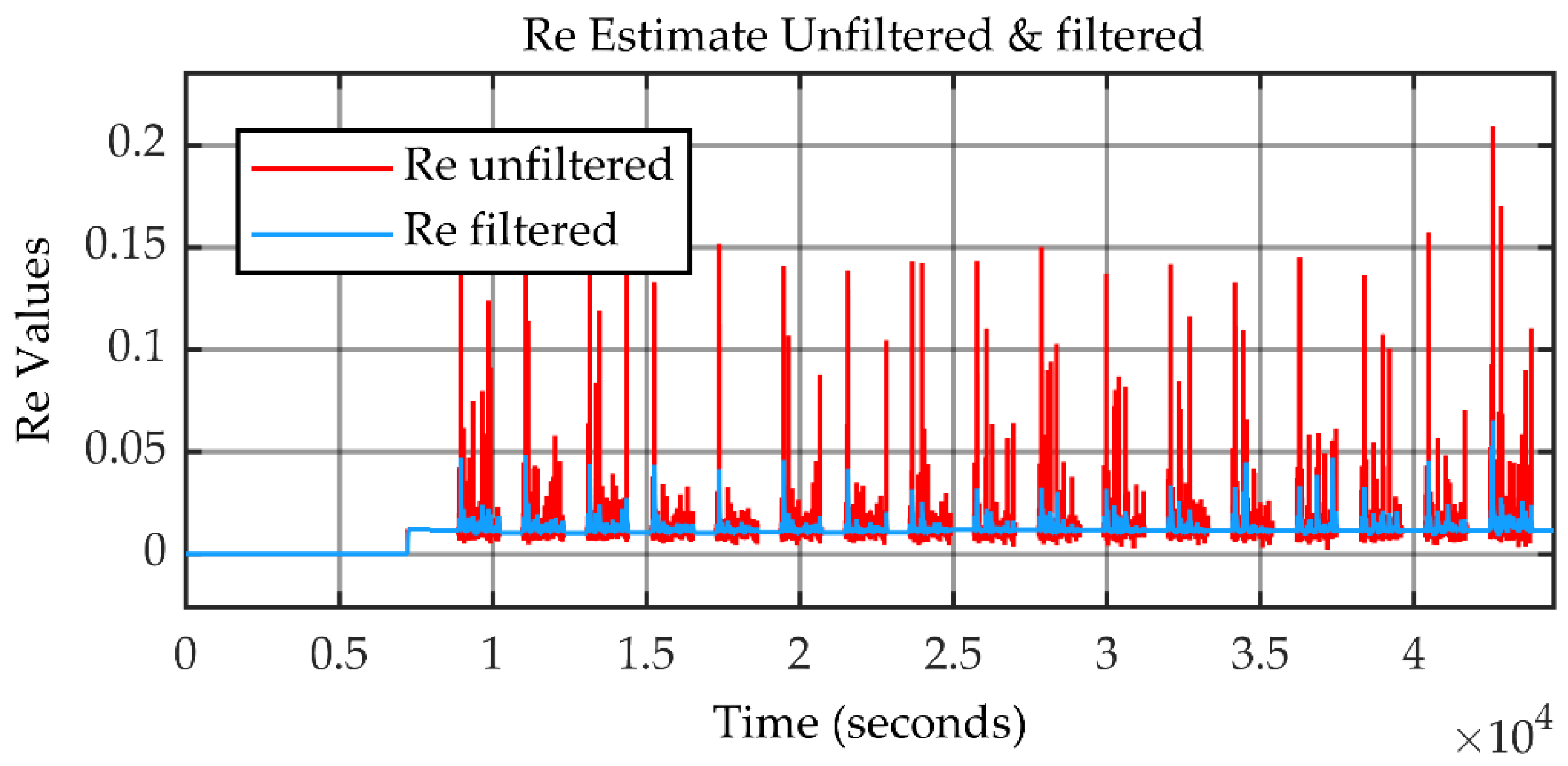
4. Validation by Experimental Data

In order to evaluate the proposed Re and capacity estimation methods, experimental data of laboratory tests at 25 °C from [29] were utilized; afterwards, a third type of least-squares method, including geometry method and total geometry method, were simulated in MATLAB. It should be noted that other types of least squares were not simulated due to not being applicable in the BMS unit. The state of charge has been estimated by the method introduced in [30]. The parameters are quantified in

Table 1. Parameter quantification.

Description of Parameter	Name of Parameter	Selected Value
Variance of x data	${\sigma }_x$	$0.01\le \mathrm{randomvalue}\le 0.02$
Variance of y data	${\sigma }_y$	$0.01\le \mathrm{randomvalue}\le 0.02$
Coefficient of filtering ${\widehat{R}}_e$	$\alpha$	0.99
Threshold of minimum current $\Delta i_b$	threshold	2
Coefficient for fading memory	$\gamma$	0.99
Coefficient of columbic efficiency	$\eta$	0.9929 (from lab data)
Nominal value of battery capacity	$Q_{nom}$	5.1314 (from lab data)

. The diagram for Re estimation is shown in Figure 4.

Experimental data of laboratory tests from [29] were utilized. Figure 5 and Figure 6 demonstrate the current and voltage characteristic of the battery, correspondingly. As can be seen, a specific load pattern was applied to the batteries. Unfiltered and filtered Re results are shown in Figure 7. The diagram of the simulation process for capacity estimation is given in Figure 8. The simulation results and the comparison of the different techniques are illustrated in Figure 9 and Figure 10, respectively. The blue and red lines represent the confidence interval of the estimated value. As observable in these diagrams, the simulation results of all methods are very close together. The total geometry method shows an initial rise, but it converges to the nominal value as with other methods in the continuation. The geometry method has all the advantages of a recursive manner, a fading memory, a close form of solution, and is considering both errors of ${\sigma }_{x_i}$ and ${\sigma }_{y_i}$. Therefore, it is applicable in embedded systems and is the most practical method.

The RMSPE (root mean square percentage error) and the MAPE (mean absolute percentage error) of the proposed methods were calculated by discharge cycle data of a roughly 9 h-long experiment, and are shown in

Table 2. Error Calculation.

Method	RMSPE	MAPE
LS3	≤0.02	≤0.015
Geometry	≤0.02	≤0.015
Total geometry	≤0.02	≤0.015

. The value of the results is based on random noise produced in MATLAB. These varied in each simulation time but were always less than 0.02%, which is a favorable method accuracy.

5. Conclusions

Lithium-ion batteries are widely used in electric vehicles due to their advantages, such as higher capacity and long cycle life, in comparison with other batteries. In this article, the lithium-ion battery capacity estimation was investigated. Analysis of state of health and remaining useful life is essential for the battery management system unit to better manage the cells in the battery pack and for better power estimation. For this purpose, a practical and confident method was proposed to estimate two essential parameters, $R_e$ and $Q$, which together represent battery state of health.

The battery’s current and voltage are the only data needed to estimate both $R_e$ and $Q$ parameters. Different approaches to the least-squares method were analyzed, and finally, the least-squares-based-geometry method was chosen. It was concluded that the least-squares techniques have many advantages. Some of the benefits of least squares methods in comparison with other methods are as follows:

• This method can estimate state of health of the battery in an online condition while the battery is being used in the vehicle (it is not only a method for the laboratory);
• It does not need extensive experiments in the laboratory to obtain charge and discharge curves;
• It does not need a significant number of datasets and learning processes;
• Even if it is better to have a more accurate model of the battery, this method can provide satisfying results without precise knowledge of the model;
• It does not have a high computational load and does not need a large data memory.

In addition, the advantage of the geometry method in comparison with other approaches of least squares is that noise of both $x_i$ and $y_i$ are considered, and it has fading memory recursive close form solution. Therefore, it is applicable in embedded systems.

The validation of the proposed methods was accomplished by using experimental data from a laboratory test of a battery. The proposed methods were applied to these data using MATLAB Simulink, the results were compared, and the errors evaluated.

References

1. Madani, S.S.; Swierczynski, M.J.; Kaer, S.K. A review of thermal management and safety for lithium ion batteries. In Proceedings of the 2017 Twelfth International Conference on Ecological Vehicles and Renewable Energies (EVER), Monte Carlo, Monaco, 11–13 April 2017; pp. 1–20. [Google Scholar]
2. Huang, R.-J.; Zhang, Y.; Bozzetti, C.; Ho, K.-F.; Cao, J.-J.; Han, Y.; Daellenbach, K.R.; Slowik, J.G.; Platt, S.M.; Canonaco, F.; et al. High secondary aerosol contribution to particulate pollution during haze events in China. Nature 2014, 514, 218–222. [Google Scholar] [CrossRef] [PubMed] [Green Version]
3. Capasso, C.; Veneri, O. Experimental analysis on the performance of lithium based batteries for road full electric and hybrid vehicles. Appl. Energy 2014, 136, 921–930. [Google Scholar] [CrossRef]
4. Madani, S.S.; Schaltz, E.; Kær, S.K. A review of different electric equivalent circuit models and parameter identification methods of lithium-ion batteries. ECS Trans. 2018, 87, 23–37. [Google Scholar] [CrossRef]
5. Dunn, B.; Kamath, H.; Tarascon, J.-M. Tarascon, electrical energy storage for the grid: A battery of choices. Science 2011, 334, 928–935. [Google Scholar] [CrossRef] [Green Version]
6. Chen, W.; Liang, J.; Yang, Z.; Li, G. A review of lithium-ion battery for electric vehicle applications and beyond. Energy Procedia 2019, 158, 4363–4368. [Google Scholar] [CrossRef]
7. Hu, Y.; Yurkovich, S.; Guezennec, Y.; Yurkovich, B. Electro-thermal battery model identification for automotive applications. J. Power Sources 2011, 196, 449–457. [Google Scholar] [CrossRef]
8. Li, Y.; Zou, C.; Berecibar, M.; Nanini-Maury, E.; Chan, J.C.-W.; Bossche, P.V.D.; Van Mierlo, J.; Omar, N. Random forest regression for online capacity estimation of lithium-ion batteries. Appl. Energy 2018, 232, 197–210. [Google Scholar] [CrossRef]
9. El Mejdoubi, A.; Oukaour, A.; Chaoui, H.; Gualous, H.; Sabor, J.; Slamani, Y. State-of-charge and state-of-health lithium-ion batteries’ diagnosis according to surface temperature variation. IEEE Trans. Ind. Electron. 2015, 63, 2391–2402. [Google Scholar] [CrossRef]
10. Ungurean, L.; Cârstoiu, G.; Micea, M.V.; Groza, V. Battery state of health estimation: A structured review of models, methods and commercial devices. Int. J. Energy Res. 2017, 41, 151–181. [Google Scholar] [CrossRef]
11. She, C.; Li, Y.; Zou, C.; Wik, T.; Wang, Z.; Sun, F. Offline and online blended machine learning for lithium-ion battery health state estimation. IEEE Trans. Transp. Electrif. 2021. [Google Scholar] [CrossRef]
12. Krupp, A.; Ferg, E.; Schuldt, F.; Derendorf, K.; Agert, C. Incremental capacity analysis as a state of health estimation method for lithium-ion battery modules with series-connected cells. Batteries 2021, 7, 2. [Google Scholar] [CrossRef]
13. Zhang, S.; Guo, X.; Dou, X.; Zhang, X. A rapid online calculation method for state of health of lithium-ion battery based on coulomb counting method and differential voltage analysis. J. Power Source 2020, 479, 228740. [Google Scholar] [CrossRef]
14. Chen, Z.; Mi, C.C.; Fu, Y.; Xu, J.; Gong, X. Online battery state of health estimation based on Genetic Algorithm for electric and hybrid vehicle applications. J. Power Sources 2013, 240, 184–192. [Google Scholar] [CrossRef]
15. Landi, M.; Gross, G. Measurement techniques for online battery state of health estimation in vehicle-to-grid applications. IEEE Trans. Instrum. Meas. 2014, 63, 1224–1234. [Google Scholar] [CrossRef]
16. Hannan, M.A.; Lipu, M.S.H.; Hussain, A.; Saad, M.H.; Ayob, A. Neural network approach for estimating state of charge of lithium-ion battery using backtracking search algorithm. IEEE Access 2018, 6, 10069–10079. [Google Scholar] [CrossRef]
17. Watrin, N.; Blunier, B.; Miraoui, A. Review of adaptive systems for lithium batteries state-of-charge and state-of-health estimation. In Proceedings of the 2012 IEEE Transportation Electrification Conference and Expo (ITEC), Dearborn, MI, USA, 18–20 June 2012; pp. 1–6. [Google Scholar]
18. Hu, X.; Li, S.; Jia, Z.; Egardt, B. Enhanced sample entropy-based health management of Li-ion battery for electrified vehicles. Energy 2014, 64, 953–960. [Google Scholar] [CrossRef]
19. Kelsey, B.; Hatzell, A.S.; Hosam, K.F. A survey of long-term health modeling, estimation, and control of Lithium-ion batteries: Challenges and opportunities. In Proceedings of the 2012 American Control Conference (ACC), Montreal, QC, Canada, 27–29 June 2012. [Google Scholar]
20. Kim, J.; Shin, J.; Chun, C.; Cho, B.H. Stable configuration of a li-ion series battery pack based on a screening process for improved voltage/SOC balancing. IEEE Trans. Power Electron. 2012, 27, 411–424. [Google Scholar] [CrossRef]
21. Burgos-Mellado, C.; Orchard, M.E.; Kazerani, M.; Cárdenas, R.; Sáez, D. Particle-filtering-based estimation of maximum available power state in Lithium-Ion batteries. Appl. Energy 2016, 161, 349–363. [Google Scholar] [CrossRef]
22. Vetter, J.; Novák, P.; Wagner, M.R.; Veit, C.; Möller, K.-C.; Besenhard, J.O.; Winter, M.; Wohlfahrt-Mehrens, M.; Vogler, C.; Hammouche, A. Ageing mechanisms in lithium-ion batteries. J. Power Source 2005, 147, 269–281. [Google Scholar] [CrossRef]
23. Groot, J. State-of-Health Estimation of Li-Ion Batteries: Cycle Life Test Methods; Chalmers Tekniska Hogskola: Gothenburg, Sweden, 2012. [Google Scholar]
24. Madani, S.S.; Schaltz, E.; Kær, S.K. An electrical equivalent circuit model of a lithium titanate oxide battery. Batteries 2019, 5, 31. [Google Scholar] [CrossRef] [Green Version]
25. Sun, T.; Jiang, S.; Li, X.; Cui, Y.; Lai, X.; Wang, X.; Ma, Y.; Zheng, Y. A novel capacity estimation approach for lithium-ion batteries combining three-parameter capacity fade model with constant current charging curves. IEEE Trans. Energy Convers. 2021, 36, 2574–2584. [Google Scholar] [CrossRef]
26. Choi, Y.; Ryu, S.; Park, K.; Kim, H. Machine learning-based lithium-ion battery capacity estimation exploiting multi-channel charging profiles. IEEE Access 2019, 7, 75143–75152. [Google Scholar] [CrossRef]
27. Li, W.; Sengupta, N.; Dechent, P.; Howey, D.; Annaswamy, A.; Sauer, D.U. Online capacity estimation of lithium-ion batteries with deep long short-term memory networks. J. Power Source 2021, 482, 228863. [Google Scholar] [CrossRef]
28. He, Y.; He, R.; Guo, B.; Zhang, Z.; Yang, S.; Liu, X.; Zhao, X.; Pan, Y.; Yan, X.; Li, S. Modeling of Dynamic Hysteresis Characters for the Lithium-Ion Battery. J. Electrochem. Soc. 2020, 167, 090532. [Google Scholar] [CrossRef]
29. University of Maryland Website. Available online: https://calce.umd.edu/battery-data (accessed on 1 October 2021).
30. Al-Gabalawy, M.; Hosny, N.S.; Dawson, J.A.; Omar, A.I. State of charge estimation of a Li-ion battery based on extended Kalman filtering and sensor bias. Int. J. Energy Res. 2020, 45, 6708–6726. [Google Scholar] [CrossRef]
Figure 1. Loss in battery total capacity versus time: (a) normal transition of ions between electrodes. (b) Effect of side reaction on transition. (c) Impact of structural decay on ion loss.
Batteries 08 00031 g001
Figure 2. Equivalent circuit model.
Batteries 08 00031 g002
Figure 3. Geometry method.
Batteries 08 00031 g003
Figure 4. Re estimation diagram.
Batteries 08 00031 g004
Figure 5. Battery current characteristic.
Batteries 08 00031 g005
Figure 6. Battery voltage characteristic.
Batteries 08 00031 g006
Figure 7. Unfiltered and filtered Re.
Batteries 08 00031 g007
Figure 8. Total Q estimation diagram.
Batteries 08 00031 g008
Figure 9. The results of simulation for (a) least squares method, (b) geometry method, (c) total geometry method.
Batteries 08 00031 g009aBatteries 08 00031 g009b
Figure 10. Comparison of different methods.
Batteries 08 00031 g010