1. Introduction
Fatal traffic accidents are a major and widespread problem in the United States and worldwide. In the U.S. alone, thousands of individuals lose their lives each year due to these incidents, while road accidents are considered the ninth leading cause of death worldwide. According to the World Health Organization, approximately 1.3 million deaths occur annually from road accidents, causing around 50 million injuries across different countries [
1]. However, initiatives such as the United Nations Global Plan aim to reduce road fatalities and injuries by half by 2030, giving optimism for improvement. [
2].
To effectively prevent fatal accidents, it is crucial to develop strategies grounded in a thorough understanding of the various contributing factors. These encompass a range of elements from human behavior and vehicle malfunctions to environmental conditions and broader macrosocioeconomic influences [
3]. Recent extensive research has demonstrated a mutual coordination between road transportation and economics [
4], highlighting how economic status can influence regional disparities in crash occurrences [
5]. This underscores the importance of considering a diverse array of factors in devising comprehensive accident prevention strategies.
Understanding the impact of socioeconomic factors on fatal collisions requires a clear definition and comprehension of these factors themselves. These factors include broader social, economic, and demographic conditions such as Gross Domestic Product (GDP), inflation rate, income levels, educational attainment, poverty rates, employment rates, average cost per mile traveled, daily vehicle miles traveled by drivers, and the extent of urban development in a particular area. Researchers have extensively studied these factors [
5,
6,
7]. Previous studies have typically focused on individual contributing factors or a limited combination. However, it is crucial to analyze the combined influence of various macrosocioeconomic factors on the occurrence of deadly accidents.
This research aims to unravel the combined impact of socioeconomic, demographic, and technological factors that, through a complex interplay, contribute to the overall number of traffic-related fatalities. In addition to examining individual factors, this study seeks to shed light on the intricate relationships between these variables and how they can affect the total number of deaths resulting from traffic incidents. It is crucial to understand that this research is exploratory in nature, rather than confirmatory. This means that the primary objective is not to establish causal relationships, but rather to observe patterns and correlations that have already been identified and substantiated in the field. It is important to note that this approach is useful for generating hypotheses and identifying potential areas for further research. In addition, the investigation of such a complex structure could be based on a myriad of other influencing factors. In this study, our focus is on a country like the United States, which presents a unique context with its specific socioeconomic dynamics, demographic diversity, and technological advances. By concentrating on this particular setting, we aim to provide insights that are relevant and adaptable to similar contexts, while acknowledging that findings may vary in different national or regional scenarios.
After conducting a thorough review of the existing literature, this study identifies three primary categories of factors that contribute to fatal accident rates: demographic, socioeconomic, and technological. In the following sections, each of these categories will be discussed in detail, drawing from relevant research and integrating the findings into a cohesive analytical framework.
This article is structured in a methodical manner with subsequent sections to ensure clarity and continuity.
Section 2 will explain the methodologies used to acquire and prepare the datasets for this study. Following that,
Section 3 will describe the analytical approach adopted, specifically the Lasso polynomial regression model, and how it will be applied to the data. Finally,
Section 4 will present the findings of the model, highlighting new insights and contributing to the ongoing discussion within the research community on traffic safety and its underlying factors. Through this structured discourse, this study aims to improve the understanding of traffic fatalities and provide a foundation for future research in this critical domain.
1.1. Impact of Demographic Factors
In the collection of factors that contribute to traffic safety, demographic characteristics provide the foundational context to understand patterns and trends in road use and its associated risks. Average family size, higher educational attainment, and population collectively paint a picture of the social makeup that is intrinsic to the way individuals interact with transportation systems. Demographic elements such as average family size, higher educational attainment, and population serve as the underlying strata upon which socioeconomic influences and technological advancements exert their effects, making them indispensable for a holistic analysis of traffic fatality risks.
High population density and urbanization levels generally lead to more traffic fatalities due to increased traffic density and complex road networks and age distribution within the population [
8,
9]. The age distribution of drivers is important for road safety, as both younger and older drivers pose specific risks. [
10].
Research shows that young drivers possess an exaggerated sense of their driving ability, which apparently leads to a lower appreciation of the level of danger associated with different driving actions and therefore to greater risk-taking behaviors while driving [
11,
12]. Larger family sizes may influence vehicle occupancy and travel frequency, while higher levels of educational attainment often correlate with greater awareness of safety protocols and potentially influence commute patterns [
13,
14].
1.2. Impact of Socioeconomic Factors
Socioeconomic factors refer to the social and economic aspects of a community or society, which are often related to economic activity and policy. It is important to note that while some factors are clearly socioeconomic or demographic in nature, others can potentially intersect both categories. For example, higher educational attainment can have socioeconomic implications, influencing income levels and employment opportunities. Therefore, the classification provided here is based on the primary association of each factor.
Socioeconomic factors play a crucial role in shaping transportation behaviors and influencing the risk of traffic-related fatalities. These factors include a wide range of economic activities, policies, and societal behaviors. For example, the number of registered cars in a society is indicative of its mobility needs and economic capabilities. The number of registered vehicles has increased over time, but the impact on the number of accidents is not clear. Some studies suggest that accidents cannot influence vehicle registration, while others indicate that accidents can cause changes in vehicle registration [
15].
The GDP is a measure of the economic health of a community. GDP per capita is a crucial indicator of a country’s economic output and living standards. Research suggests that an increase in GDP per capita is associated with a decrease in traffic accidents due to better infrastructure, improved road safety measures, and increased awareness of and education on traffic regulations [
16,
17,
18]. Furthermore, the inflation rate has a significant impact on the occurrence of fatal crashes; higher inflation rates may result in higher vehicle maintenance costs, leading to delayed or inadequate vehicle upkeep [
19,
20].
The economic stability of individuals is directly affected by the annual average unemployment rate, the average household income, and the minimum wage. This, in turn, affects their travel habits and vehicle maintenance practices. The role of the minimum wage in traffic safety is complex, but critical. Lower minimum wages are often associated with higher poverty rates and income inequality, which, in turn, correlate with inadequate vehicle maintenance and limited access to safer transportation options. However, this relationship is not linear. Studies show that an increase of
in the minimum wage could correspond to an increase of
to
in traffic accidents [
21]. Various studies suggest that higher income and education levels are associated with a lower probability of deadly accidents [
22,
23] and that poverty rates are positively correlated with the occurrence of fatal accidents [
24].
Investing in transportation and infrastructure development is crucial to ensure the safety and efficiency of road networks. Countries that allocate a larger portion of their budget to these sectors generally report fewer traffic fatalities [
25]. However, it is important to note that the immediate impact of such investments may not always result in lower fatal traffic. As infrastructure and transportation systems improve, increased construction and maintenance activities may temporarily contribute to increased traffic volumes and potential hazards [
26,
27].
VMT, average total cost per mile, and average annual fuel price are used as indicators of the economic burden of transportation and the broader economic patterns that influence individual behavior. Although VMT has a clear impact on motor vehicle fatalities, it is difficult to isolate and quantify its individual effects due to the interplay between driving demand and other factors, such as fuel price or average cost per mile. Studies have shown that fuel prices are significantly correlated with the rate of fatal accidents [
28]. When fuel prices rise, there is often a corresponding decrease in fatal accidents, likely due to reduced travel demand, shorter travel distances, and more efficient route planning [
29,
30].
Alcohol consumption is often used as a measure of social behavior and economic spending patterns. It is influenced by various factors, such as disposable income, cultural practices, social norms, and stress levels, all of which are related to socioeconomic conditions. Driving under the influence of alcohol and/or psychoactive substances increases the risk of serious and even fatal motor vehicle accidents [
31,
32]. In addition, the interaction of average alcohol consumption with other socioeconomic factors adds a layer of complexity to its impact on traffic safety. Economic downturns, characterized by factors such as reduced household income and austerity measures, could alter drinking behaviors, limiting opportunities for consumption or, conversely, increasing it due to stress and social disruption.
The laws and regulations imposed by the party in power can have a direct influence on many of the socioeconomic factors discussed in this document. We would like to further explore whether a shift in political party has a substantial effect on the total number of fatal accidents, and thus, we include this as one of the variables in our research.
The interplay of various socioeconomic factors creates a complicated network that influences how people use vehicles, affects road safety, and ultimately determines the number of fatal traffic accidents each year. It is crucial to study these factors to develop well-informed policies that address the economic causes of transportation safety issues.
1.3. Impact of Technological and Safety Features
The evolution of technology within the automotive industry has led to the implementation of various safety features and technologies aimed at reducing the number of fatal traffic accidents. These enhancements, encompassing a wide array of features, technologies, and design principles, are primarily focused on augmenting the safety of drivers and passengers. The primary objective of these innovations is to decrease the likelihood of accidents, mitigate the severity of crash injuries, and enhance road safety.
Advanced Driver Assist Systems are central to these technological advancements, including adaptive cruise control, lane-keeping assistance, blind spot monitoring, and automatic emergency braking. These systems are classified into different levels of automation, from partial to conditional automation. Research indicates that the utilization of ADAS can reduce traffic fatalities by diminishing human error [
33]. It is suggested that fully autonomous driving systems are necessary to completely eliminate fatal road accidents in the future [
34]; another critical safety feature is electronic stability control, which helps drivers maintain vehicle control in difficult driving conditions [
35].
Most road accidents arise from human error. Advanced driver assistance systems are developed to enhance vehicle safety by automating and adapting vehicle systems. These automated features have been shown to reduce traffic fatalities by minimizing human errors. ADAS technology has gained significant attention as a research topic over the past decade, designed to provide critical information for drivers in order to decrease the number of traffic accidents. A variety of ADASs currently under investigation for intelligent vehicles are based on Artificial Intelligence, Laser, and Computer Vision technologies with the potential to decrease both the frequency and severity of traffic accidents. This leads us towards fully autonomous driving systems as essential to achieving zero fatal road traffic accidents.
To support this investigation, a report by the National Highway Traffic Safety Administration highlighted a significant decrease of
in the fatality rate per vehicle mile of travel from 1960 to 2012 [
36]. This decline has been attributed, in part, to the introduction of vehicle safety technologies such as seatbelts, airbags, and electronic stability control (ESC) in conjunction with programs aimed at promoting the usage of these safety features. This study will also consider the influence of these technological factors in the context of road safety.
2. Model Development
The impact of socioeconomic, demographic, and technological factors on the prevalence of fatal traffic accidents is a complex issue. Studies have shown that the correlation between economics and traffic fatalities follows a curved pattern similar to an inverted U [
37,
38]. At the beginning of an economic downturn, the initial decline in traffic volume due to factors such as job loss and reduced consumer spending can result in a decrease in accidents. But as the recession deepens, other factors can increase the risk of accidents, such as reduced investment in road infrastructure, decreased spending on vehicle maintenance, and potential increases in risky behaviors such as driving under the influence, possibly due to stress or other social problems related to the recession. These factors can lead to an eventual increase in fatal accidents, even with lower traffic volumes [
39]. At the onset of economic growth, there is often an increase in vehicle ownership and usage, as more people can afford cars and there is greater mobility for work and leisure. This increase in traffic volume can lead to an initial increase in accidents. However, as the economy continues to grow and stabilize, factors such as improved road safety measures, better infrastructure, greater public awareness, and the ability to afford safer vehicles come into play, leading to a reduction in the number of fatal accidents [
26,
40].
The study of the correlation between traffic accidents and socioeconomic factors is a multifaceted issue that requires careful examination. Various nonlinear modeling techniques, such as decision trees and random forests, have been used to investigate the severity of accidents and their relationship with socioeconomic factors [
41,
42,
43,
44,
45]. Furthermore, advanced machine learning models like neural networks have been widely used to explore the impact of socioeconomic factors on fatal accidents [
46,
47,
48]. These approaches have provided valuable information on the complex relationship between traffic accidents and socioeconomic factors and have the potential to inform the development of effective accident prevention strategies.
It is crucial to conduct comprehensive research on the intricate interplay of socioeconomic factors that lead to fatal accidents. Although advanced machine learning techniques such as neural networks have been adopted, comprehending and interpreting the results of these models still pose a significant challenge. Addressing these research gaps is paramount to develop effective policies, gain insight into the underlying determinants of fatal accidents, and create preventive measures. Consequently, it is critical that we prioritize efforts to bridge these gaps and continue to explore this vital area of study.
In this study, we conducted a comprehensive analysis of various factors, as outlined in
Table 1, with the aim of establishing a causal relationship between these variables and traffic fatalities. To examine the complex nonlinear dynamics at play, we employed a polynomial regression model of degree 2, utilizing a Lasso model to optimize the machine learning approach. This approach is well known for its efficacy in variable selection, regularization, and reduction in overfitting. By minimizing residual error while imposing constraints on the model parameters, we encourage sparsity and ensure optimal results [
49]. It is important to note that the utilization of this technique has provided us with an effective means of examining the multifaceted nature of the data, allowing us to draw meaningful conclusions that have significant implications for this field of study.
In order to model the relationship between the independent variables listed in
Table 1 and the number of fatal crashes, we utilize the equation
This second-degree polynomial transformation is employed to capture any nonlinear associations that may exist between the variables and the occurrence of deadly accidents. Lasso regression is then used to identify the pivotal variables and their coefficients, which in turn minimizes prediction errors. To ensure that these coefficients remain within reasonable bounds, a regularization parameter is incorporated to constrain the sum of the absolute value of the regression coefficients. This approach yields a more accurate and meaningful understanding of the factors that contribute to fatal crashes, thereby informing efforts to prevent such tragic events in the future.
3. Data
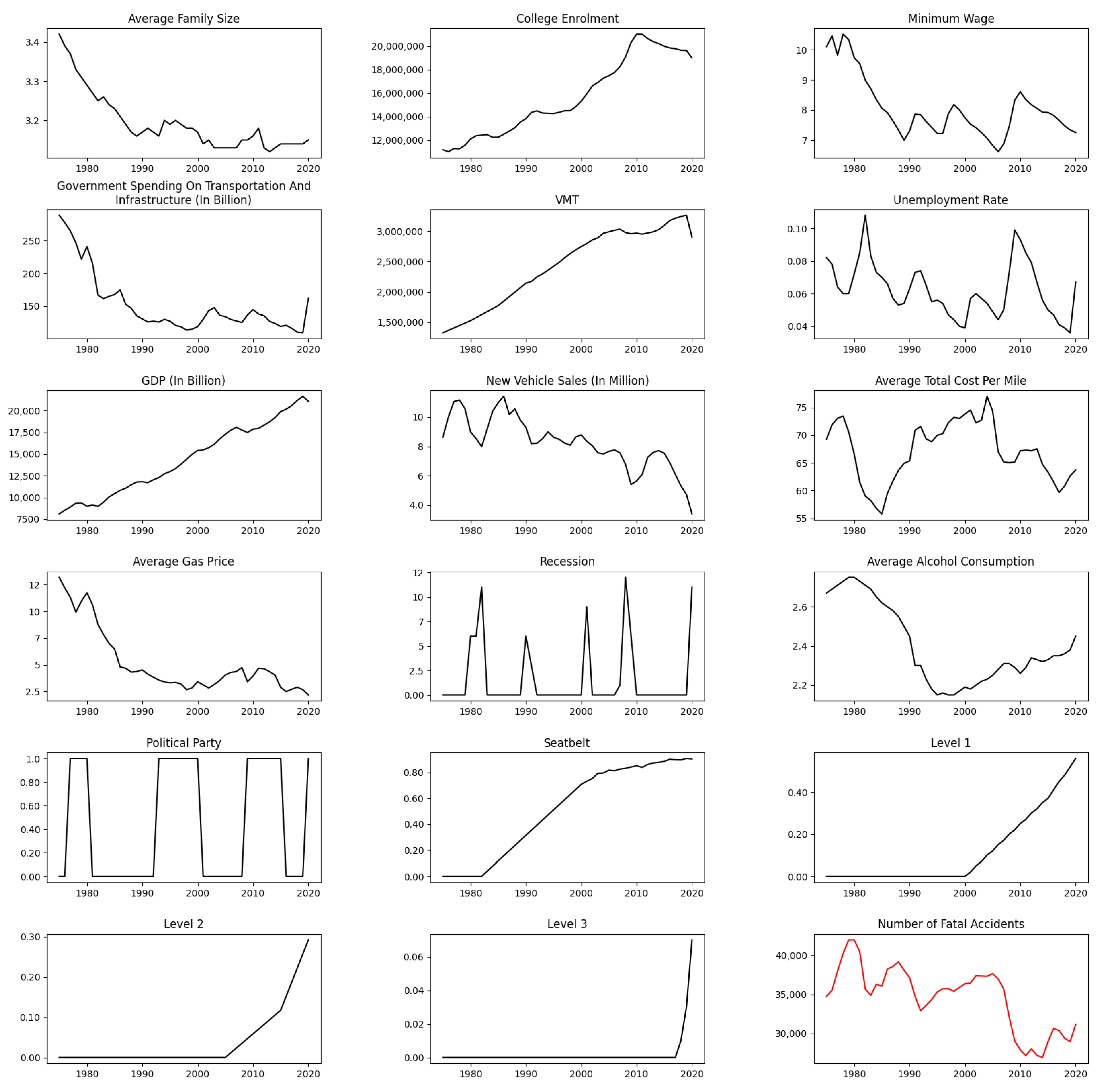
This study is based on an extensive dataset that covers the number of fatal accidents in the United States from 1975 to 2020. The data were sourced from reputable government agencies like the Federal Highway Administration, Department of Labor, and Department of Commerce, and they include a range of socioeconomic indicators. To ensure accurate analysis, all monetary values have been adjusted to their 2020 equivalent to account for the effects of inflation. Overall, the dataset provides a solid foundation for this academic research.
The visual representation shown in
Figure 1 presents a comprehensive overview of the demographic, socioeconomic and various other variables that have been taken into account in this study. It should be noted that the data do not reveal any direct linear correlation between any single variable and the number of fatal accidents.
The column labeled recession provides a detailed account of the duration of economic recessions in months. Economic recessions are defined as significant and prolonged declines in a country’s economic activity, often marked by decreased GDP and negative trends in employment, consumer spending, business investment, and industrial production.
The variable governing political party serves as an indicator of the governing political party during the specified study period. As political parties typically have diverse policies and priorities, particularly in domains such as infrastructure and transportation, they can have diverse impacts on road safety in both the short and long run. For this particular study, the Republican and Democratic parties were assigned binary codes of 0 and 1, respectively.
To further analyze the data presented in the seatbelt and autonomous feature columns, it is important to dig deeper into the academic research surrounding these topics. Numerous studies have shown that seatbelt use significantly reduces the risk of injury or death in a car accident. Additionally, research on autonomous features has shown promising results in terms of improving road safety. As these technologies continue to advance, it is essential to remain informed and educated about their potential benefits and limitations.
The dataset used in this empirical investigation was divided into two distinct segments, in which a considerable proportion of of the total data was apportioned for the purpose of model training and adjustment, while the remaining of the data was used for the evaluation of the generalizability of the model to novel data. It is worth noting that the Lasso polynomial regression model is used primarily for data mining activities and not for predictive analytics. Nonetheless, its competence and dependability remain of paramount importance, which is ensured through rigorous training and validation on both datasets. To optimize the parameters, a grid search was performed, resulting in the attainment of model training and test r2-scores of 0.98 and 0.94, respectively, with a regularization parameter . The r2-scoring function in machine learning, also known as the coefficient of determination, measures the proportion of the variance in the dependent variable that is predictable from the independent variables, providing an indication of the goodness of fit of a model.
Tibshirani [
50] suggested that the Lasso model has a significant advantage over other models due to its L1 regularization. This regularization technique promotes sparsity in feature coefficients, simplifying the model and reducing overfitting by preventing noise capture. Additionally, the Lasso model effectively addresses multicollinearity, allowing for the identification of significant individual features in highly correlated datasets. As shown in
Figure 2, the coefficients derived from the Lasso model exclude features with a coefficient of zero.
In a Lasso regression model, coefficients play a crucial role in understanding the influence of predictor variables on the response variable. Positive coefficients in a Lasso model indicate a direct relationship, meaning that as the predictor variable increases, the response variable tends to increase as well. This positive correlation suggests that the feature positively contributes to or is associated with an increase in the outcome being predicted. On the other hand, negative coefficients signify an inverse relationship. In this case, an increase in the predictor variable is associated with a decrease in the response variable. This negative correlation implies that the feature is inversely related to or diminishes the outcome. The Lasso model is particularly adept at feature selection, as it can shrink less important variable coefficients to zero, effectively removing them from the model. This helps in isolating the variables that are most predictive and simplifying the model by eliminating irrelevant features, leading to a more interpretable and less complex model.
4. Results
The coefficients derived from the Lasso regression model are a critical analytical tool to determine the importance of various predictors for the frequency of fatal traffic accidents. The model shows that certain features, such as government spending on infrastructure and transportation and average total cost per mile, have a positive linear correlation with the number of fatal accidents. This means that an increase in these variables is associated with a corresponding increase in the predicted number of fatal accidents. This conclusion is consistent with previous scholarly investigations of these factors [
25,
26,
40,
51,
52].
The results of this model indicate that there is an inverse relationship between the frequency of fatal accidents and several other variables, such as governing political party, level 3 autonomous features, ESC, five-star enhancement, and the use of a safety app. This means that improvements or increases in these features are likely to reduce the number of fatal crashes. These findings support earlier discussions and research on the impact of these factors on road safety, highlighting the complex nature of influences on traffic accident rates. This underscores the importance of a comprehensive approach in the management of traffic safety and the formulation of policies. References supporting these findings include [
33,
34,
35,
53,
54,
55,
56].
Our model discovered a nonlinear relationship between the frequency of fatal accidents and four independent variables. These variables are the average family size, the unemployment rate, the average alcohol consumption, and their squared values. The correlation is particularly strong when the nonlinearities of these variables are taken into account. One noteworthy finding is that the average alcohol consumption has a positive correlation when squared. This indicates that the number of fatal accidents increases nonlinearly in proportion to the square of the average alcohol consumption. This positive quadratic coefficient implies a U-shaped relationship, wherein the dependent variable initially increases and subsequently decreases as the independent variable ascends.
There is also an inverse relationship between the unemployment rate and average family size with the number of fatal accidents. This relationship is indicated by a negative degree-two polynomial correlation. This suggests that an increase in these variables is associated with a more significant decrease in fatal accidents. Additionally, the presence of a negative quadratic coefficient indicates an inverted U-shaped curve.
Furthermore,
Figure 2 elucidates the interactions among higher-order features, essentially delineating the interplay of the primary features. The linear coefficient for an interaction term, denoted as
, indicates the variation in the dependent variable as a result of a unit change in one of the interacting variables (
or
), while maintaining the other constant. A positive linear coefficient for
implies that an increase in the value of
exerts a beneficial influence on the dependent variable when
is constant, whereas a negative coefficient suggests an adverse effect.
In terms of quadratic coefficients for interaction terms, these coefficients elucidate the nonlinear or curvilinear dynamics between the interaction term and the dependent variable. A positive quadratic coefficient for indicates a U-shaped curve in the relationship, suggesting that as the product of and increases, the dependent variable initially rises before eventually declining. On the contrary, a negative quadratic coefficient represents an inverted U-shaped curve.
The interpretation of interaction terms with quadratic coefficients can be complicated considering the complex interaction and its nonlinear impact on the dependent variable. Thus, the use of graphical representations or contour plots is often beneficial for clarifying these relationships.
Figure 3 presents a contour plot generated from the Lasso polynomial regression analysis of the dataset. Contour plots graphically depict the relationships between two predictor variables and the response variable, utilizing the
x and
y axes for the predictor variables and contour lines or color gradations to represent the response variable’s values. This visualization facilitates an understanding of how the response variable changes across the ranges of the predictor variables.
In contour plots, the shading density is integral to data interpretation. Regions with denser shading, depicted as darker areas, typically indicate a higher concentration of data points, suggesting a more robust correlation or significant relationship between the variables at these points. Conversely, lighter shaded areas denote a smaller density of data points, which may point to a weaker or less defined relationship.
Contour plots are invaluable for visualizing both the direction and magnitude of relationships between variables. The patterns of the contour lines provide key insights; converging contour lines imply a synergistic interaction, indicating that the combined influence of the variables is greater than their individual effects. On the other hand, divergent contour lines indicate an antagonistic interaction, where the combined effect of the variables is weaker than expected. In
Figure 3, this concept is visually demonstrated: darker regions signal areas of convergence, suggesting more powerful synergistic interactions, while lighter regions point to divergence, indicating weaker antagonistic interactions. Thus, the darker regions in the plot are pivotal in identifying where the response variable reaches its optimal values, shedding light on the intricate relationships among the variables. Based on previous research, there is a negative correlation between the unemployment rate and the average family size and the number of fatal accidents [
57,
58]. This means that an increase in these variables is associated with a decrease in fatal accidents. Additionally, the presence of a negative quadratic coefficient indicates an inverted U-shaped curve.
Furthermore,
Figure 2 illustrates the interactions among higher-order features, essentially delineating the interplay of the primary features. The linear coefficient for an interaction term, denoted as
, indicates the variation in the dependent variable due to a unit change in one of the interacting variables (
or
), while maintaining the other constant. A positive linear coefficient for
implies that an increase in the value of
exerts a beneficial influence on the dependent variable when
is constant, whereas a negative coefficient suggests an adverse effect.
These quadratic coefficients for interaction terms elucidate the nonlinear or curvilinear dynamics between the interaction term and the dependent variable. A positive quadratic coefficient for indicates a U-shaped curve in the relationship, suggesting that as the product of and increases, the dependent variable initially increases before declining. On the contrary, a negative quadratic coefficient represents an inverted U-shaped curve.
Interaction between minimum wage and recession: Extensive scholarly inquiries have delved into the complex dynamics between minimum wage policies and economic recessions. According to established research [
59,
60], increases in minimum wage levels can significantly impede employment and income growth for low-skilled workers during periods of economic downturn, such as the Great Recession. Furthermore, a recent study [
61] highlighted that an increase in the minimum wage resulted in a notable reduction in employment of 5.6 percentage points among people aged 16 to 30 years who have less than a high school education.
The interaction between minimum wage regulations and economic contractions also extends its influence on road safety and fatal accidents. According to established research [
59,
60], economic policy changes, such as adjustments in the minimum wage, can indirectly influence various aspects of societal behavior, including road usage and safety. One possible justification could be that increasing the minimum wage in such a period may lead to higher disposable income among specific population segments. This increase in spending power could encourage more commutes and travel, increasing traffic density and the potential for accidents. Furthermore, suppose that the increase in minimum wage adversely impacts employment among certain groups. In that case, it may lead to changes in traffic patterns, for instance, an increase in job-seeking travel or shifts in the times and frequencies of travel, which could contribute to a higher risk of road accidents, hence fatal accidents.
Interaction between minimum wage and average alcohol consumption: The impact of minimum wage increases on alcohol consumption has been extensively studied in academia, with varying results. Research in this field has documented both positive and negative outcomes. For instance, Ref. [
62] found that eligibility for increasing minimum wage significantly raises the frequency of drunkenness among adolescents without a corresponding increase in overall alcohol consumption. On the other hand, Ref. [
63] reported that the additional income generated from the increases in minimum wage was primarily allocated to essential expenditures, indicating that low-income households tend to prioritize fundamental necessities over discretionary or addictive products such as alcohol. However, Ref. [
64] identified a positive correlation between minimum wage hikes and sales, suggesting that such policy changes could favor the consumption of nondurable goods, including alcohol. The interaction between minimum wage adjustments and alcohol consumption is multifaceted and heavily dependent on specific contexts.
Regarding fatal accidents, an increase in minimum wage could potentially have adverse effects. With more disposable income, individuals might engage more in social and recreational activities, which may involve alcohol consumption. This increase in alcohol consumption, coupled with possible risky driving behaviors, could lead to a higher number of fatal accidents. The combination of higher minimum wages and increased alcohol consumption can significantly affect decision making processes, increasing the risk of traffic accidents.
Interaction between VMT and new vehicle sales (in millions): Empirical research has established a notable correlation between VMT and new vehicle sales, suggesting a nuanced relationship between car ownership trends and transportation behaviors [
65]. An econometric study highlighted that changes in vehicle ownership patterns and preferences for varying vehicle sizes significantly influence VMT and gasoline consumption [
65]. Furthermore, mandated advances in fuel efficiency and the growing adoption of hybrid or alternative-fuel vehicles are expected to affect fuel tax revenues, a critical funding source for road maintenance and improvement [
66]. Intriguingly, an analysis of new vehicle sales data has shown that owners of fuel-efficient vehicles tend to increase their driving frequency each month [
67]. These insights are vital for a comprehensive understanding of transportation safety studies, emphasizing the need to concurrently evaluate VMT and new vehicle sales.
As shown in the contour plot of VMT versus new vehicle sales in
Figure 3, the duration of recessions about the minimum wage within this dataset produces plausible results. Data points are more densely concentrated where the minimum wage is relatively high, coinciding with recession durations of approximately 2 to 6 months, suggesting a scenario in which higher minimum wages, within the specified duration of economic downturns, are associated with a higher number of fatal accidents [
66]. Interpreting these visual data underlines the need for a nuanced understanding of the economic factors that can contribute to road safety outcomes. Possible scenarios could be the following. Higher minimum wages could increase mobility as people have more disposable income [
65]. According to previous studies, higher minimum wages can attract or retain workers in the labor market who otherwise would not participate, such as younger or less experienced drivers, who are statistically more likely to be involved in accidents [
66]. Also, a higher minimum wage might act as a safety net during economic downturns, encouraging continued commuting and maintenance of prerecession lifestyle patterns that include frequent travel, thus not reducing the accident rates as might happen with lower wages. This complex behavior needs further in-depth causal study [
66].
Interaction between VMT and average cost per mile: The relationship between VMT and the average cost per mile of vehicles has been the subject of several studies [
68,
69]. A study found that households with higher driving intensity are less responsive to the fuel cost per mile [
68]. Meanwhile, another study estimated VMT elasticities in relation to the cost per mile and reported that these magnitudes are significant [
69]. These findings suggest that the cost per mile of vehicles can influence VMT and that a VMT tax may be an effective policy tool to control emissions and raise highway revenue.
According to the contour plot of the VMT-average cost per mile in
Figure 3, the highest density of data points is found at higher levels of VMT and in the midrange of the average total cost per mile. This could suggest that as vehicles are driven more miles, the average cost per mile tends to centralize within a certain range, which might reflect economies of scale in vehicle operation costs or a common pricing structure for fuel and maintenance services.
The variability in this graph indicates the influence of various factors on the cost per mile, such as vehicle type, fuel efficiency, maintenance costs, driving habits, and fuel price, which may not scale directly with the number of miles driven.
Interaction between unemployment rate and new vehicle sales (in millions): Based on various studies, it has been established that there exists a strong correlation between the unemployment rate and the sales of new vehicles [
70,
71]. When the unemployment rate increases, the retail sales of new cars tend to decrease. In fact, during the 2007–2009 recession, there was a significant drop of about
in vehicle purchases, which can be attributed to stringent auto loan requirements [
72]. The unemployment rate substantially affects the sales of new vehicles, particularly during economic downturns. This crucial fact also plays an important role in ensuring transportation safety [
70].
The contour plot shown in
Figure 3 of the model discussed in this article indicates that economic conditions, as noted in the unemployment rate, strongly influence the purchasing behavior of new vehicles. During low unemployment, consumers may feel more financially secure and are more likely to invest in new cars. On the contrary, when the unemployment rate increases, economic uncertainty may reduce such significant expenditures.
Interaction between unemployment rate and recession: The relationship between the length of the recession and the unemployment rate is complex and nonlinear. Studies have shown that the unemployment rate tends to have an upward trend during frequent recessions before 1983, whereas long expansions beginning in 1983 are associated with a downward trend in the unemployment rate [
73]. Furthermore, shocks to the unemployment rate appear to persist in recessions, supporting the hysteresis that workers may lose valuable job skills in prolonged slumps [
74].
The nonlinear relationship between the unemployment rate and recession duration can be observed in the contour plot of these two variables resulting from the model in
Figure 3. The pattern of the contour lines suggests a nonlinear relationship between the two variables. The lines are closely packed at the lower end of both axes, showing a steep relationship between increasing unemployment rates and the lengthening of the recession period. The plot then fans out, indicating a plateau or a more gradual relationship as unemployment rates increase. According to the model presented in this article, the complex interaction of these two variables has a minor positive impact on the number of fatal accidents.
Interaction between unemployment rate and average alcohol consumption: Unemployment is associated with increased alcohol consumption [
75]. Studies have shown that unemployed individuals report higher levels of psychological distress and consume more alcohol compared to employed individuals [
75,
76]. Furthermore, higher unemployment insurance benefits are associated with increased alcohol consumption among the unemployed [
76].
However, some studies have found a negative relationship between unemployment and alcohol consumption, indicating that economic factors dominate stress-induced changes in alcohol use [
77]. Nevertheless, Popovici and French found that unemployment had a positive and significant effect on overall alcohol consumption and binge drinking episodes [
78].
The nonlinear relationship between unemployment and alcohol consumption is complex and is highlighted by the contour plot of the unemployment rate and the average alcohol consumption. The denser central region could suggest a peak or a particular range of the unemployment rate where alcohol consumption is notably higher, while the spreading out of the lines indicates a less pronounced relationship outside of this central range.
At moderate unemployment levels, where the economic and psychological impacts of job loss could encourage greater alcohol consumption, there may be a higher risk of alcohol-related accidents. However, this risk may not increase linearly with unemployment rates, potentially due to varying social safety nets, community support, or changes in law enforcement vigilance during different economic conditions.
Interaction between recession and average alcohol consumption: The relationship between the recession and average alcohol consumption varies across countries and demographics. Some studies suggest that alcohol consumption decreases during a recession [
79,
80]. On the contrary, others indicate that certain types of economic loss, such as loss of employment or housing, can lead to increased alcohol consumption and problems [
81]. Factors such as cultural attitudes towards alcohol, government policies, and social programs also play a role in shaping this relationship [
58]. In England, the recession was associated with a decrease in frequent drinking among the general population, but an increase in binge drinking among unemployed people [
82]. Additionally, the reduction in fatal automobile accidents during the recession can be attributed to both decreased driving and changes in driving behavior, including alcohol consumption.
According to the contour plot of recession and average alcohol consumption in
Figure 3, the lighter shaded areas, which suggest fewer observations, are more prevalent as the duration of recession either decreases (towards 0 months) or increases (towards 12 months). This may imply that very short or very long recessions do not coincide with the same levels of alcohol consumption as medium-length recessions. This plot also reveals that the relationship between the duration of the recession and alcohol consumption is not linear. Instead, there appears to be a peak in alcohol consumption at a certain point within the duration of the recession before it either increases less dramatically or decreases.
In the context of fatal accidents, we can observe that higher alcohol consumption increases the likelihood of alcohol-related accidents. The presented plot highlights a specific period during the recession where the risk of such accidents is higher. This information is highly significant for public health officials and policymakers, as it suggests that interventions aimed at reducing alcohol consumption and impaired driving should be focused primarily on the middle stages of recessions.
5. Conclusions
In this study, the Lasso polynomial regression model was utilized to explore the nonlinear relationships between various socioeconomic, demographic, and technological factors and their impact on fatal traffic accidents. The research findings indicate that factors such as minimum wage, family size, alcohol consumption, unemployment rate, new vehicle sales and government spending on transportation and infrastructure are significant factors impacting the likelihood of fatal accidents. Furthermore, the study revealed that technological factors such as a higher rate of vehicles with level 3 automation or safety measures such as safety updates, enhancements, and applications have a direct effect on reducing the number of fatal accidents.
Furthermore, including a degree-two polynomial regression represents the correlation between the number of fatal accidents and specific independent variables of higher order. This discovery underscores the fact that the association between the number of deadly accidents and socioeconomic factors can be linear and it can also be influenced by higher-level interactions.
Empirical analysis conducted within this research highlights the significant impact of higher-order interactions among critical factors such as average alcohol consumption, unemployment rate, minimum wage, and VMT on the incidence of fatal accidents. These interactions suggest a complex, multifaceted influence that requires a nuanced examination of their collective effects on traffic fatalities. Notably, the unemployment rate and average alcohol consumption have emerged as significant determinants in the multifactorial model explored in this study, exerting a considerable influence on fatal accidents.
These findings have important policy implications, particularly during periods of economic downturn where the employment rate is a crucial factor. Policymakers should develop comprehensive and multifaceted regulatory frameworks that address these intricate relationships. Such frameworks should aim to mitigate the risks associated with elevated unemployment rates and alcohol consumption, both of which are implicated in the increased probability of fatal traffic incidents. This could involve stricter enforcement of traffic safety laws and regulations and broader social and economic policies that support employment and manage alcohol consumption during periods of economic instability.
In conclusion, this study highlights the need for policymakers to adopt a holistic perspective that considers the interconnected nature of economic indicators, behavioral patterns, and traffic safety outcomes. Integrating these dimensions into a cohesive policy strategy makes it possible to enhance road safety effectively and sustainably, particularly when economic indicators predict a heightened risk of fatal accidents.
We suggest several promising directions for future research. Conducting a comparative analysis in different regions or countries would be informative, as it could reveal how various socioeconomic, demographic, and technological factors impact traffic deaths in various geographical contexts. In addition, longitudinal studies over several years would provide a deeper understanding of trends and evolutions in traffic safety, offering a dynamic perspective on the interplay of these factors. Another vital area for future exploration is the implementation and evaluation of policy interventions. Based on the insights gained from this research, targeted policies could be tested in different settings and their effectiveness in reducing traffic deaths could be critically evaluated. Lastly, as technological advancements continue to shape the automotive industry, further research on how emerging technologies, such as autonomous vehicles and advanced traffic management systems, influence road safety would be particularly relevant. These potential research paths not only promise to extend the findings of our current study but also aim to contribute to the broader goal of improving road safety and reducing traffic-related deaths worldwide.


