1. Introduction
Global health data suggest that young people are particularly vulnerable to road crashes. The World Health Organization reports that road crashes are the leading cause of death worldwide among people aged 15–29 years [
1]. National-level data indicates that over 4,300 young drivers (aged 15–24) were killed in motor vehicle crashes in the United States during 2016, representing over 11% of the total fatalities in the U.S. [
2].
There are common assertions as to why younger drivers are more likely to be involved in crashes. Prominent among these assertions is that young drivers are prone to crashes due to life-stage perceptions that are evident in other youth behaviors [
3,
4,
5,
6,
7]. Consequently, human-centered factors that contribute to crashes (e.g., driving errors and violations) are often pronounced in younger drivers, perhaps due to inexperience. In some cases, younger driver crashes have been attributed to cognitive processes such as underestimation or overestimation of driving skills and perception of risk [
6,
8,
9,
10,
11,
12,
13]. Other studies have shown that inexperienced drivers are more susceptible to errors and are more likely to fail to recover when they get distracted [
14,
15,
16,
17]. In many cases, research points to general inexperience among younger drivers and how increased practice, experience, and context improves driving behavior [
18,
19,
20,
21,
22,
23,
24,
25,
26]. Risky driving was associated with young drivers, however it appeared to level by their mid-twenties [
27].
The 2016 U.S. data further revealed that the rate of young drivers involved in fatal crashes per 100,000 licensed drivers varied by gender, with a rate of 23.28 for young females and 51.08 for young male drivers [
2]. Such gendered crash outcomes have been widely reported elsewhere [
28,
29,
30,
31,
32,
33,
34,
35,
36,
37] and they are typically ascribed to differences among generalized risk-taking behaviors [
38,
39,
40,
41,
42]. For example, Laapotti et al. [
29] found that female drivers were less involved in crashes and commit fewer traffic offenses compared to their counterparts. Through surveys, Turner and McClure [
30] identified that males were more likely to exhibit thrill seeking behaviors than females and that they were more likely to speed due to peer pressure [
36]. Byrnes et al. [
39] conducted a meta-analysis of 150 studies and identified several crash-related aspects that differed significantly between males and females. Indeed, with regard to teenage drivers, Best [
43] asserted that “…perhaps when it comes to the road we should resist talking about teens as a single group since the gulf between young women and young men as drivers is so significant.” As such, we present a gendered analysis of 1,863 fatal crashes involving young drivers that occurred in Alabama, USA between 2009 and 2016 to better understand what [
44] is characterized as one of the most difficult traffic safety problems to solve—the high crash rate among young (especially male) drivers.
2. Data Description
Crash data were obtained for the period of 2009–2016 for the State of Alabama from the Critical Analysis Reporting Environment (CARE) system that was developed by the Center for Advanced Public Safety at the University of Alabama. The data were filtered to isolate fatal crashes involving drivers aged 15 to 24 years. Each individual crash record contained information on the driver, the roadway, the environment, and the vehicle characteristics, including the designation of the primary contributing cause as reported by the officer responding to the crash. Observations with missing values were omitted from the dataset, leading to a total of 1,863 fatal crashes that resulted in 2129 individual deaths and 3693 injuries. Young male drivers were involved in about 72% of the fatal crashes, while female drivers were involved in 28%.
Table 1 shows the summary statistics of the variables that were available for model building and analysis.
The summary statistics of the crash data (
Table 1) indicates that more than three quarters of the young driver crashes occurred “close-to-home”, which was defined as within 40 km (25 miles) of their place of residence.
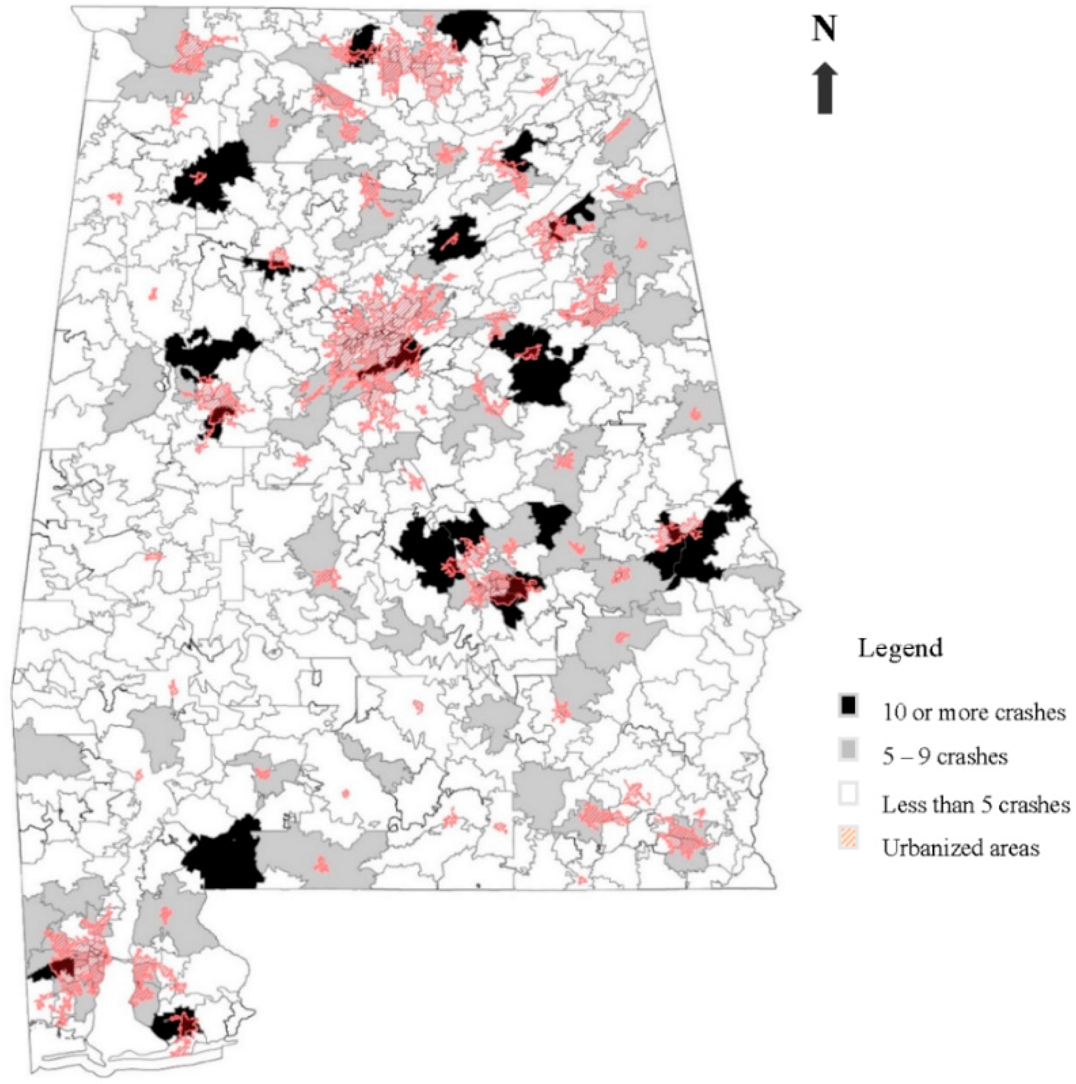
Figure 1 shows where young drivers that caused crashes close-to-home live (based on the postal code of the causal driver from the crash report).
In
Figure 1, the postal codes that are colored black indicate that ten or more drivers from that postal code caused a close-to-home crash over the study period. Postal codes colored grey indicate that 5–9 drivers caused close-to-home crashes, and white postal codes indicate that less than five caused close-to-home crashes. Finally, the areas marked in red hatching show the boundaries of the urbanized areas as designated by the U.S. Census Bureau [
45].
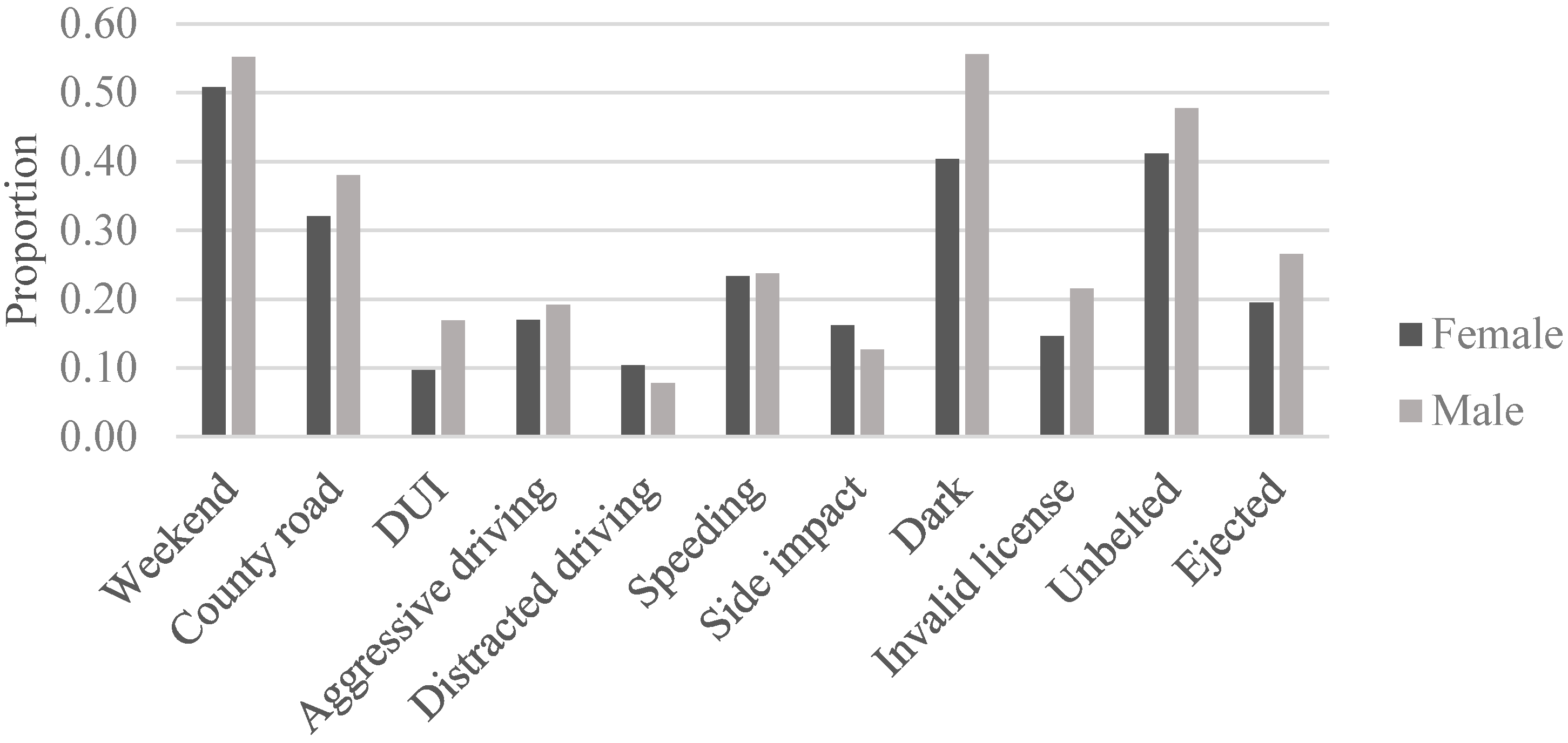
Figure 2 provides a comparison of the risky driving behaviors among male and female young drivers.
Figure 2 shows that, while more fatal crashes are caused by young male drivers than young female drivers (
Table 1), the proportions of total fatal crashes due to speeding and aggressive driving are similar for male and female drivers.
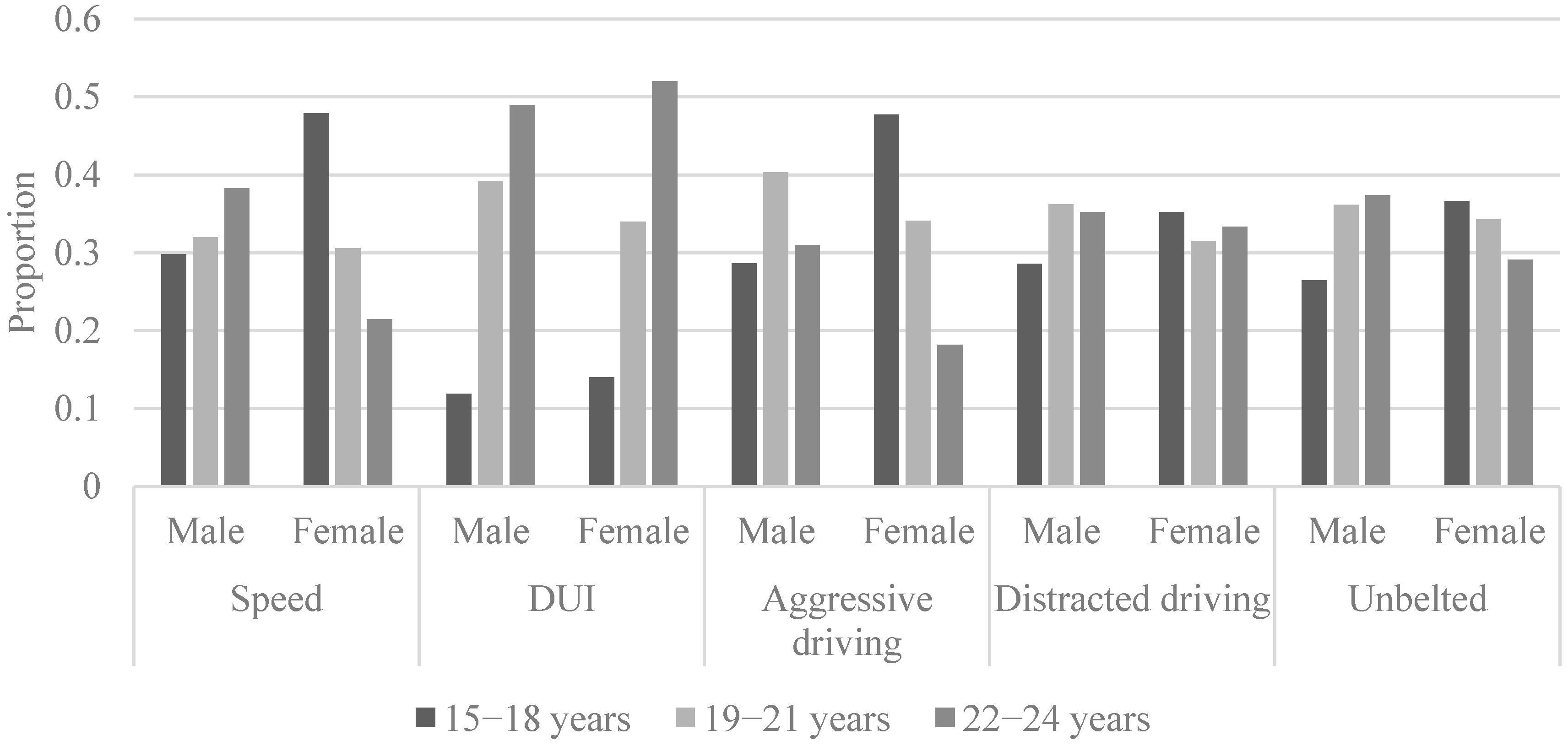
Figure 3 shows a further breakdown of the gendered driving behaviors by subgroups of younger drivers.
Interestingly,
Figure 3 shows very different contributions of speeding to fatal crashes between male and female young drivers—the proportion involving speeding increasing with age for males and decreasing with age for females. In general, younger female drivers (15–18 years) were more likely to be involved in speed and aggressive driving related fatal crashes than their male counterparts. Fatal crashes involving DUI increase with age for both male and female drivers, with a significant increase for drivers between 19 and 21 years of age, perhaps concurrent with the legal drinking age of 21. The proportions of fatal crashes that are attributable to distracted driving or not wearing a seat belt were similar for both males and females across the age groups.
3. Methodology
Latent class analysis (LCA) is a widely used model-based clustering method for identifying a set of subgroups of individuals based on the intersection of multiple observed characteristics [
46,
47,
48,
49,
50]. In other words, LCA is based on the assumption that there is an underlying unobserved categorical variable that divides a population into mutually exclusive and exhaustive latent classes. The modeling technique therefore assumes that each observation of heterogeneous data comes from one of a number of classes and models each with its own probability distribution [
51,
52]. The overall population therefore follows a finite mixture model, given as:
where
f is the density for latent class
c,
C is the number of classes,
πc are the mixture proportions, 0 < π
c < 1, and
,
and
are the set of parameters for the class.
In LCA, the variables are assumed to be independent, given knowledge of the class that an observation came from. Each variable within each latent class is then modeled with a multinomial density. So, given
k variables, the joint class density can be expressed as a product of the individual class densities. Given that
x = (
x1, …,
xk), the joint class density is expressed as:
where
is the indicator function equal to 1 if the observation of the
ith variable takes value
j and 0; otherwise,
pijc is the probability of the variable
i taking a value
j in class
c, and
di is the number of possible values or categories the
ith variable can take. The overall density is then a weighted sum of these individual densities, given by:
The model parameters
pijc and
πc can be estimated from the data (for a fixed value of C) by maximum likelihood using the expectation-maximization algorithm or the Newton-Raphson algorithm, or a hybrid of the two [
47].
Model selection in LCA can be done either by considering the absolute fit of a particular model or the relative fit of two or more competing models. The
G2 likelihood-ratio Chi-square statistic is a common measure of absolute model fit in categorical models. This tests the null hypothesis that the specified LCA model fits the data [
53]. This statistic has an asymptotic Chi-square distribution; thus, when the sample size is sufficient and the degrees of freedom are not too large, this value can be compared to the Chi-square distribution with degrees of freedom given by the LCA model. Information criteria (e.g., Akaike Information Criterion (AIC), Bayesian Information Criterion (BIC), Consistent Akaike Information Criterion (CAIC)) can be used to compare the relative fit of the models with different numbers of latent classes. For all of these information criteria, a lower value suggests a more optimal balance between model fit and parsimony. For this study, the LCA models were estimated using the PROC LCA procedure in SAS (Version 9.4, SAS Institute Inc., Cary, NC, USA).
4. Results
To account for measurement invariance, two nested, multi-group LCA procedures were conducted to compare the freely estimated model with a model where measurement parameter estimation was restricted across groups (i.e., for male and female drivers). This was done by comparing
G2 the difference of these models to a Chi-square distribution with degrees of freedom equal to the difference in degrees of freedom between the models [
54]. The analyses conducted for this study indicated that measurement invariance should be rejected (
p < 0.001) and that males and females should be estimated separately.
LCA was applied to identify nine distinct classes of fatal crash risk factors for both young male and female drivers, as summarized by the fit statistics reported in
Table 2 and
Table 3. No significant improvements in model performance were observed beyond the nine classes. Both nine-class models also exhibited good separation among classes, as indicated by the entropy criterion, where entropy criterion of one (1.0) indicates perfect classification [
51].
Table 4 and
Table 5 show the probabilities of the various fatal crash factors contributing to each class for males and females, respectively.
The probabilities in each were examined to ascertain what factors seemed to define each class. In doing so, the probabilities of a given factor belonging to a certain class were inspected with the understanding that a factor with a higher probability (i.e., closer to 1.000) indicated its relative contribution to the percent of total fatal crashes that were captured in that latent class. For example, Class 2 in the male results (
Table 4) accounted for roughly 4% of fatal crashes that were attributable to male drivers. This class appears to be defined by all single-vehicle crashes (probability = 1.000), all involving distracted driving (probability = 1.000) that occurred in a rural area (probability = 0.903). By similar logic, Class 6 within the female drivers’ results (
Table 5) appear to be defined by side impact crashes (probability = 0.948) occurring at intersections (probability = 0.841) involving aggressive driving (probability = 0.889), which might suggest running red-lights, stops signs, or other traffic control devices.
No formal rubric was applied to the probability values in defining each class. Rather, the categorization of each class was conducted through the inspection of the probabilities which was informed by an understanding of the data and the context of crashes in Alabama.
Table 6, then, presents a summary for all nine classes for both males and females. Inspection of
Table 6 allows comparisons among different classes (representing different proportions of fatal crashes) within each gender, as well as contrasts between the factors that are driving the fatal crashes that are attributable to young male versus young female drivers.
As indicated in
Table 1, a little over half of young driver crashes occurred at night and
Figure 1 shows that a higher proportion of male drivers crashed during dark conditions than female drivers. The classes that are summarized in
Table 6 provide further insight by suggesting that these nighttime crashes often occurred on rural two-lane roads and involved a risky driving behavior such as speeding, DUI, or distracted driving. While night crashes appear to be less prominent among young female drivers, Classes 5 and 9 suggest that these were single-vehicle events involving DUI or distracted driving.
Class 1 comprised the most fatal crashes that were attributable to young male drivers (17%) on two-lane rural roads during weekend nights. Whereas, Class 7 represented the largest proportion (21%) of fatal crashes that were attributable to young female drivers and involved only one vehicle and an unbelted driver—less than half of which occurred at night. Class 9 for young female drivers was similar to Class 7, adding another 13% of such crashes, but emphasizing their rural nature. Interestingly, 5% of fatal crashes that were attributable to young females involved drivers without a valid license (Class 2), but no such finding was present for male drivers.
There are also similarities between the genders. For example, Class 3 for both males and females each accounts for 12% of fatal crashes that are attributable to young drivers that are characterized as single-vehicle crashes on rural roads occurring close-to-home involving speeding. Interestingly, the Class 3 drivers also involved a high percentage of unbelted drivers. Class 6 for both male and female young drivers indicates the danger of aggressive driving as it likely relates to adherence to traffic control devices. And finally, it is worth noting that accounting for race among young drivers simply reflected the fact that Caucasian drivers represent the overwhelming majority of young drivers (
Table 1) and in such a way as to be representative of the general population in Alabama [
45] and consistent with previous findings [
55].
5. Discussion
Every study has certain limitations regarding data quality or the methodology used. However, since this study is based only on fatal crashes, under-reporting is highly unlikely given the diligence with which such data is handled in the U.S. Even with the limitations underlying LCA methodology, this study presents interesting findings on young driver fatal crashes in Alabama, USA.
To be able to implement human-centered crash countermeasures, it is important to identify the characteristics of the at-risk population and how to best select, plan, and implement effective and efficient countermeasures. Clearly, this study has revealed that crashes on rural roads are a serious issue in Alabama. Indeed, in the ten years from 2007 to 2016, rural crashes consistently accounted for roughly 60% of all road fatalities in Alabama where less than half of the population live in rural areas [
45]. However, while it is likely that a crash occurring in a rural area ends in a fatal outcome, in some instances this might be related to response time and the availability/quality of emergency care [
56,
57].
Table 6 clearly shows the contribution of different young driver behaviors to fatal crashes in the rural context. It should also be noted, however, that some researchers have explicitly noted the roadway environment itself as influencing younger drivers’ behaviors and crashes—for example, [
58] it has linked road sinuosity to differences in crashes between young male and female drivers. On the other hand, Cox et al. [
59] reported no difference among the relative perception of risks between urban and rural roadway environments for younger drivers.
Figure 1, in conjunction with
Table 6, suggests that many of the young drivers who are involved in fatal crashes are from rural homes. This is an interesting point in that these crashes are attributable to specific risky behaviors that are exhibited by these young drivers from rural areas. The data and results indicate that the majority of younger driver crashes in Alabama are single-vehicle crashes that are attributable to one (or more) of three risky driving behaviors: distracted driving, aggressive driving, and/or driving under the influence. And the instance of unbelted drivers further contributes to the increased severity of these crashes.
Previous research has established relationships among increased propensity of fatal crashes, low population densities, and socioeconomic deprivation [
55,
60,
61,
62,
63,
64,
65,
66,
67,
68,
69,
70,
71]. More pointedly, a longitudinal study concluded that young drivers that are associated with lower socioeconomic opportunity (particularly educational) were more likely to be involved in serious crashes, especially single-vehicle crashes [
72]. Such conditions are certainly representative across many rural areas throughout Alabama and elsewhere. For example, a suite of nine spatial econometric models of relationships among socioeconomic factors and DUI crashes in Alabama all indicated that educational attainment and income levels for an individual postal code significantly contributed to lower rates of DUI crashes among the residents from that postal code. Further, seven of the nine models also indicated that DUI crash rates among residents of a given postal code were lower among more urbanized areas, as measured by the percentage of rental households in each postal code [
73]. The relationships were further supported by Geographic Weighted Poisson Regression analysis of socioeconomic factors affecting DUI crashes in Alabama [
74]. Some of the postal codes in
Figure 3 indicating higher instances of fatal crashes among younger drivers overlap or are in the vicinity of urbanized areas. Material deprivation (i.e., socioeconomic opportunity) is often as or more associated with risky driving behaviors among youths in urban and suburban locations as well [
75].
Overall, the results reported here reinforce previous studies, highlighting the characteristics of young driver crashes. For example, in New Zealand, there has been an indication that high speeds, alcohol, lack of seat belt use, and nighttime conditions on rural roads are significant contributors of fatal crashes among young drivers [
76]. Even the role weekend travel plays in these crashes is supported elsewhere in the literature [
20,
77] and specifically in the case of Alabama [
55,
56,
57,
58,
59,
60,
61,
62,
63,
64,
65,
66,
67,
68,
69,
70,
71,
72,
73,
74,
75,
76,
77,
78].


