
Aerodynamic Analysis of Camber Morphing Airfoils in Transition via Computational Fluid Dynamics


Abstract
:1. Introduction
2. Methodology
3. Modeling Approach and Mathematical Background
3.1. Assumption
- Air Properties
- Density: 1
- Viscosity μ:
- Far-field pressure:
- Geometry Properties
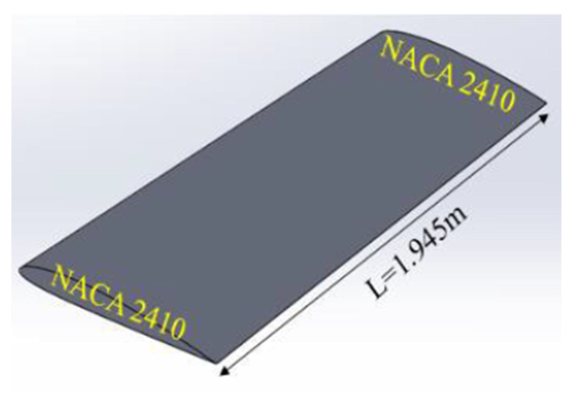
- Some of the geometrical explanation for the airfoil is shown in Figure 1 below.
- Wingspan:
- Chord length:
- Re:
- where
3.2. Geometry
3.2.1. NACA Four-Digit Airfoil Specification
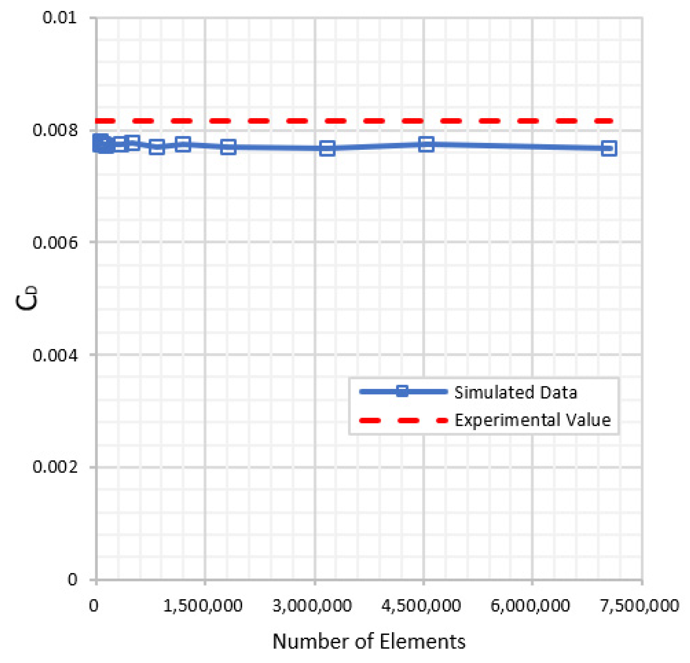
3.2.2. Meshing
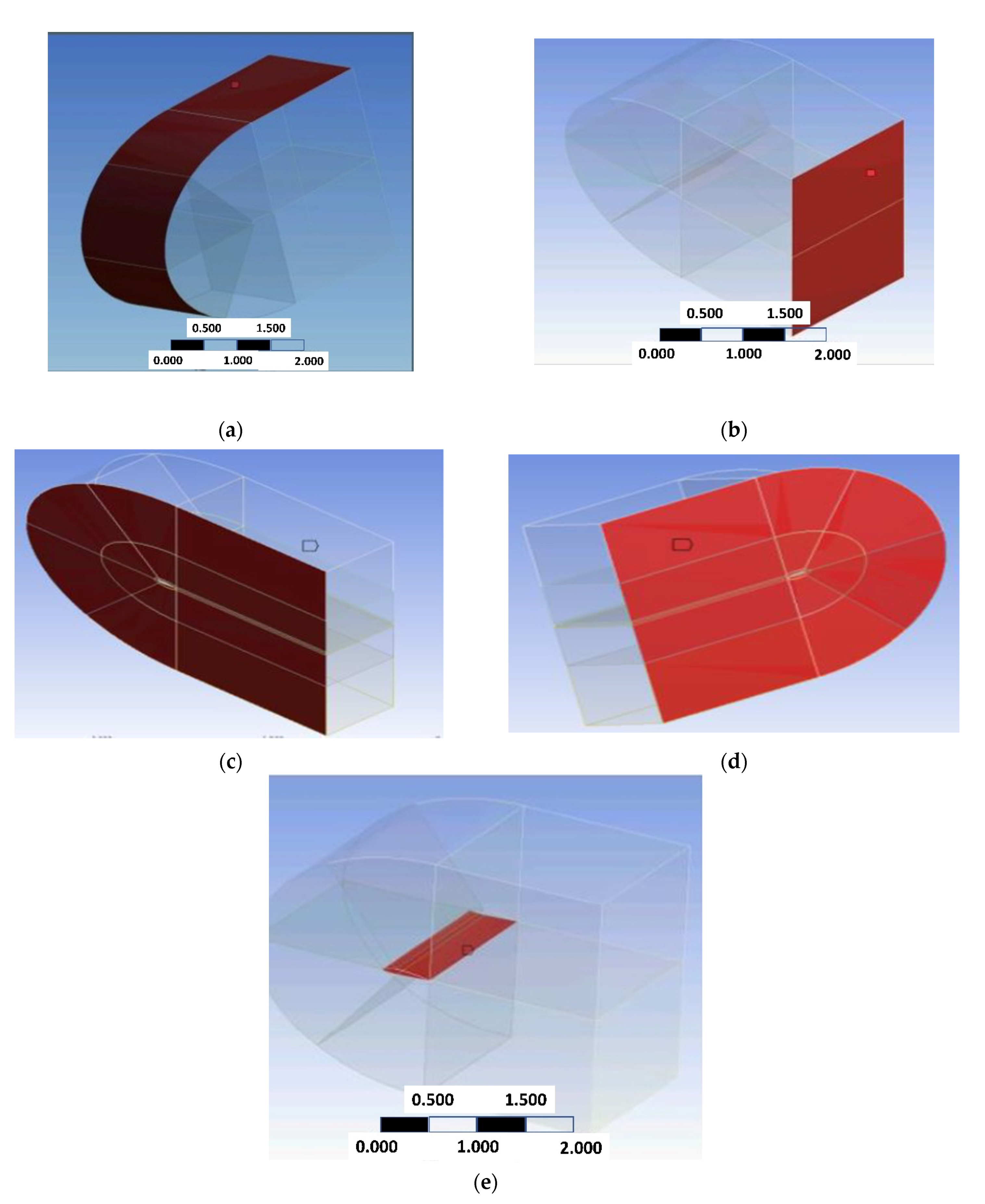
3.2.3. Boundary Conditions
- (1)
- The inlet equals a velocity inlet,
- (2)
- The outlet equals a pressure outlet,
- (3)
- Faces with wing ends are symmetric, and
- (4)
- No-slip condition on the wall.
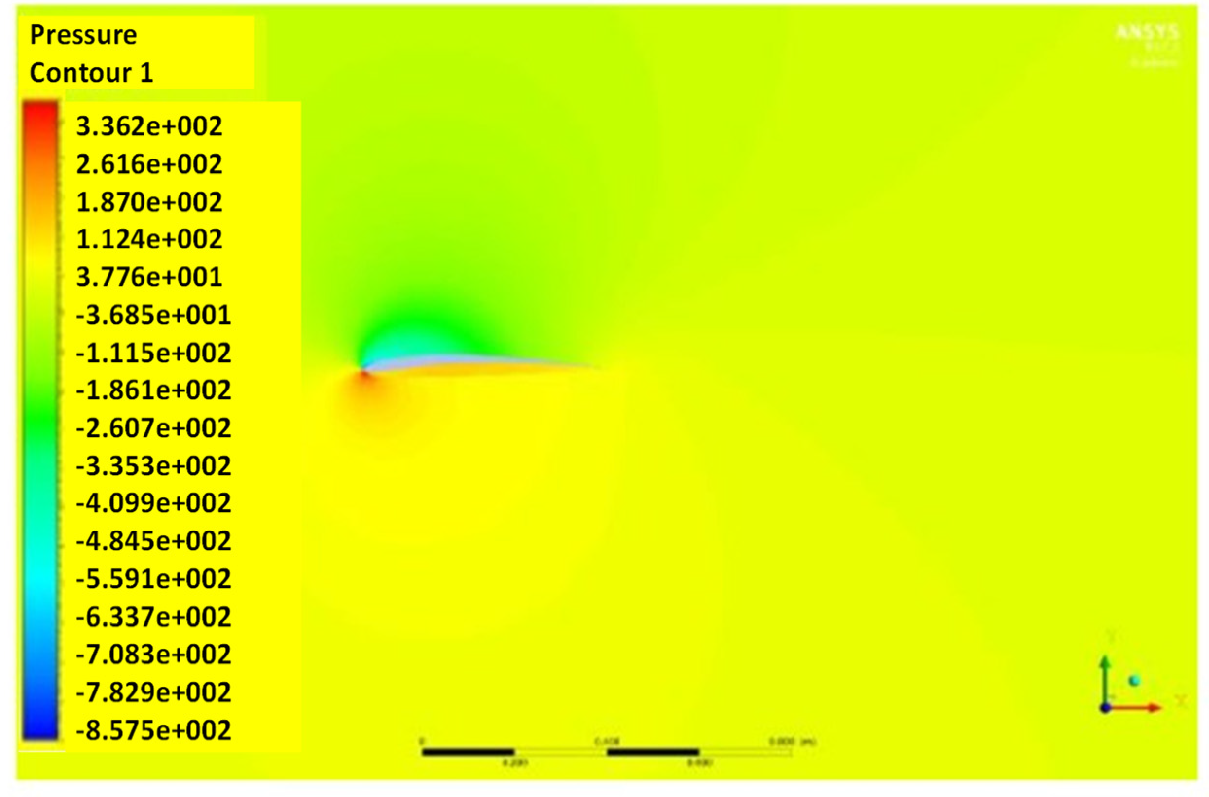
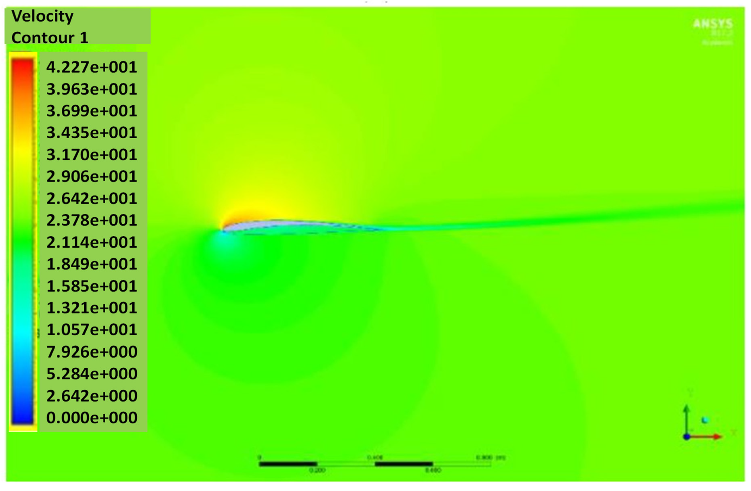
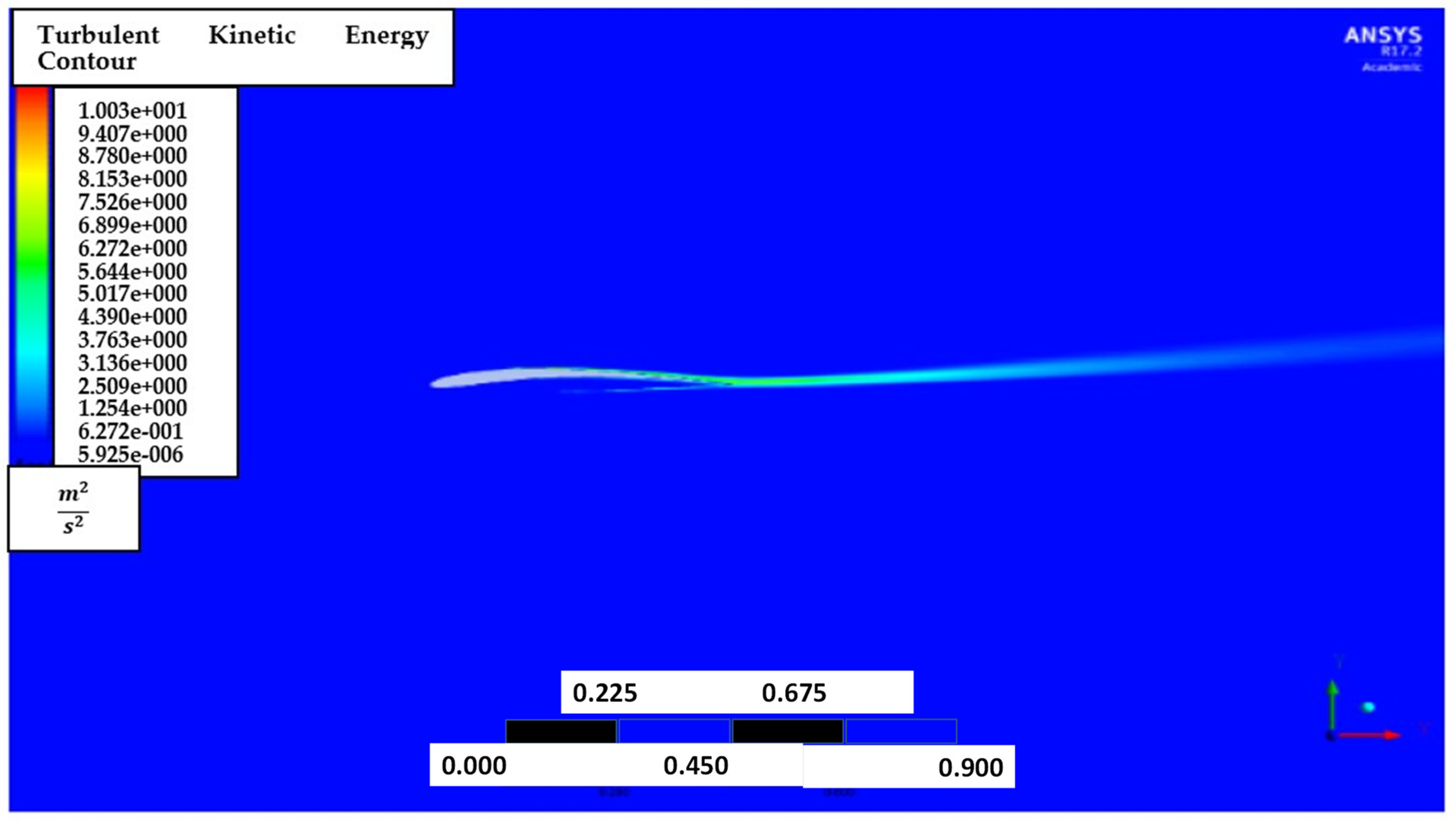
4. Result
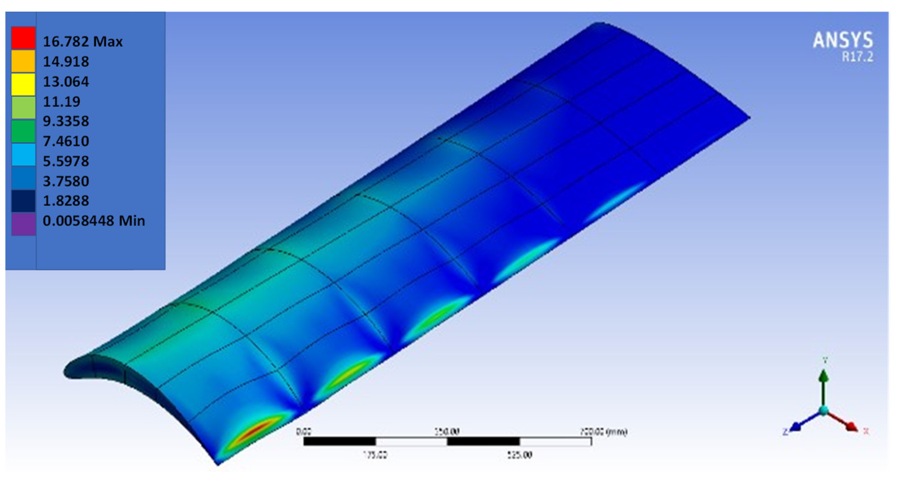
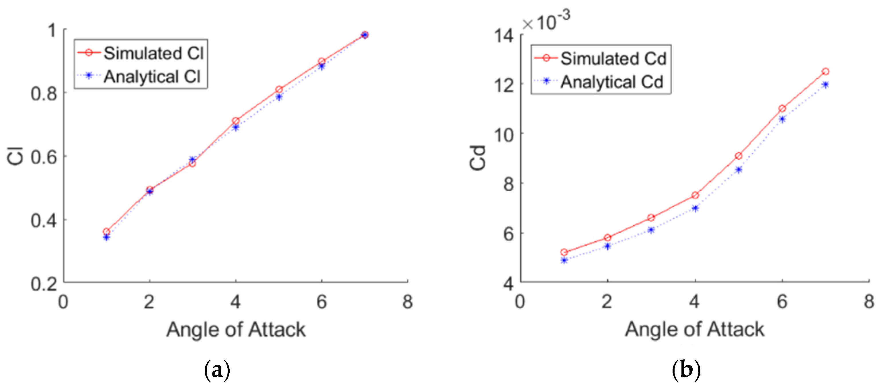
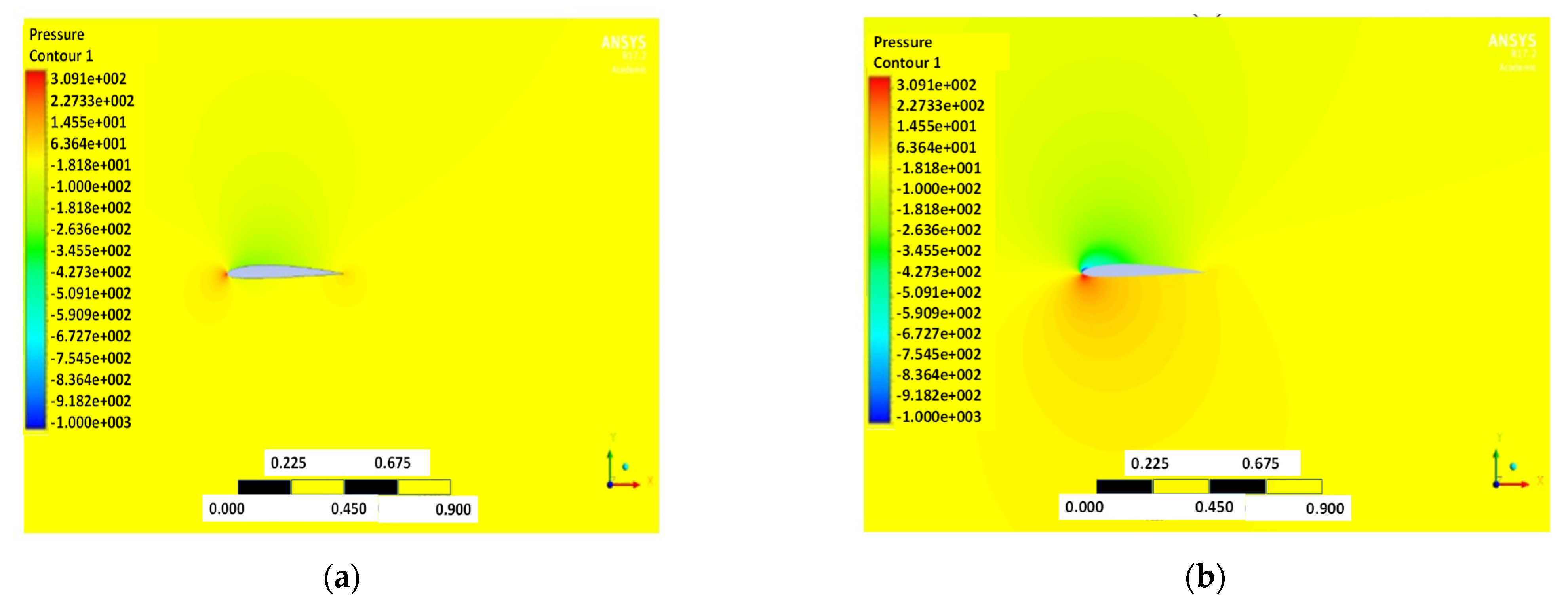
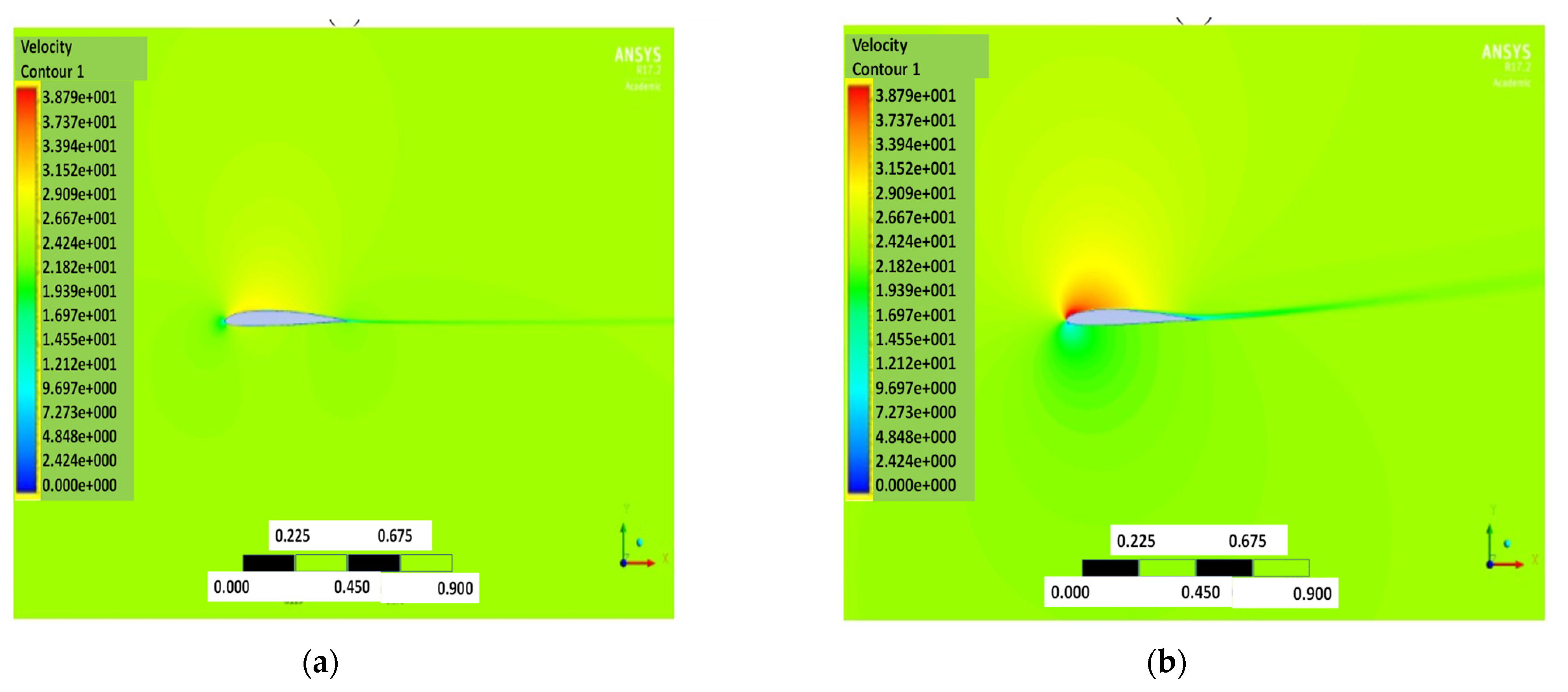
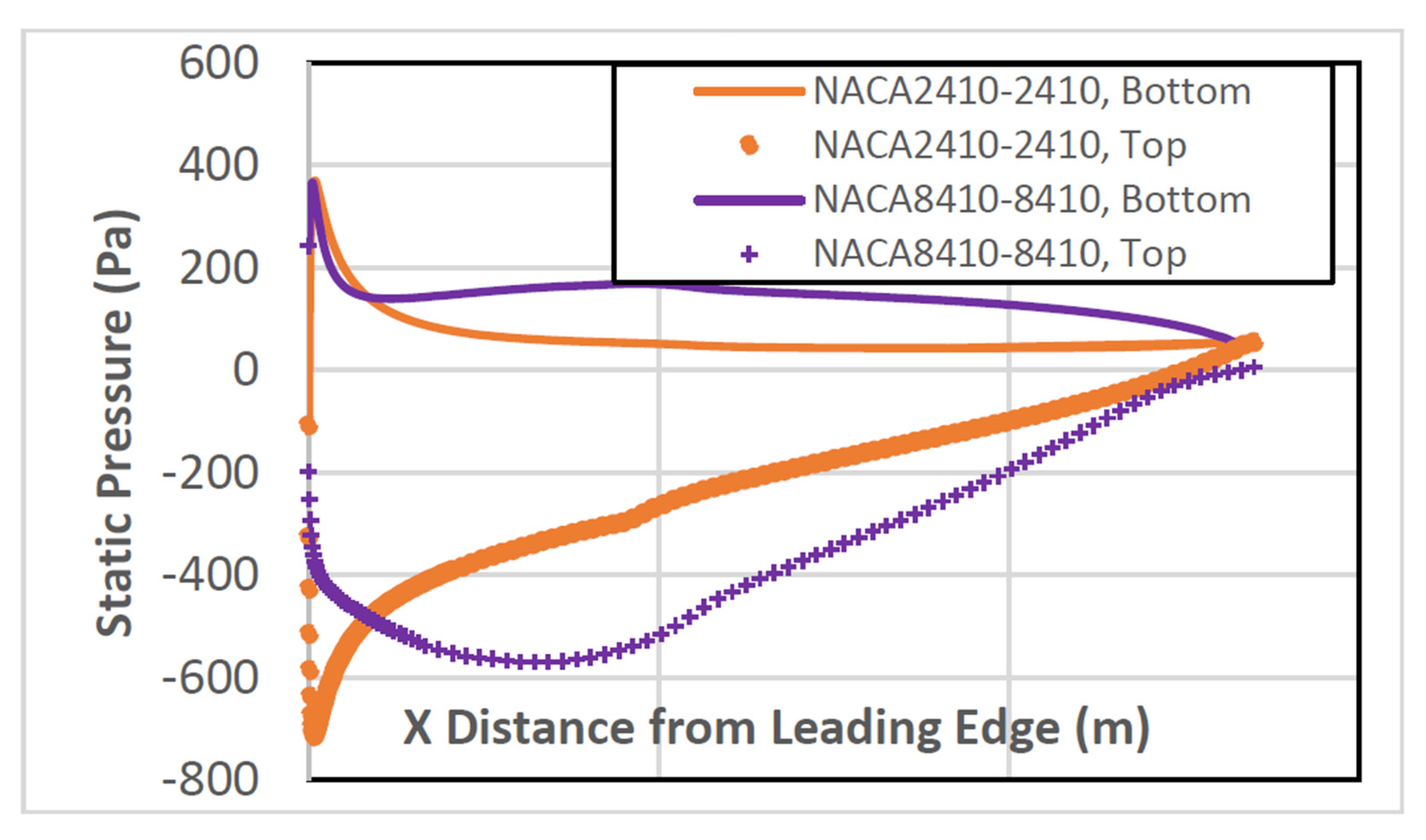
4.1. NACA2410
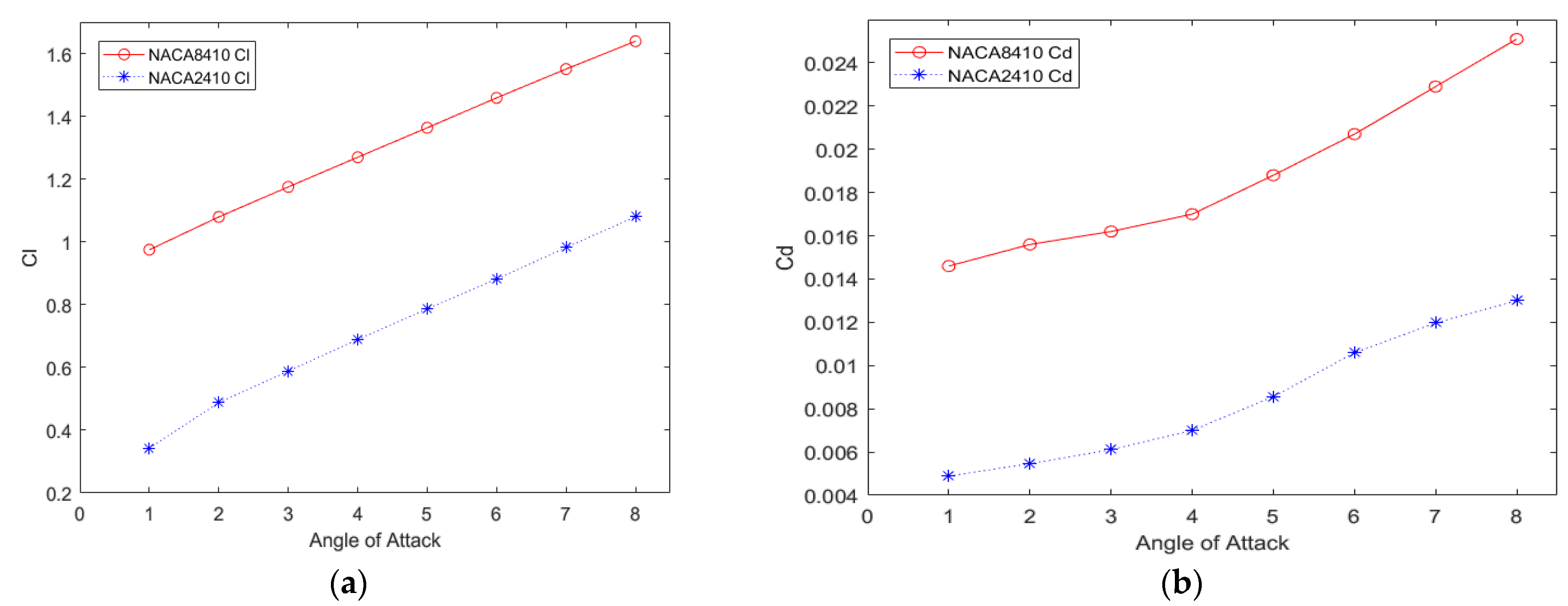
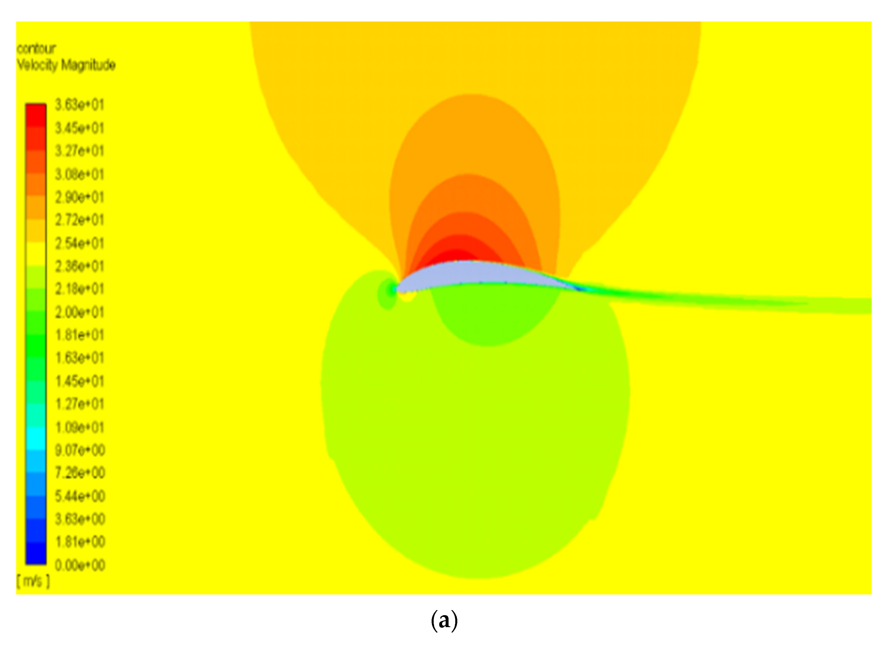
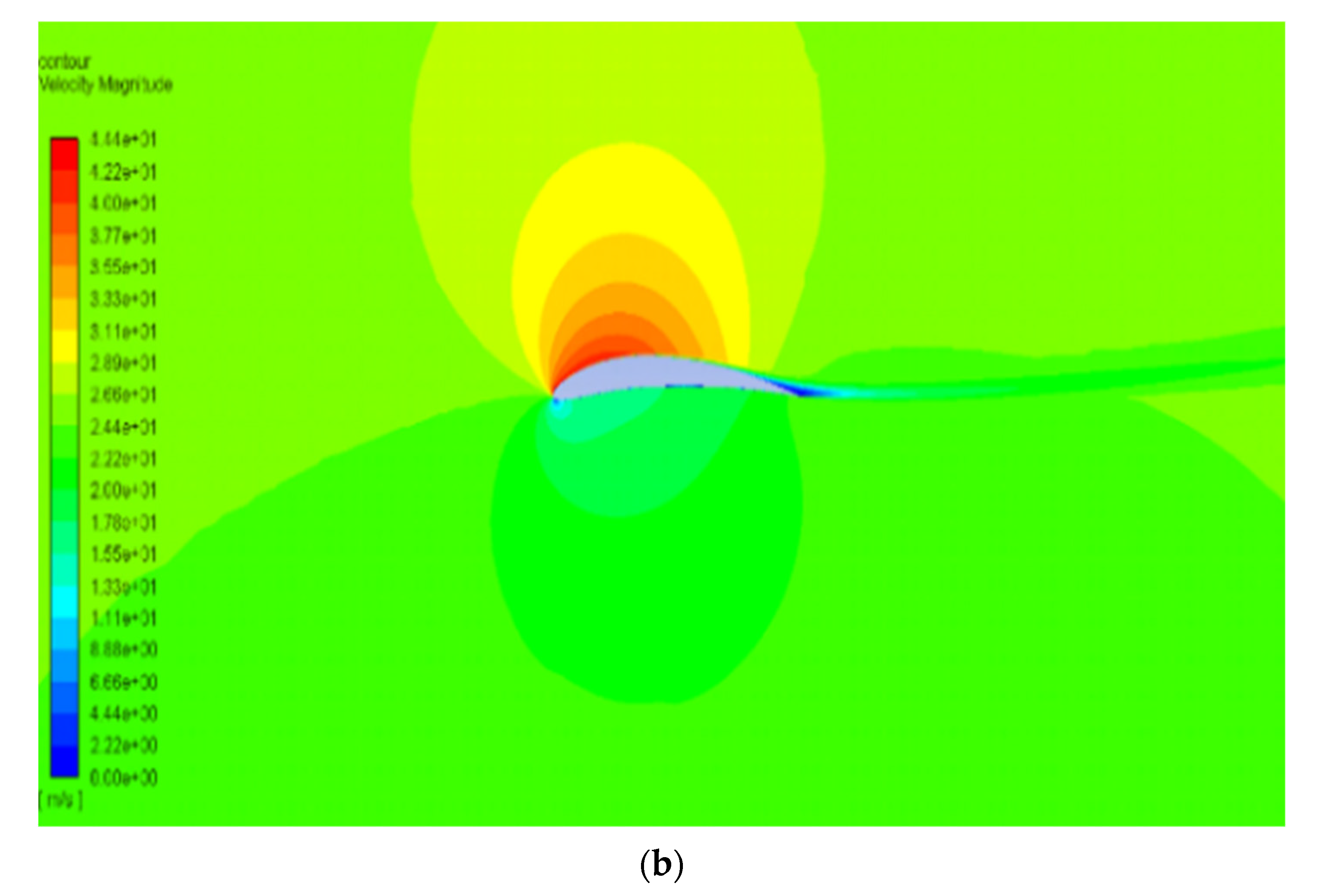
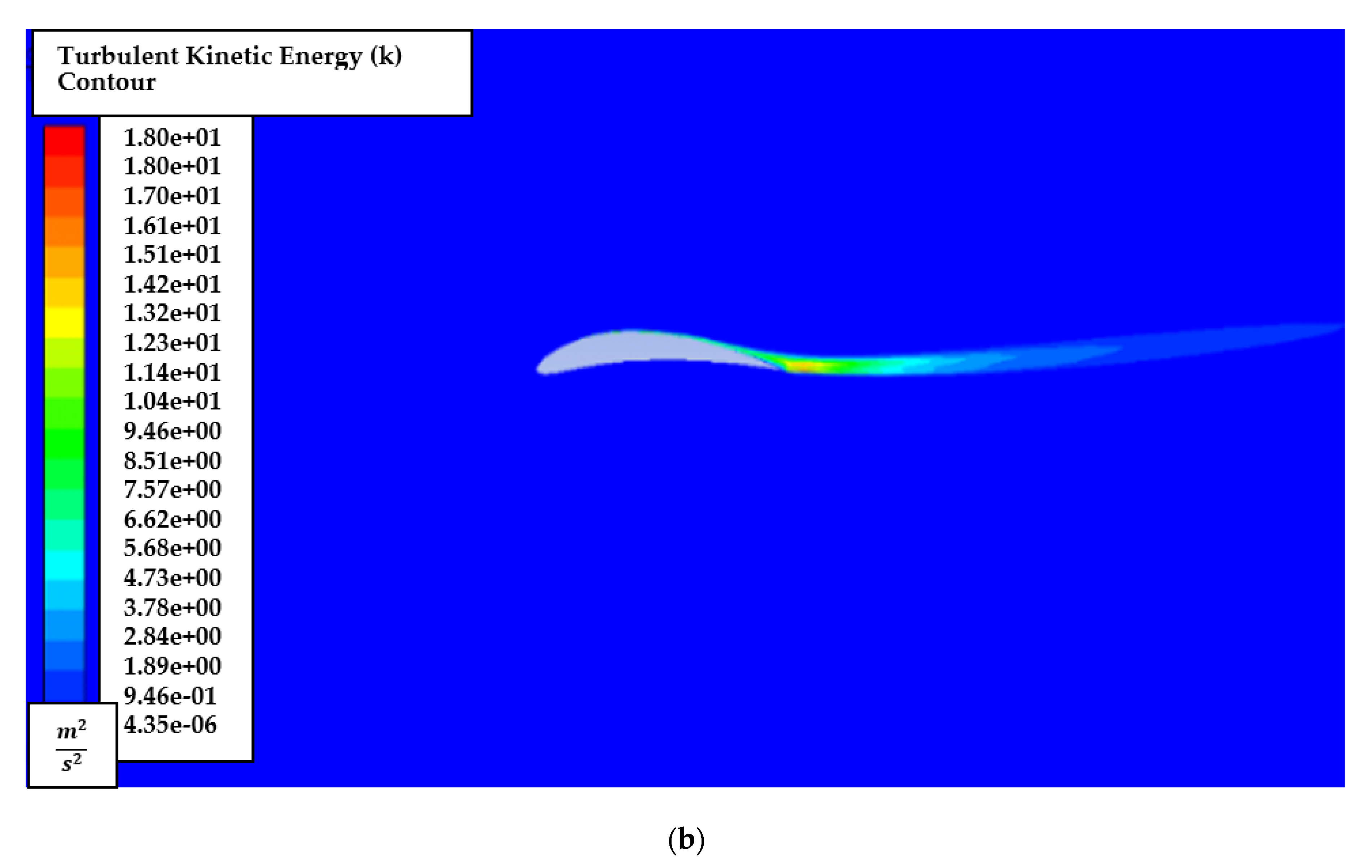
4.2. NACA8410
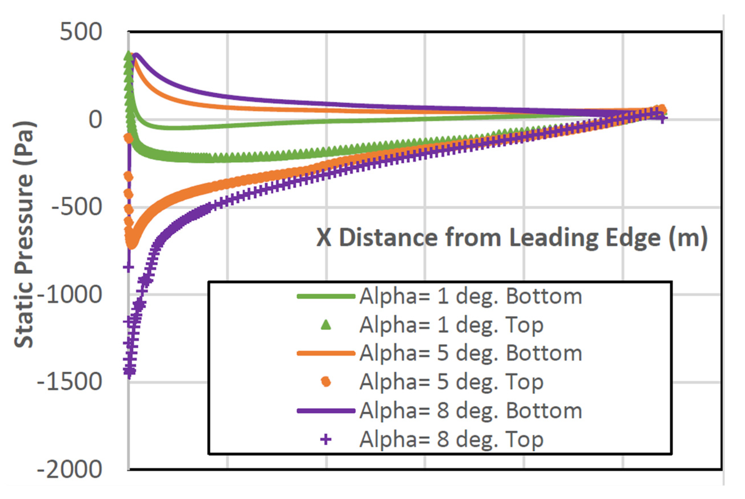
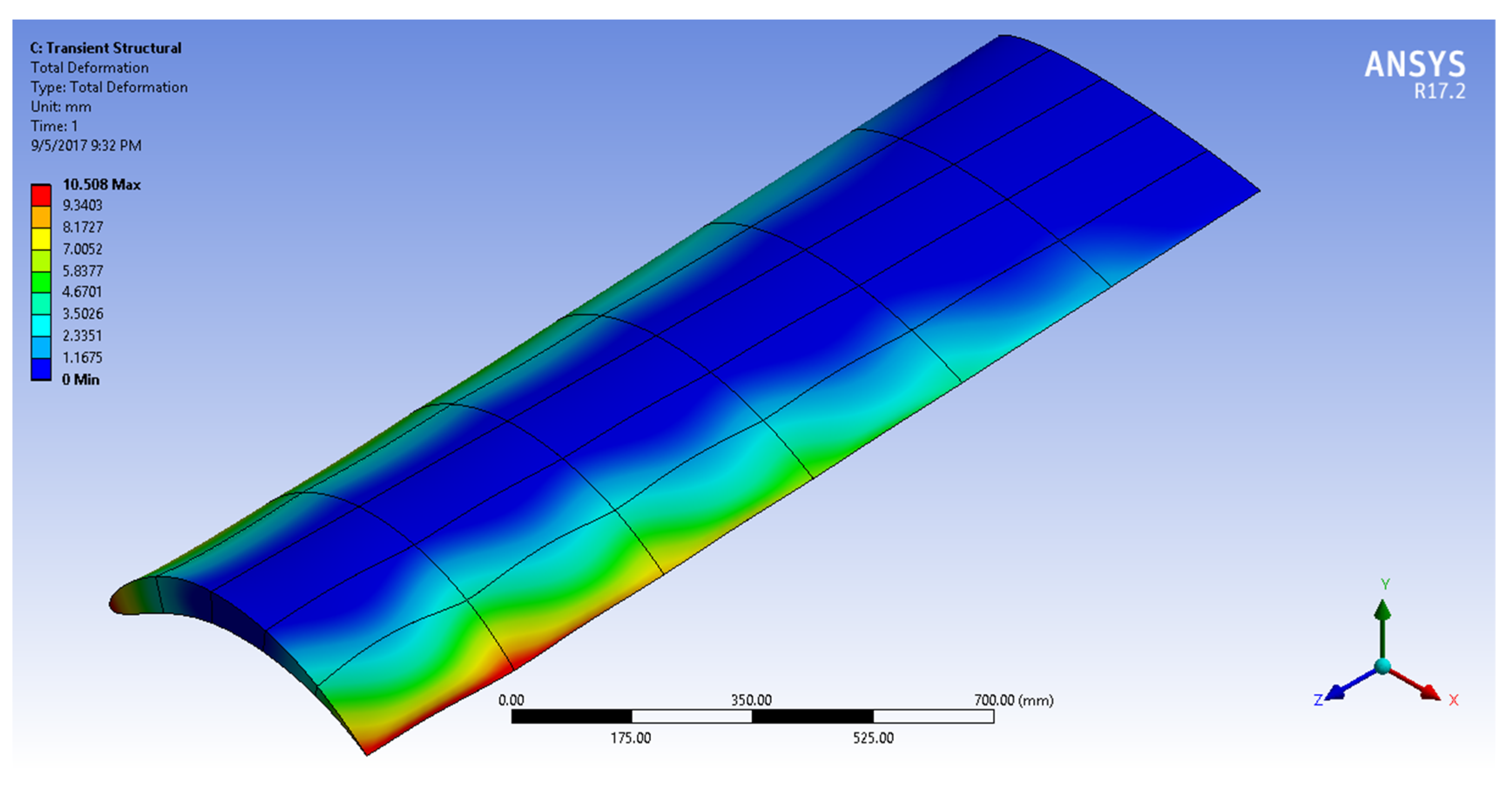
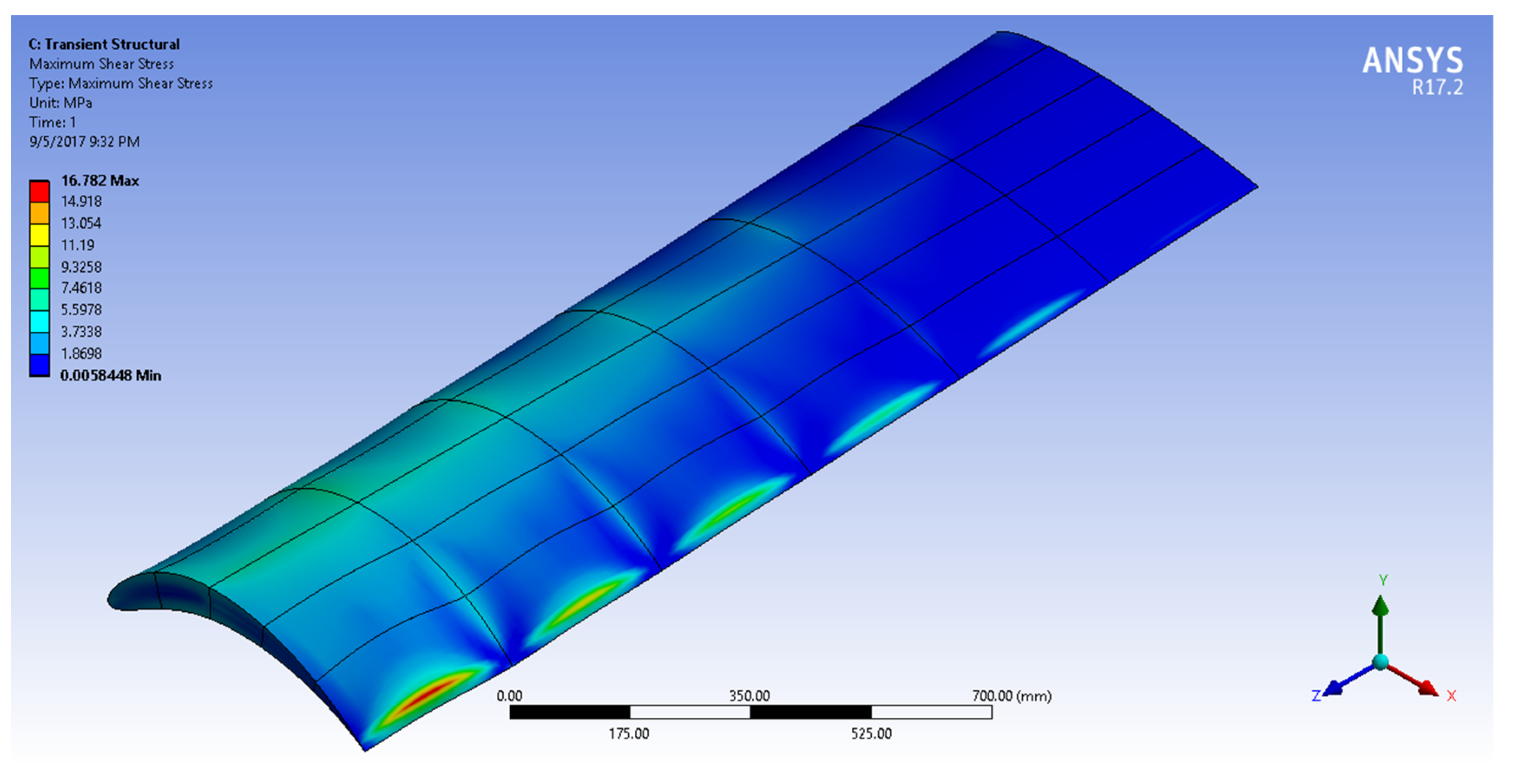
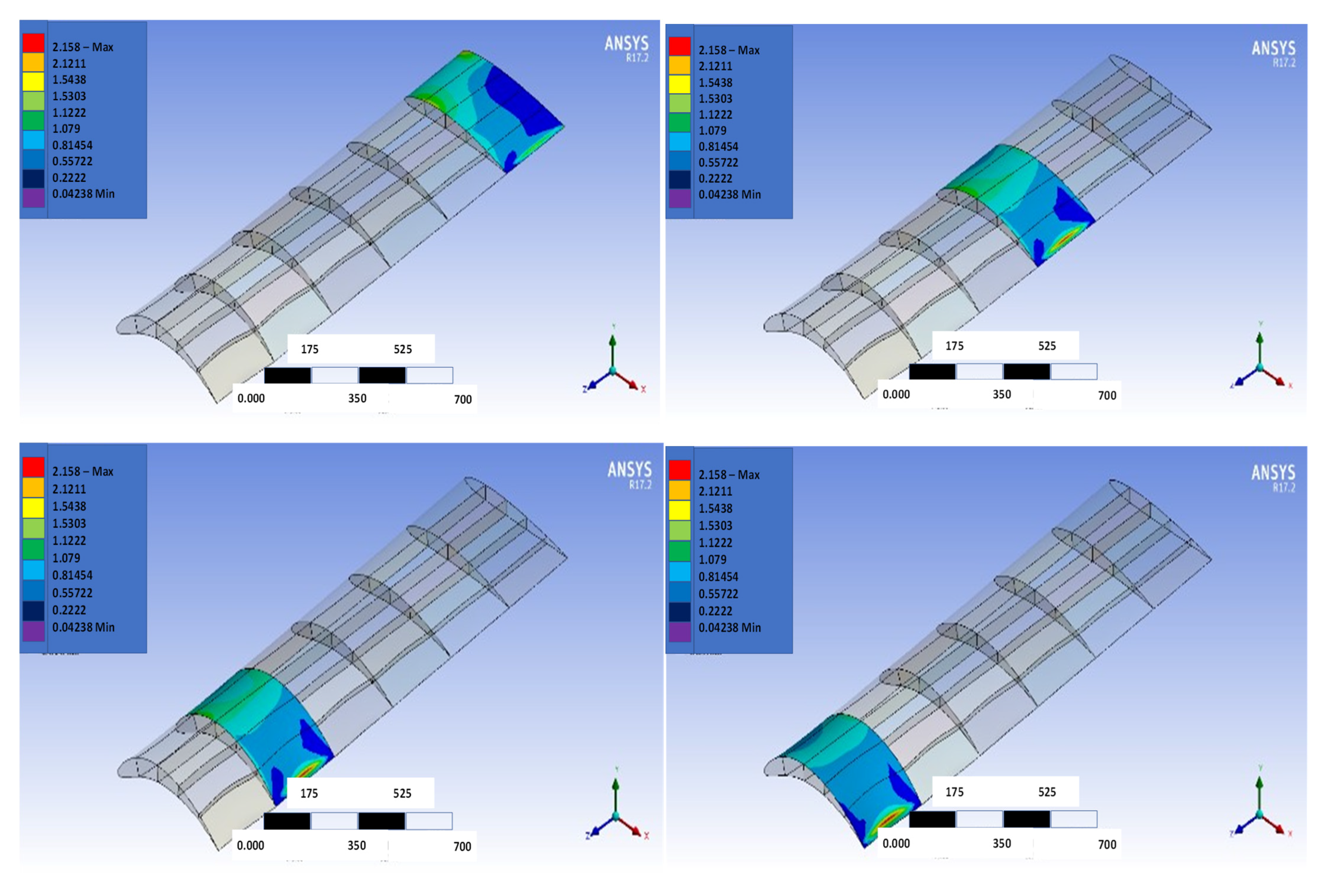
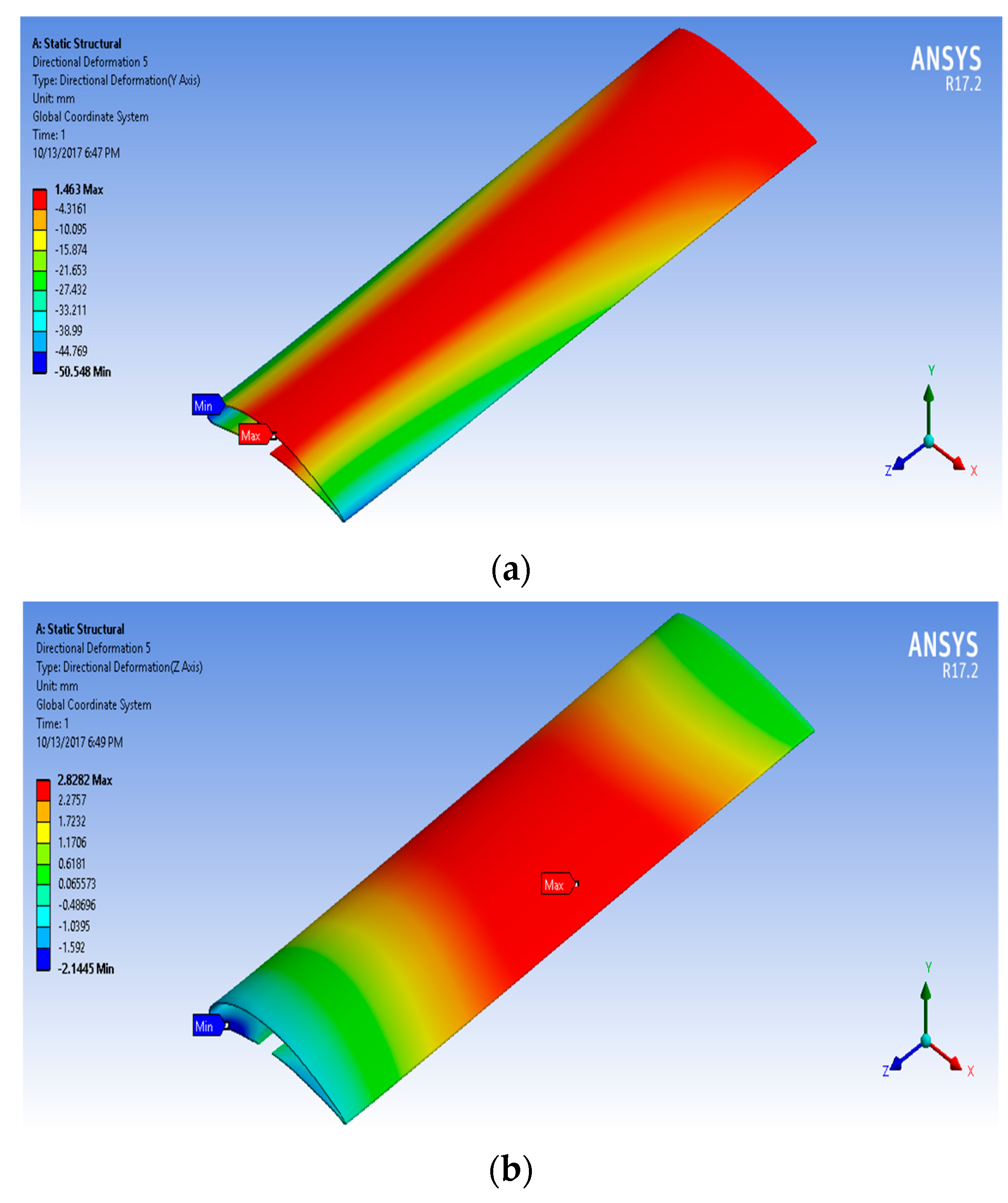
4.3. From NACA2410 to NACA8410 Transition
5. Summary
6. Conclusions
Author Contributions
Funding
Institutional Review Board Statement
Informed Consent Statement
Data Availability Statement
Acknowledgments
Conflicts of Interest
Nomenclature
| L | lift force |
| D | drag force |
| CL | lift coefficient |
| DL | drag coefficient |
| AoA | angle of attack |
| Cf | skin friction coefficient |
| k | turbulent kinetic energy |
| distance between airfoil wall and first layer | |
| Greek Symbols | |
| μ | viscosity |
| ρ | density of air |
| wall shear stress | |
| ω | dissipation of a specific turbulent |
Abbreviations
| CFD | computational fluid dynamics |
| RANS | Reynold’s-averaged Navier–Stokes |
| RST | Reynold’s stress transport |
| RSM | Reynold’s stress models |
| EWT | enhanced wall treatment |
| TBL | turbulent boundary layer |
| VBL | viscous boundary layer |
| IT/CC | intermittency transition/curvature correction |
| SST | shear stress transport |
| NACA | National Advisory Committee for Aeronautics |
References
- Miller, G.D. Active Flexible Wing (AFW) Technology; Rockwell International Los Angeles Ca North American Aircraft Operations: Fort Belvoir, VA, USA, 1988. [Google Scholar]
- Anderson, J.D.; Bowden, M.L. Introduction to Flight; Mc Graw Hill: New York, NY, USA, 2005. [Google Scholar]
- Barbarino, S.; Bilgen, O.; Ajaj, R.M.; Friswell, M.I.; Inman, D.J. A review of morphing aircraft. J. Intell. Mater. Syst. Struct. 2011, 22, 823–877. [Google Scholar] [CrossRef]
- Martin, C.; Kudva, J.; Austin, F.; Jardine, A.; Scherer, L.; Lockyer, A.; Carpenter, B. Smart Materials and Structures-Smart Wing Volumes I, II, III, and IV; Report: AFRL-ML-WP-TR-1999-4162; Northrop Grumman Corporation: Hawthorne, CA, USA, 1998. [Google Scholar]
- Weisshaar, T.A. Morphing Aircraft Technology-New Shapes for Aircraft Design; Defense Technical Information Center: Fort Belvoir, VA, USA, 2006. [Google Scholar]
- Bhushan, B. Biomimetics: Lessons from nature—An overview. Philos. Trans. R. Soc. A Math. Phys. Eng. Sci. 2009, 367, 1445–1486. [Google Scholar] [CrossRef] [Green Version]
- Bye, D.; McClure, P. Design of a morphing vehicle. In Proceedings of the 48th AIAA/ASME/ASCE/AHS/ASC Structures, Structural Dynamics, and Materials Conference, Honolulu, HI, USA, 23–26 April 2007; p. 1728. [Google Scholar]
- Kudva, J.N. Overview of the DARPA smart wing project. J. Intell. Mater. Syst. Struct. 2004, 15, 261–267. [Google Scholar] [CrossRef]
- Sofla, A.; Meguid, S.; Tan, K.; Yeo, W. Shape morphing of aircraft wing: Status and challenges. Mater. Des. 2010, 31, 1284–1292. [Google Scholar] [CrossRef]
- Sun, J.; Guan, Q.; Liu, Y.; Leng, J. Morphing aircraft based on smart materials and structures: A state-of-the-art review. J. Intell. Mater. Syst. Struct. 2016, 27, 2289–2312. [Google Scholar] [CrossRef]
- Abdulrahim, M.; Lind, R. Flight testing and response characteristics of a variable gull-wing morphing aircraft. In Proceedings of the AIAA Guidance, Navigation, and Control Conference and Exhibit, Providence, RI, USA, 16–19 August 2004; p. 5113. [Google Scholar]
- Alulema, V.H.; Valencia, E.A.; Pillajo, D.; Jacome, M.; Lopez, J.; Ayala, B. Degree of Deformation and Power Consumption of Compliant and Rigid-linked Mechanisms for Variable-Camber Morphing Wing UAVs. In Proceedings of the AIAA Propulsion and Energy 2020 Forum, Online, 24–28 August 2020; p. 3958. [Google Scholar]
- Basaeri, H.; Yousefi-Koma, A.; Zakerzadeh, M.R.; Mohtasebi, S.S. Experimental study of a bio-inspired robotic morphing wing mechanism actuated by shape memory alloy wires. Mechatronics 2014, 24, 1231–1241. [Google Scholar] [CrossRef]
- Bilgen, O.; Kochersberger, K.; Inman, D.J. Macro-fiber composite actuators for a swept wing unmanned aircraft. Aeronaut. J. 2009, 113, 385–395. [Google Scholar] [CrossRef] [Green Version]
- Bishay, P.L.; Finden, R.; Recinos, S.; Alas, C.; Lopez, E.; Aslanpour, D.; Flores, D.; Gonzalez, E. Development of an SMA-based camber morphing UAV tail core design. Smart Mater. Struct. 2019, 28, 075024. [Google Scholar] [CrossRef]
- Campanile, L.; Sachau, D. The belt-rib concept: A structronic approach to variable camber. J. Intell. Mater. Syst. Struct. 2000, 11, 215–224. [Google Scholar] [CrossRef]
- Chanzy, Q.; Keane, A. Analysis and experimental validation of morphing UAV wings. Aeronaut. J. 2018, 122, 390–408. [Google Scholar] [CrossRef] [Green Version]
- Communier, D.; Botez, R.M.; Wong, T. Design and Validation of a New Morphing Camber System by Testing in the Price—Païdoussis Subsonic Wind Tunnel. Aerospace 2020, 7, 23. [Google Scholar] [CrossRef] [Green Version]
- Fasel, U.; Keidel, D.; Baumann, L.; Cavolina, G.; Eichenhofer, M.; Ermanni, P. Composite additive manufacturing of morphing aerospace structures. Manuf. Lett. 2020, 23, 85–88. [Google Scholar] [CrossRef]
- Jenett, B.; Calisch, S.; Cellucci, D.; Cramer, N.; Gershenfeld, N.; Swei, S.; Cheung, K.C. Digital morphing wing: Active wing shaping concept using composite lattice-based cellular structures. Soft Robot. 2017, 4, 33–48. [Google Scholar] [CrossRef] [Green Version]
- Kang, W.-R.; Kim, E.-H.; Jeong, M.-S.; Lee, I.; Ahn, S.-M. Morphing wing mechanism using an SMA wire actuator. Int. J. Aeronaut. Space Sci. 2012, 13, 58–63. [Google Scholar] [CrossRef] [Green Version]
- Keidel, D.; Molinari, G.; Ermanni, P. Aero-structural optimization and analysis of a camber-morphing flying wing: Structural and wind tunnel testing. J. Intell. Mater. Syst. Struct. 2019, 30, 908–923. [Google Scholar] [CrossRef]
- Keidel, D.; Sodja, J.; Werter, N.; De Breuker, R.; Ermanni, P. Development and testing of an unconventional morphing wing concept with variable chord and camber. In Proceedings of the 26th International Conference on Adaptive Structures and Technologies, Kobe, Japan, 14–16 October 2015; pp. 1–12. [Google Scholar]
- Kota, S.; Osborn, R.; Ervin, G.; Maric, D.; Flick, P.; Paul, D. Mission adaptive compliant wing–design, fabrication and flight test. In Proceedings of the RTO Applied Vehicle Technology Panel (AVT) Symposium, Evora, Portugal, 20–23 April 2009; p. 18. [Google Scholar]
- Kudva, J.; Scott, M.; Jacob, J.; Smith, S.; Asheghian, L. Development of a novel low stored volume high-altitude wing design. In Proceedings of the 50th AIAA/ASME/ASCE/AHS/ASC Structures, Structural Dynamics, and Materials Conference, Palm Springer, CA, USA, 4–7 May 2009; p. 2146. [Google Scholar]
- Lee, T.; Chopra, I. Wind tunnel test of blade sections with piezoelectric trailing-edge flap mechanism. In Proceedings of the Annual Forum Proceedings-American Helicopter Society, Washington, DC, USA, 9–11 May 2001; 2001; pp. 1912–1923. [Google Scholar]
- Li, H.; Liu, L.; Xiao, T.; Ang, H. Design and simulative experiment of an innovative trailing edge morphing mechanism driven by artificial muscles embedded in skin. Smart Mater. Struct. 2016, 25, 095004. [Google Scholar] [CrossRef]
- Maki, M. Experimental study of a morphing wing configuration with multi-slotted variable-camber mechanism. In Proceedings of the AIAA Atmospheric Flight Mechanics Conference, Washington, DC, USA, 13–17 June 2016; p. 3849. [Google Scholar]
- Manzo, J.; Garcia, E.; Wickenheiser, A.; Horner, G.C. Design of a shape-memory alloy actuated macro-scale morphing aircraft mechanism. In Proceedings of the Smart Structures and Materials 2005: Smart Structures and Integrated Systems, San Diego, CA, USA, 7–10 March 2005; pp. 232–240. [Google Scholar]
- Meguid, S.; Su, Y.; Wang, Y. Complete morphing wing design using flexible-rib system. Int. J. Mech. Mater. Des. 2017, 13, 159–171. [Google Scholar] [CrossRef]
- Meyer, P.; Lück, S.; Spuhler, T.; Bode, C.; Hühne, C.; Friedrichs, J.; Sinapius, M. Transient Dynamic System Behavior of Pressure Actuated Cellular Structures in a Morphing Wing. Aerospace 2021, 8, 89. [Google Scholar] [CrossRef]
- Monner, H.; Kintscher, M.; Lorkowski, T.; Storm, S. Design of a smart droop nose as leading edge high lift system for transportation aircrafts. In Proceedings of the 50th AIAA/ASME/ASCE/AHS/ASC Structures, Structural Dynamics, and Materials Conference, Palm Springer, CA, USA, 4–7 May 2009; p. 2128. [Google Scholar]
- Nguyen, N.; Kaul, U.; Lebofsky, S.; Ting, E.; Chaparro, D.; Urnes, J. Development of variable camber continuous trailing edge flap for performance adaptive aeroelastic wing. In Proceedings of the SAE AeroTech Congress & Exhibition, Seattle, WA, USA, 22 September 2015. [Google Scholar]
- Peel, L.D.; Mejia, J.; Narvaez, B.; Thompson, K.; Lingala, M. Development of a simple morphing wing using elastomeric composites as skins and actuators. J. Mech. Des. 2009, 131, 091003. [Google Scholar] [CrossRef]
- Reed, J.L., Jr.; Hemmelgarn, C.D.; Pelley, B.M.; Havens, E. Adaptive wing structures. In Proceedings of the Smart Structures and Materials 2005: Industrial and Commercial Applications of Smart Structures Technologies, San Diego, CA, USA, 31 July–4 August 2005; pp. 132–142. [Google Scholar]
- Samuel, J.B.; Pines, D. Design and testing of a pneumatic telescopic wing for unmanned aerial vehicles. J. Aircr. 2007, 44, 1088–1099. [Google Scholar] [CrossRef]
- Smith, D.; Isikveren, A.; Ajaj, R.; Friswell, M. Multidisciplinary design optimization of an active nonplanar polymorphing wing. In Proceedings of the 27th Congress of the International Council of the Aeronautical Sciences, Nice, France, 19–24 September 2010; pp. 19–24. [Google Scholar]
- Takahashi, H.; Yokozeki, T.; Hirano, Y. Development of variable camber wing with morphing leading and trailing sections using corrugated structures. J. Intell. Mater. Syst. Struct. 2016, 27, 2827–2836. [Google Scholar] [CrossRef]
- Vasista, S.; Riemenschneider, J.; Van De Kamp, B.; Monner, H.P.; Cheung, R.C.; Wales, C.; Cooper, J.E. Evaluation of a compliant droop-nose morphing wing tip via experimental tests. J. Aircr. 2017, 54, 519–534. [Google Scholar] [CrossRef] [Green Version]
- Vasista, S.; Tong, L. Topology-optimized design and testing of a pressure-driven morphing-aerofoil trailing-edge structure. AIAA J. 2013, 51, 1898–1907. [Google Scholar] [CrossRef]
- Woods, B.K.; Bilgen, O.; Friswell, M.I. Wind tunnel testing of the fish bone active camber morphing concept. J. Intell. Mater. Syst. Struct. 2014, 25, 772–785. [Google Scholar] [CrossRef]
- Xie, J.; McGovern, J.B.; Patel, R.; Kim, W.; Dutt, S.; Mazzeo, A.D. Elastomeric actuators on airfoils for aerodynamic control of lift and drag. Adv. Eng. Mater. 2015, 17, 951–960. [Google Scholar] [CrossRef]
- Yang, S.-M.; Han, J.-H.; Lee, I. Characteristics of smart composite wing with SMA actuators and optical fiber sensors. Int. J. Appl. Electromagn. Mech. 2006, 23, 177–186. [Google Scholar] [CrossRef] [Green Version]
- Zhang, P.; Zhou, L.; Cheng, W.; Qiu, T. Conceptual design and experimental demonstration of a distributedly actuated morphing wing. J. Aircr. 2015, 52, 452–461. [Google Scholar] [CrossRef]
- Zhang, Y.; Ge, W.; Zhang, Z.; Mo, X.; Zhang, Y. Design of compliant mechanism-based variable camber morphing wing with nonlinear large deformation. Int. J. Adv. Robot. Syst. 2019, 16, 1729881419886740. [Google Scholar] [CrossRef]
- Schlichting, H.; Gersten, K. Boundary-Layer Theory; Springer: Berlin/Heidelberg, Germany, 2016. [Google Scholar]
- Kumar, D.; Ali, S.F.; Arockiarajan, A. Structural and aerodynamics studies on various wing configurations for morphing. IFAC-Pap. 2018, 51, 498–503. [Google Scholar] [CrossRef]
- Kumar, T.; Venugopal, S.; Ramakrishnananda, B.; Vijay, S. Aerodynamic Performance Estimation of Camber Morphing Airfoils for Small Unmanned Aerial Vehicle. J. Aerosp. Technol. Manag. 2020, 12, e1420. [Google Scholar] [CrossRef]
- Lazos, B.; Visser, K. Aerodynamic comparison of Hyper-Elliptic cambered span (HECS) Wings with conventional configurations. In Proceedings of the 24th AIAA Applied Aerodynamics Conference, San Francisco, CA, USA, 5–8 June 2006; p. 3469. [Google Scholar]
- Lyu, Z.; Martins, J.R. Aerodynamic shape optimization of an adaptive morphing trailing-edge wing. J. Aircr. 2015, 52, 1951–1970. [Google Scholar] [CrossRef] [Green Version]
- Wu, R.; Soutis, C.; Zhong, S.; Filippone, A. A morphing aerofoil with highly controllable aerodynamic performance. Aeronaut. J. 2017, 121, 54–72. [Google Scholar] [CrossRef] [Green Version]
- Phillips, W.F.; Snyder, D. Modern adaptation of Prandtl’s classic lifting-line theory. J. Aircr. 2000, 37, 662–670. [Google Scholar] [CrossRef]
- Şahin, İ.; Acir, A. Numerical and experimental investigations of lift and drag performances of NACA 0015 wind turbine airfoil. Int. J. Mater. Mech. Manuf. 2015, 3, 22–25. [Google Scholar] [CrossRef] [Green Version]
- Manual, U. ANSYS FLUENT 12.0. Theory Guide; ANSYS Inc.: Cannonsburg, PA, USA, 2009. [Google Scholar]
- Huntley, S.J.; Woods, B.K.; Allen, C.B. Computational Analysis of the Aerodynamics of Camber Morphing. In Proceedings of the AIAA Aviation 2019 Forum, Dallas, TX, USA, 17–21 June 2019; p. 2914. [Google Scholar]
- Airfoil Tools. Available online: http://airfoiltools.com/ (accessed on 10 October 2020).
- Raveh, D.E. Reduced-order models for nonlinear unsteady aerodynamics. AIAA J. 2001, 39, 1417–1429. [Google Scholar] [CrossRef]
- Basara, B. Eddy viscosity transport model based on elliptic relaxation approach. AIAA J. 2006, 44, 1686–1690. [Google Scholar] [CrossRef]
- Eleni, D.C.; Athanasios, T.I.; Dionissios, M.P. Evaluation of the turbulence models for the simulation of the flow over a National Advisory Committee for Aeronautics (NACA) 0012 airfoil. J. Mech. Eng. Res. 2012, 4, 100–111. [Google Scholar]


| Camber Rate | ||
| Gradient |
| Upper Surface | ||
| Lower Surface | , |
| Model | A | Analytical | Analytical | Numerical | Numerical | Error (%) | Error (%) |
|---|---|---|---|---|---|---|---|
| Realizable k-ε, EWT | 8 | 1.0807 | 0.0134 | 1.0800 | 0.0206 | 0.06 | 54 |
| k-ω, SST | 8 | 1.0807 | 0.0134 | 1.0810 | 0.0171 | 0.03 | 28 |
| k-ω, SST, IT/CC | 8 | 1.0807 | 0.0134 | 1.0750 | 0.0148 | 0.53 | 10 |
| Model | Analytical | Analytical | Numerical | Numerical | Error (%) | Error (%) | |
|---|---|---|---|---|---|---|---|
| k-ω, SST, IT/CC | 1 | 0.343 | 0.005 | 0.361 | 0.0052 | 5.2 | 4.0 |
| k-ω, SST, IT/CC | 2 | 0.488 | 0.006 | 0.492 | 0.0058 | 0.8 | 3.3 |
| k-ω, SST, IT/CC | 3 | 0.588 | 0.006 | 0.577 | 0.0066 | 1.9 | 10.0 |
| k-ω, SST, IT/CC | 4 | 0.688 | 0.007 | 0.712 | 0.0075 | 3.5 | 7.1 |
| k-ω, SST, IT/CC | 5 | 0.786 | 0.009 | 0.808 | 0.0091 | 2.8 | 1.1 |
| k-ω, SST, IT/CC | 6 | 0.881 | 0.011 | 0.897 | 0.0110 | 1.8 | 0 |
| k-ω, SST, IT/CC | 7 | 0.982 | 0.012 | 0.982 | 0.0124 | 0 | 3.3 |
| k-ω, SST, IT/CC | 8 | 1.080 | 0.013 | 1.075 | 0.0148 | 0.5 | 13.8 |
| Model | α(AoA) ° | Numerical | Numerical |
|---|---|---|---|
| k-ω, SST, IT/CC | 1 | 0.9749 | 0.0146 |
| k-ω, SST, IT/CC | 2 | 1.0795 | 0.0156 |
| k-ω, SST, IT/CC | 3 | 1.1751 | 0.0162 |
| k-ω, SST, IT/CC | 4 | 1.2696 | 0.0170 |
| k-ω, SST, IT/CC | 5 | 1.3634 | 0.0188 |
| k-ω, SST, IT/CC | 6 | 1.4588 | 0.0207 |
| k-ω, SST, IT/CC | 7 | 1.5505 | 0.0229 |
| k-ω, SST, IT/CC | 8 | 1.6392 | 0.0251 |
| Model | AoA° | Numerical | Numerical |
|---|---|---|---|
| k-ω, SST, IT/CC | 1 | 0.612 | 0.0112 |
| k-ω, SST, IT/CC | 2 | 0.728 | 0.0125 |
| k-ω, SST, IT/CC | 3 | 0.891 | 0.0135 |
| k-ω, SST, IT/CC | 4 | 0.982 | 0.0142 |
| k-ω, SST, IT/CC | 5 | 1.084 | 0.0163 |
| k-ω, SST, IT/CC | 6 | 1.192 | 0.0175 |
| k-ω, SST, IT/CC | 7 | 1.253 | 0.0186 |
| k-ω, SST, IT/CC | 8 | 1.365 | 0.021 |
Publisher’s Note: MDPI stays neutral with regard to jurisdictional claims in published maps and institutional affiliations. |
© 2022 by the authors. Licensee MDPI, Basel, Switzerland. This article is an open access article distributed under the terms and conditions of the Creative Commons Attribution (CC BY) license (https://creativecommons.org/licenses/by/4.0/).
Share and Cite
Jo, B.W.; Majid, T. Aerodynamic Analysis of Camber Morphing Airfoils in Transition via Computational Fluid Dynamics. Biomimetics 2022, 7, 52. https://doi.org/10.3390/biomimetics7020052
Jo BW, Majid T. Aerodynamic Analysis of Camber Morphing Airfoils in Transition via Computational Fluid Dynamics. Biomimetics. 2022; 7(2):52. https://doi.org/10.3390/biomimetics7020052
Chicago/Turabian StyleJo, Bruce W., and Tuba Majid. 2022. "Aerodynamic Analysis of Camber Morphing Airfoils in Transition via Computational Fluid Dynamics" Biomimetics 7, no. 2: 52. https://doi.org/10.3390/biomimetics7020052