

Heuristic Optimization Algorithm of Black-Winged Kite Fused with Osprey and Its Engineering Application

Abstract
:1. Introduction
- A detailed description of the optimization algorithm for black-winged kites is comprehensively provided.
- A heuristic optimization algorithm (OCBKA) incorporating the osprey black-winged kite algorithm is proposed. The algorithm initializes the population through logistic chaotic mapping and combines the osprey optimization algorithm with the black-winged kite attack behavior, partially replacing the position update formula to improve the search performance of the algorithm.
- It offers a creative solution to enhance black-winged kites’ ability to attack. Targeted replacement of partial position update methods is required in order to address the issue of excessive reliance on the previous generation of black-winged kites for a partial position update during their attack behavior.
- A comprehensive experimental comparison and analysis are conducted on the improved algorithm.
2. Black-Winged Kite Algorithm
2.1. Aggressive Behavior
2.2. Migration Behavior
3. Improved Strategy of Black Kite Heuristic Algorithm with Fusion of Osprey
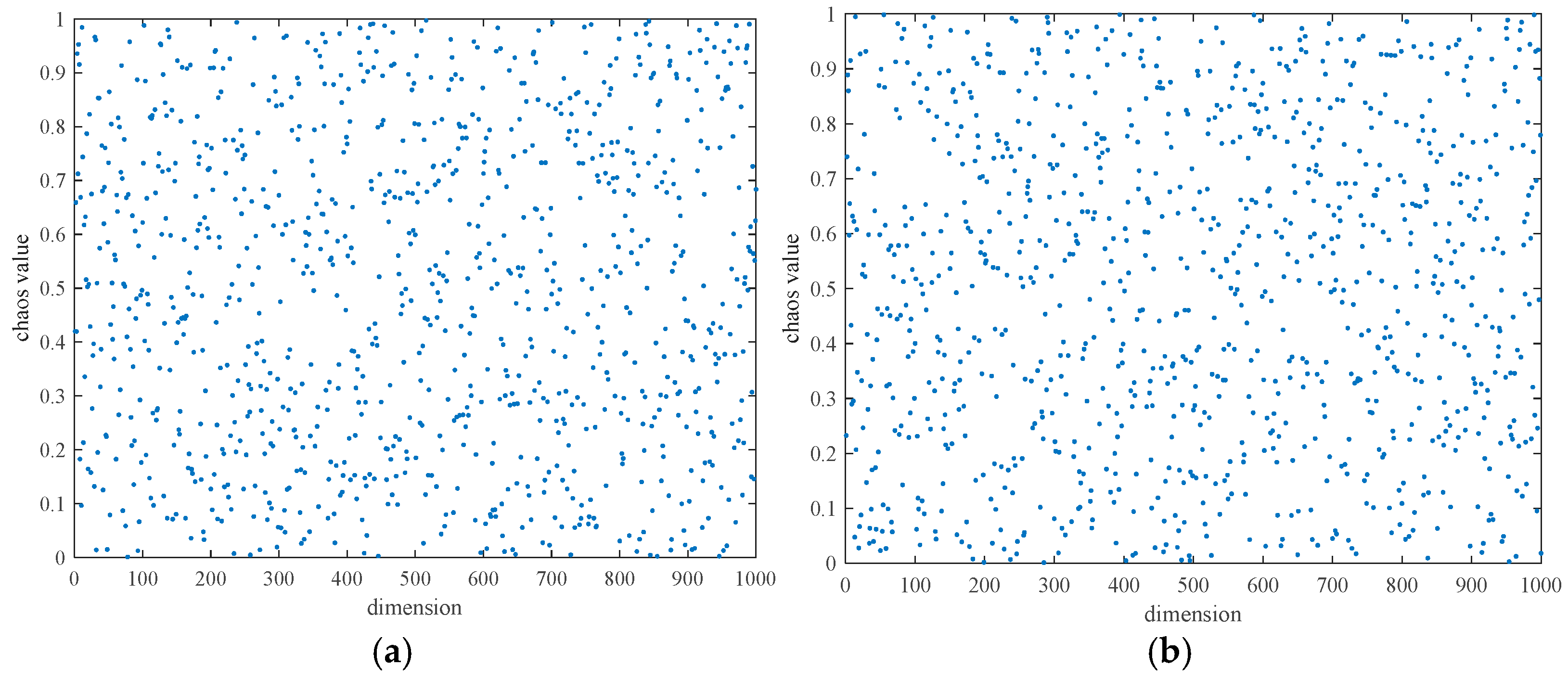
3.1. Population Initialization Based on Logistic Mapping
3.2. Improved Black-Winged Kite Algorithm with Fusion of Osprey
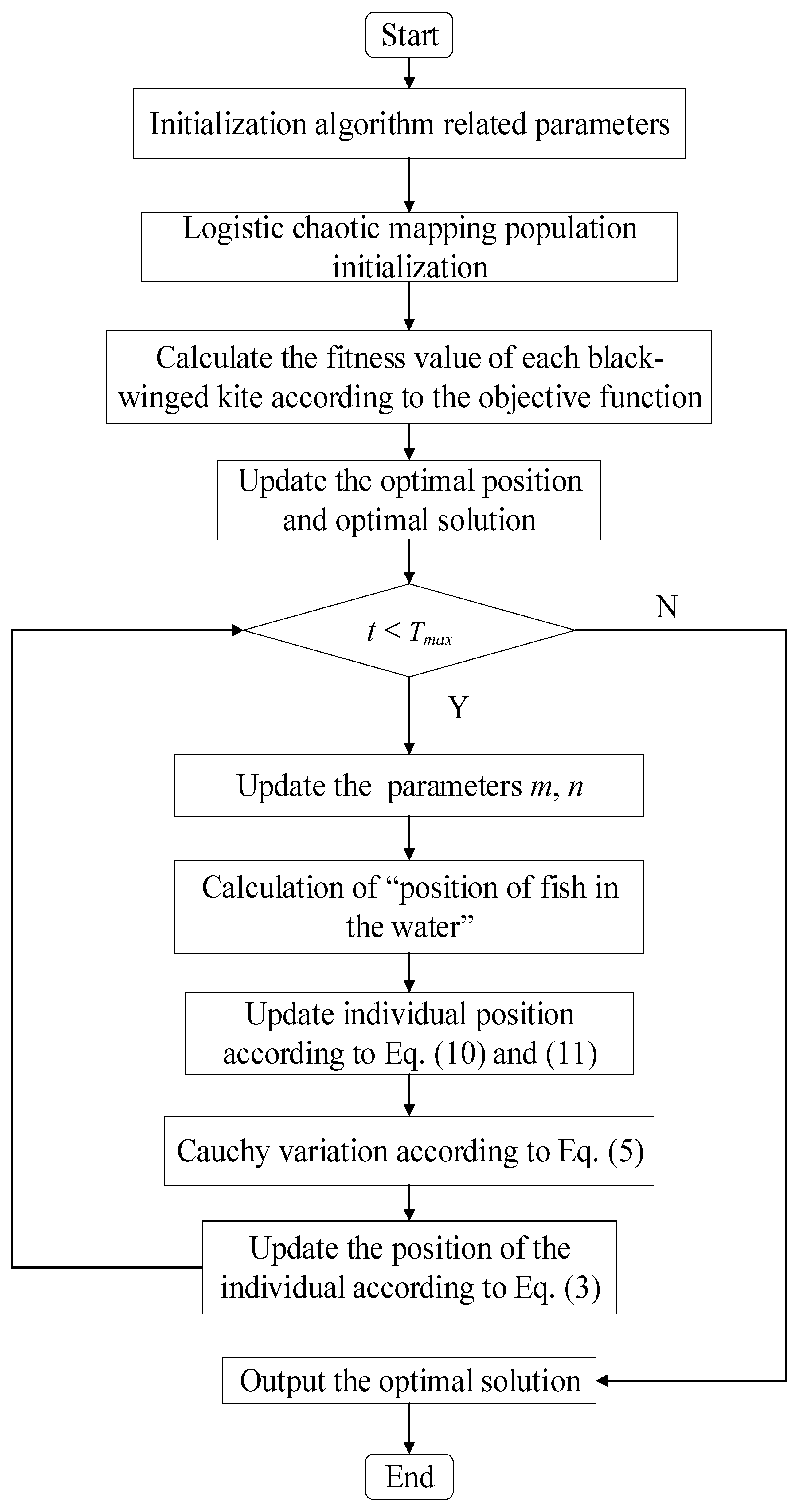
3.3. The OCBKA Flowchart and Pseudocode
| Algorithm 1. Pseudocode of OCBKA |
| Inputs: the maximum number of iterations is T, the size of the population is N. Output: optimal position, Xbest, and fitness value, F(Xbest). |
|
3.4. Time Complexity Analysis
4. Experimental Comparison and Result Analysis
4.1. Experimental Setup
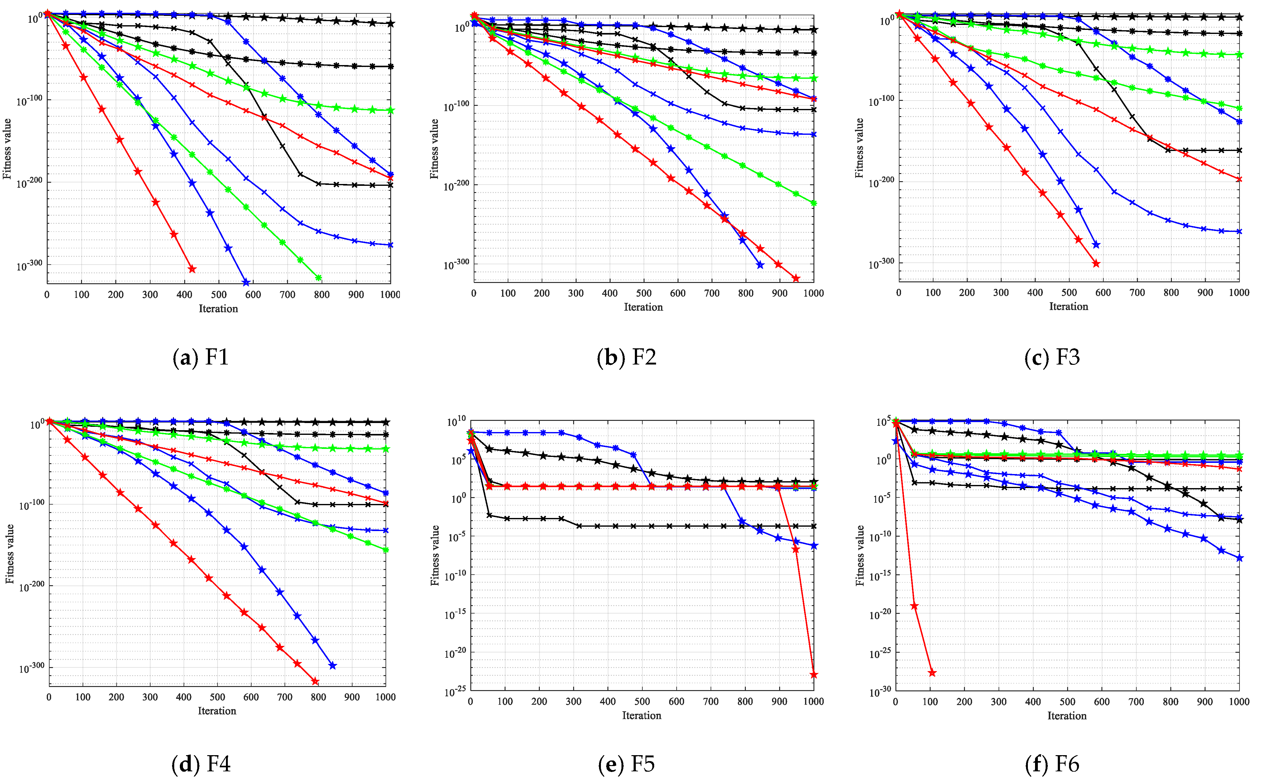
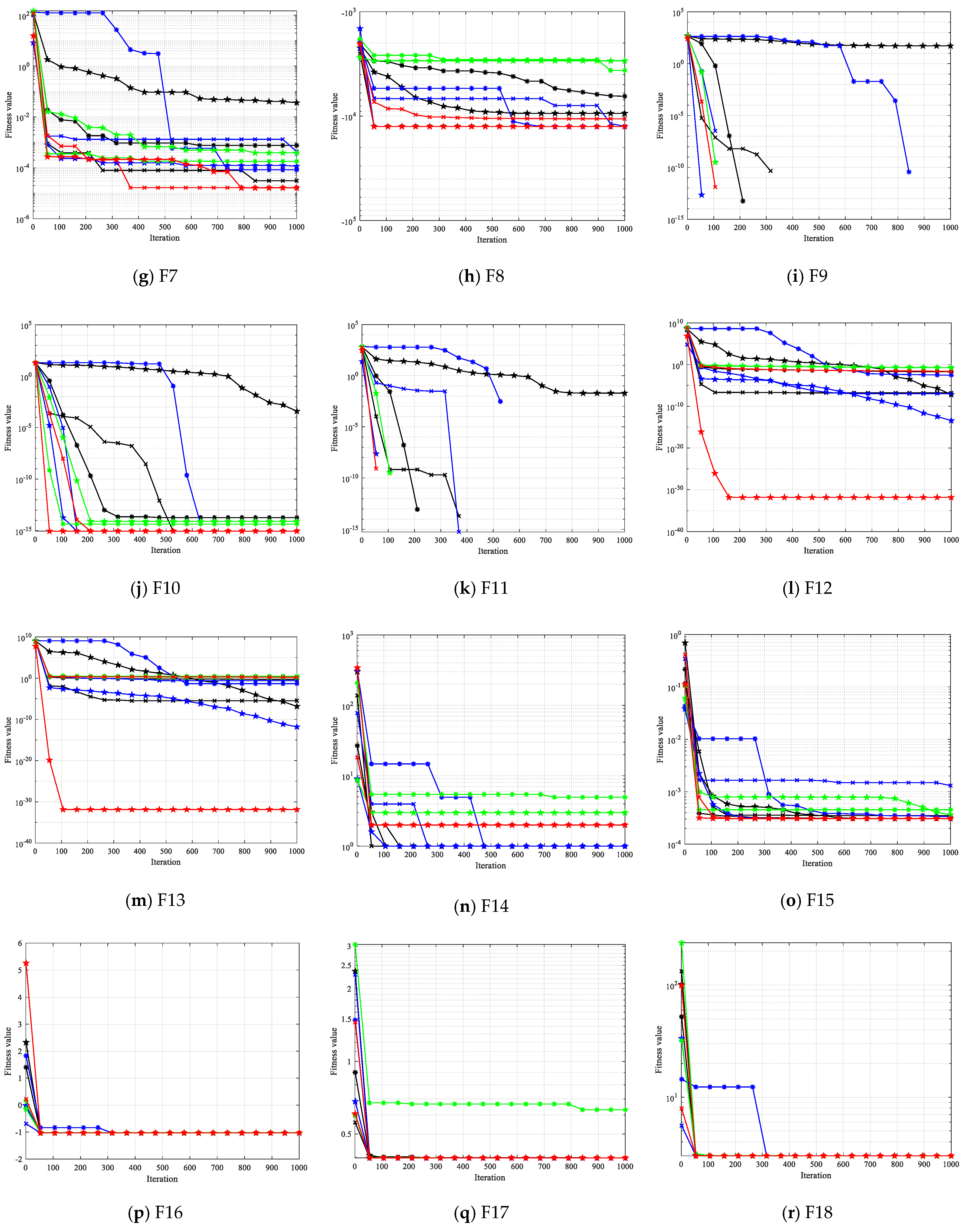
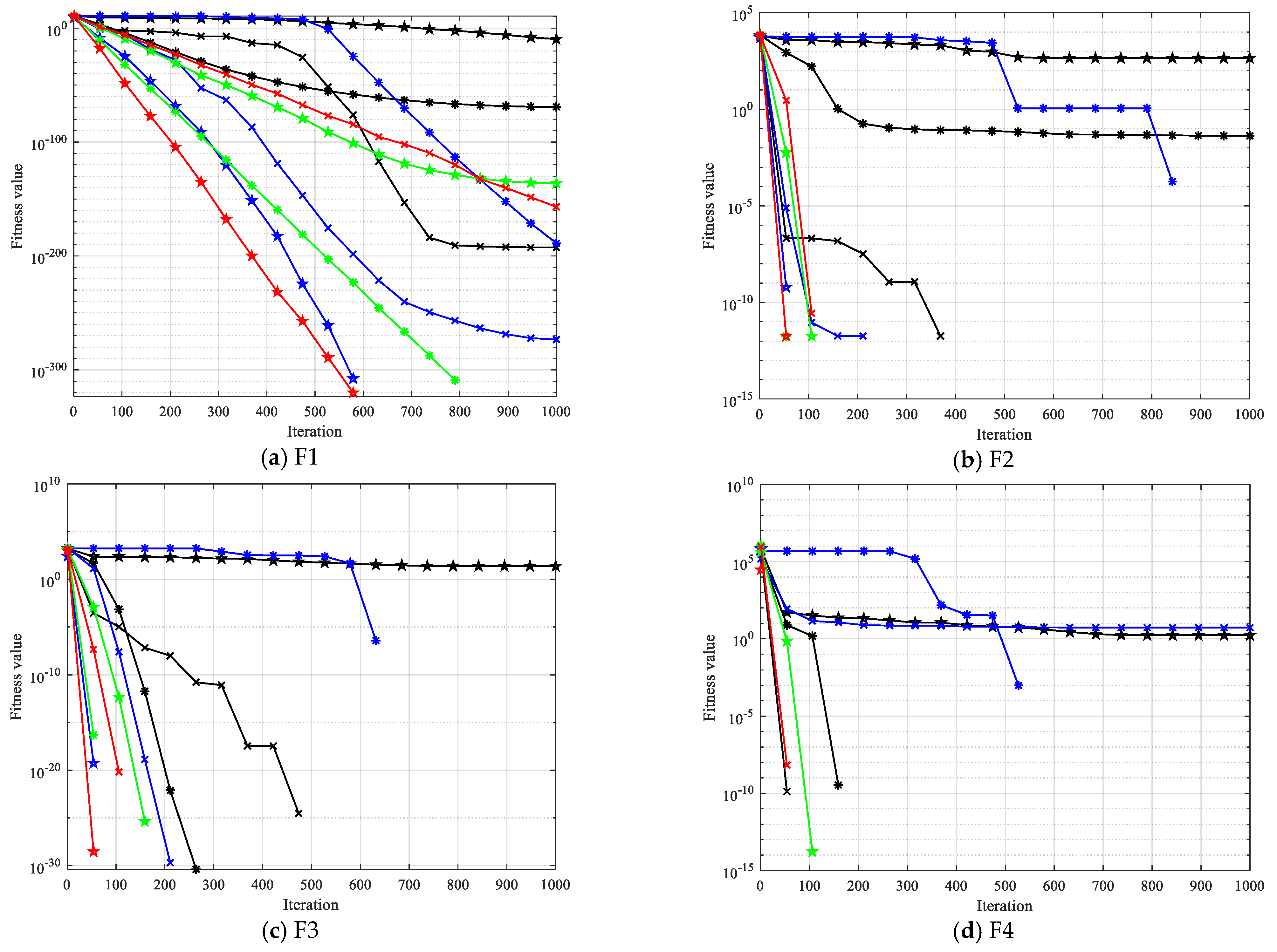
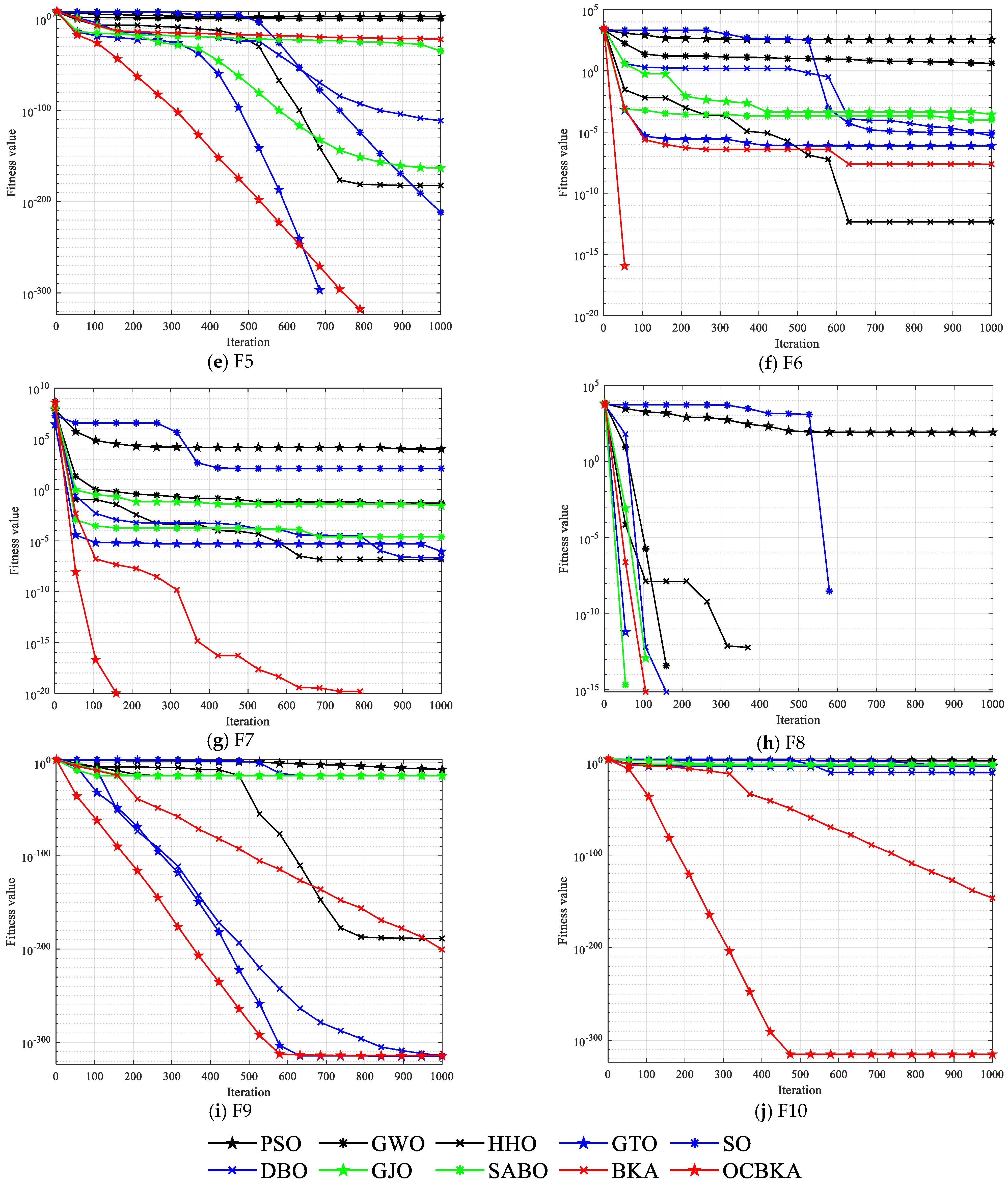
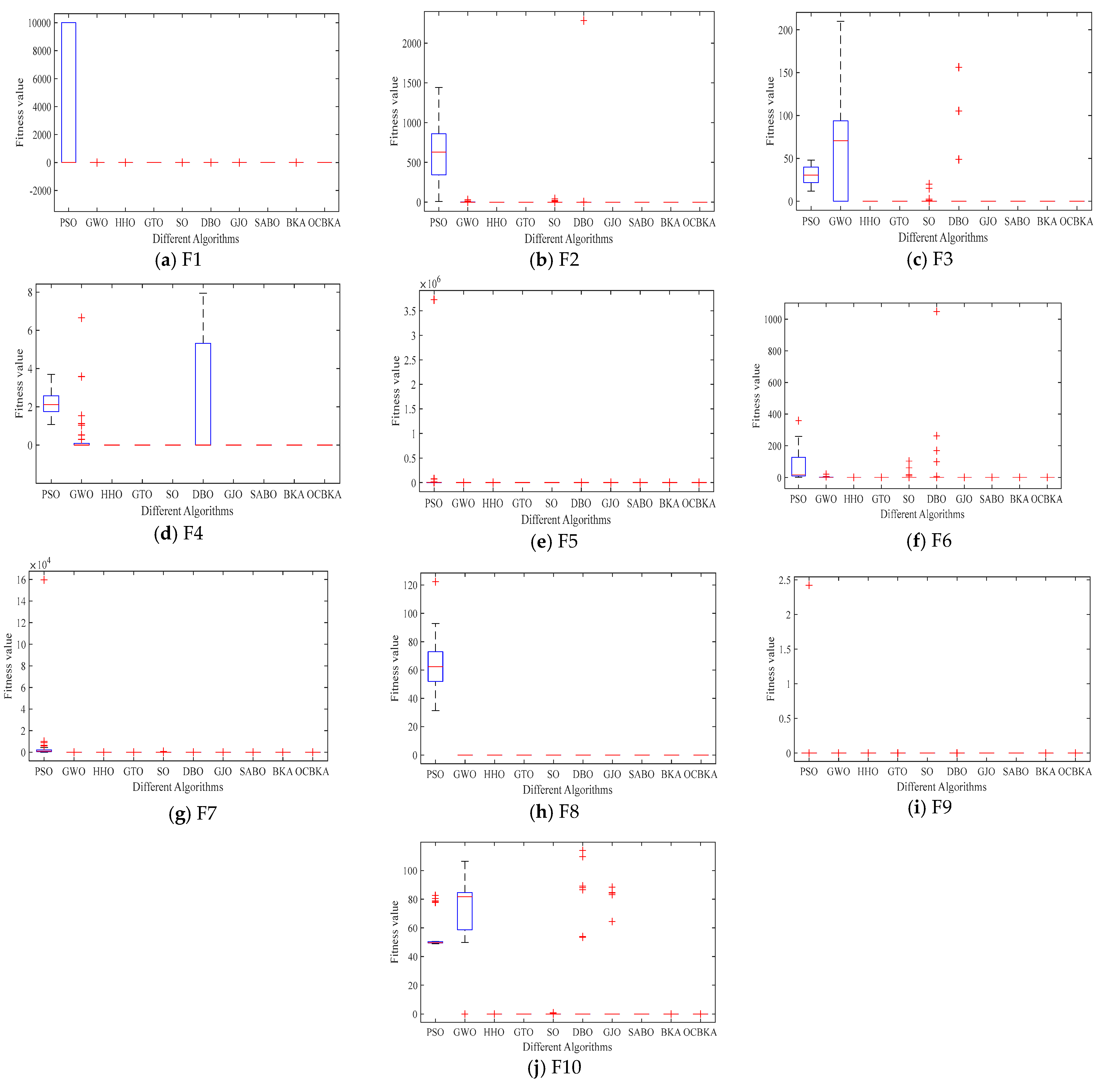
4.2. Comparative Experiment with Classical Swarm Intelligence Algorithm
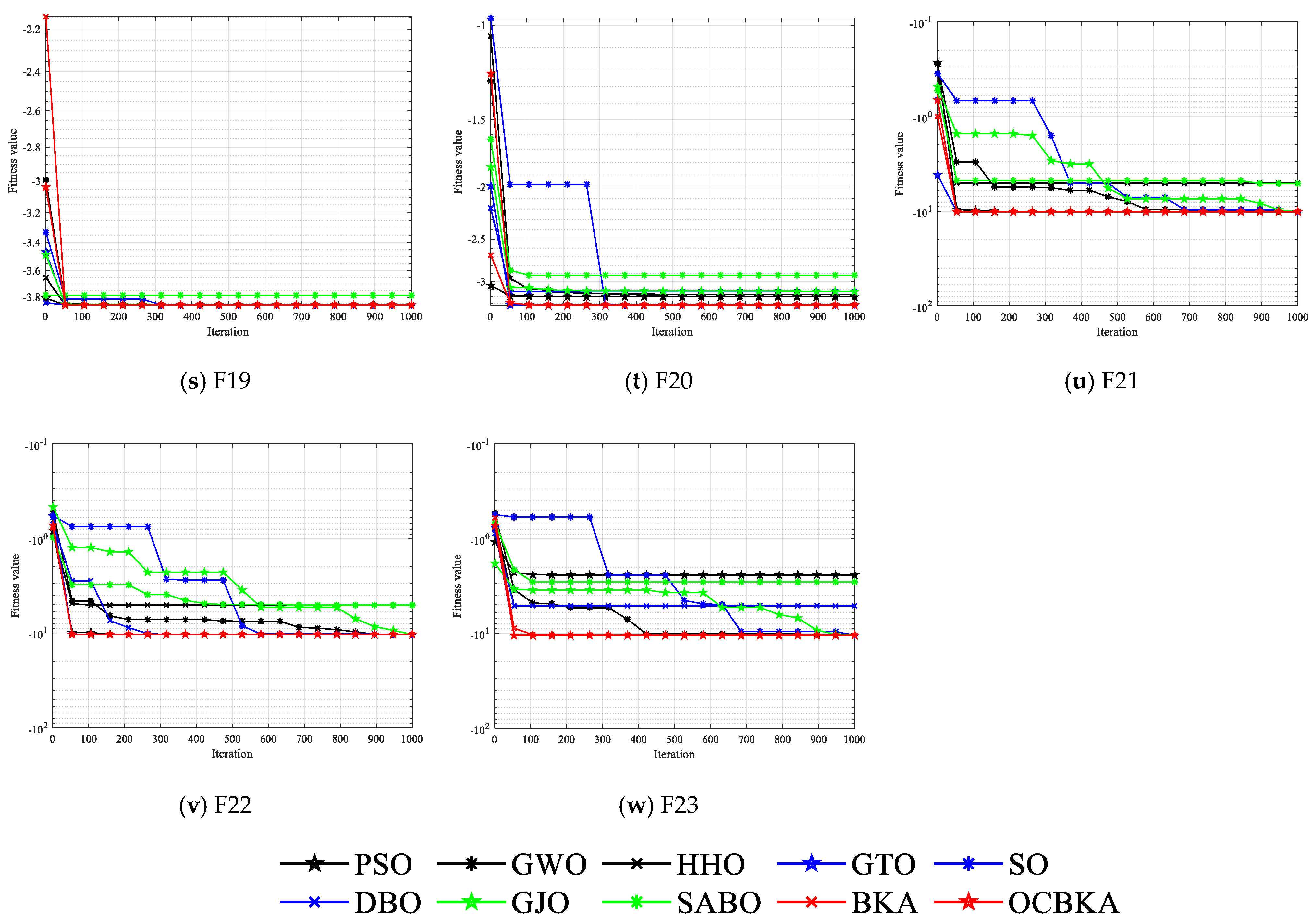
4.3. Further Comparative Experiments of Algorithms
4.4. Application of OCBKA in Engineering Optimization Problems
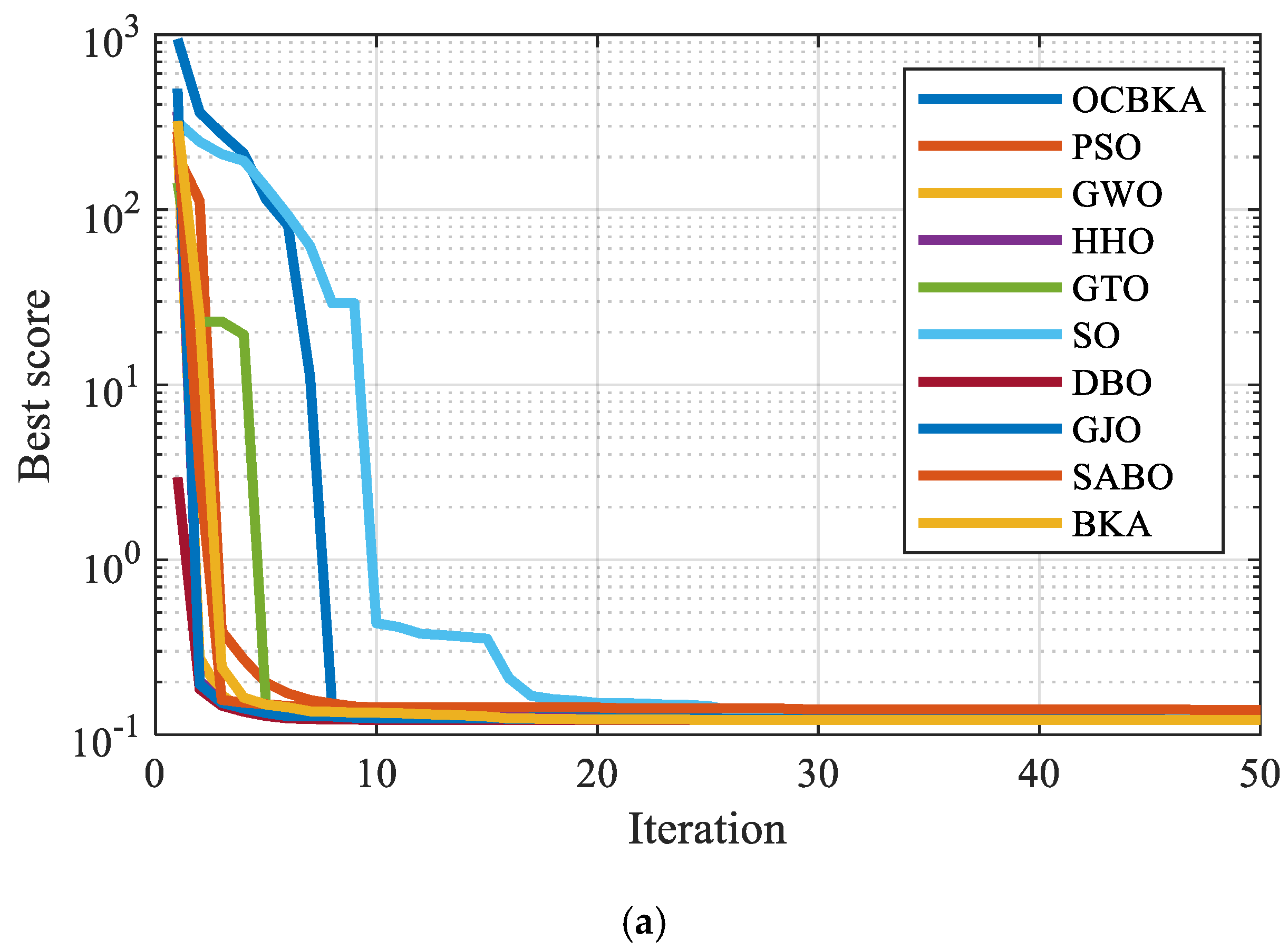
4.4.1. Tension/Compression Spring Design Optimization Problem
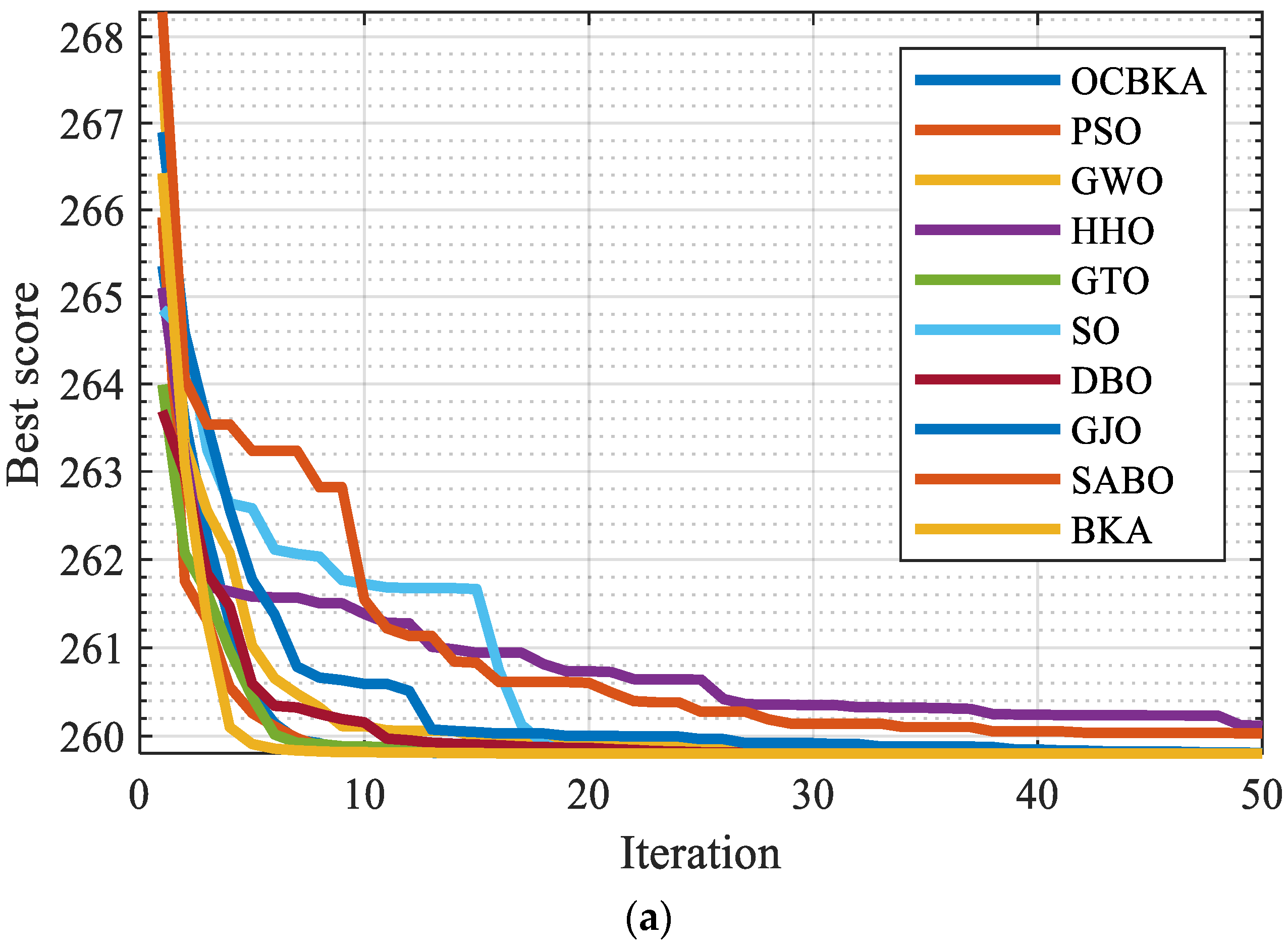
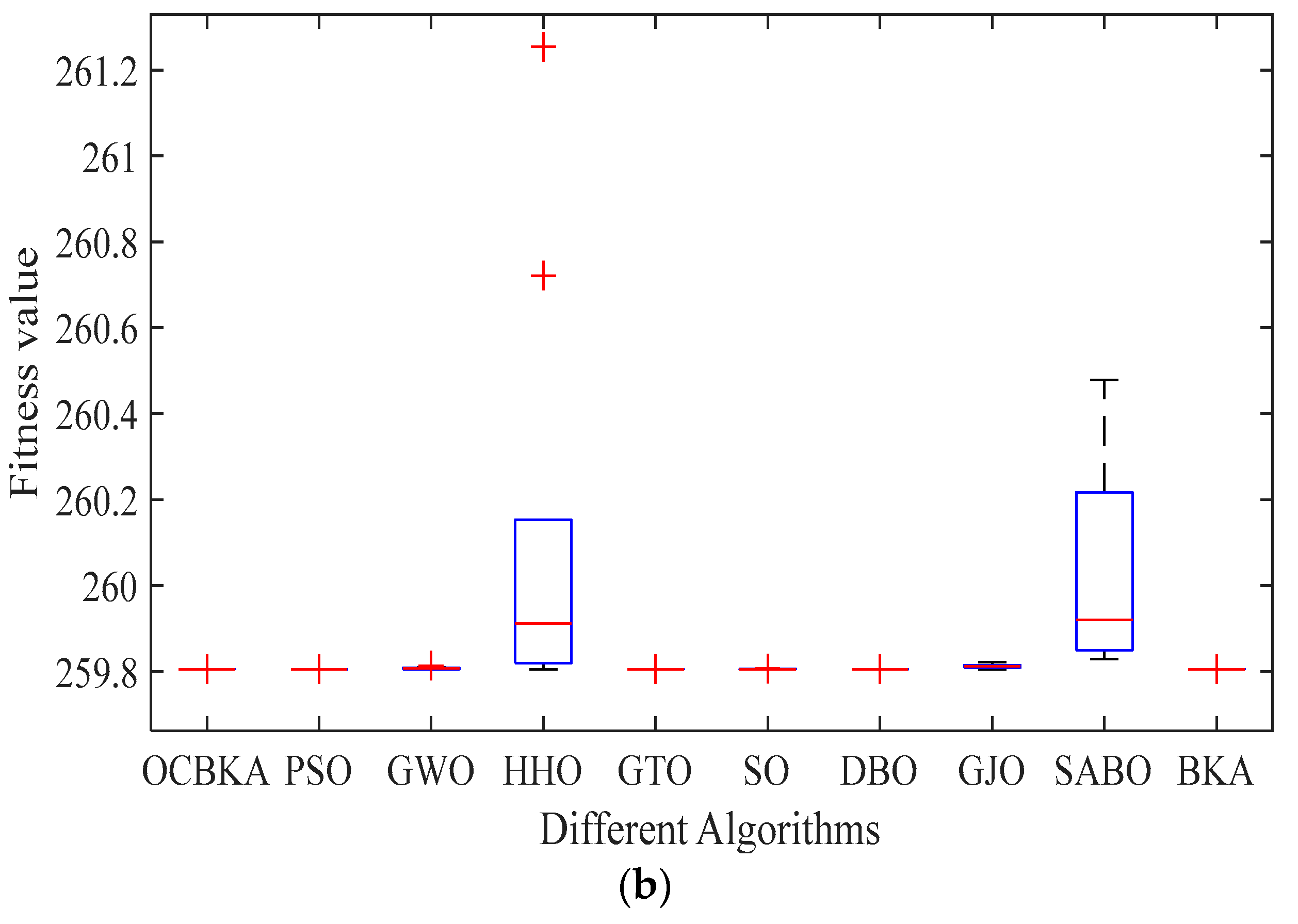
4.4.2. Three-Bar Truss Design Problem
4.4.3. Weight Minimization of a Speed Reducer
5. Conclusions
Author Contributions
Funding
Institutional Review Board Statement
Data Availability Statement
Conflicts of Interest
References
- Kivi, M.E.; Majidnezhad, V. A novel swarm intelligence algorithm inspired by the grazing of sheep. J. Ambient. Intell. Humaniz. Comput. 2022, 13, 1201–1213. [Google Scholar] [CrossRef]
- Madani, A.; Engelbrecht, A.; Ombuki-Berman, B. Cooperative coevolutionary multi-guide particle swarm optimization algorithm for large-scale multi-objective optimization problems. Swarm Evol. Comput. 2023, 78, 101262. [Google Scholar] [CrossRef]
- Tang, J.; Duan, H.; Lao, S. Swarm intelligence algorithms for multiple unmanned aerial vehicles collaboration: A comprehensive review. Artif. Intell. Rev. 2023, 56, 4295–4327. [Google Scholar] [CrossRef]
- Chen, C.; Cao, L.; Chen, Y.; Chen, B.; Yue, Y. A comprehensive survey of convergence analysis of beetle antennae search algorithm and its applications. Artif. Intell. Rev. 2024, 57, 141. [Google Scholar] [CrossRef]
- Cao, L.; Chen, H.; Chen, Y.; Yinggao Yue Zhang, X. Bio-Inspired Swarm Intelligence Optimization Algorithm-Aided Hybrid TDOA/AOA-Based Localization. Biomimetics 2023, 8, 186. [Google Scholar] [CrossRef]
- Yue, Y.; Cao, L.; Chen, H.; Chen, Y.; Su, Z. Towards an Optimal KELM Using the PSO-BOA Optimization Strategy with Applications in Data Classification. Biomimetics 2023, 8, 306. [Google Scholar] [CrossRef]
- Chen, B.; Cao, L.; Chen, C.; Chen, Y.; Yue, Y. A comprehensive survey on the chicken swarm optimization algorithm and its applications: State-of-the-art and research challenges. Artif. Intell. Rev. 2024, 57, 170. [Google Scholar] [CrossRef]
- Yue, Y.; Cao, L.; Zhang, Y. Novel WSN Coverage Optimization Strategy Via Monarch Butterfly Algorithm and Particle Swarm Optimization. Wirel. Pers. Commun. 2024, 135, 2255–2280. [Google Scholar] [CrossRef]
- Hosny, K.M.; Khalid, A.M.; Said, W.; Elmezain, M.; Mirjalili, S. A novel metaheuristic based on object-oriented programming concepts for engineering optimization. Alex. Eng. J. 2024, 98, 221–248. [Google Scholar] [CrossRef]
- Wang, S.; Cao, L.; Chen, Y.; Chen, C.; Yue, Y.; Zhu, W. Gorilla optimization algorithm combining sine cosine and cauchy variations and its engineering applications. Sci. Rep. 2024, 14, 7578. [Google Scholar] [CrossRef]
- Cao, L.; Wang, Z.; Wang, Z.; Wang, X.; Yue, Y. An Energy-Saving and Efficient Deployment Strategy for Heterogeneous Wireless Sensor Networks Based on Improved Seagull Optimization Algorithm. Biomimetics 2023, 8, 231. [Google Scholar] [CrossRef] [PubMed]
- Yue, Y.; Cao, L.; Lu, D.; Hu, Z.; Xu, M.; Wang, S.; Li, B.; Ding, H. Review and empirical analysis of sparrow search algorithm. Artif. Intell. Rev. 2023, 56, 10867–10919. [Google Scholar] [CrossRef]
- Faris, H.; Aljarah, I.; Al-Betar, M.A.; Mirjalili, S. Grey wolf optimizer: A review of recent variants and applications. Neural Comput. Appl. 2018, 30, 413–435. [Google Scholar] [CrossRef]
- Yue, Y.; You, H.; Wang, S.; Cao, L. Improved whale optimization algorithm and its application in heterogeneous wireless sensor networks. Int. J. Distrib. Sens. Netw. 2021, 17, 15501477211018140. [Google Scholar] [CrossRef]
- Wang, J.; Wang, W.-C.; Hu, X.-X.; Qiu, L.; Zang, H.-F. Black-winged kite algorithm: A nature-inspired meta-heuristic for solving benchmark functions and engineering problems. Artif. Intell. Rev. 2024, 57, 98. [Google Scholar] [CrossRef]
- Thu, Q.M.; Cuong, T.M. Solving the economic load dispatch integrating clean energies in power system using Black Kite Algorithm. World J. Adv. Eng. Technol. Sci. 2024, 11, 592–600. [Google Scholar]
- Abdel-Basset, M.; Mohamed, R.; Hezam, I.M.; Sallam, K.M.; Hameed, I.A. Parameters identification of photovoltaic models using Lambert W-function and Newton-Raphson method collaborated with AI-based optimization techniques: A comparative study. Expert Syst. Appl. 2024, 255, 124777. [Google Scholar] [CrossRef]
- Zhang, S.; Lee, C.K.; Chan, H.K.; Choy, K.L.; Wu, Z. Swarm intelligence applied in green logistics: A literature review. Eng. Appl. Artif. Intell. 2015, 37, 154–169. [Google Scholar] [CrossRef]
- Xu, J.; Di Nardo, M.; Yin, S. Improved Swarm Intelligence-Based Logistics Distribution Optimizer: Decision Support for Multimodal Transportation of Cross-Border E-Commerce. Mathematics 2024, 12, 763. [Google Scholar] [CrossRef]
- Dehghani, M.; Trojovský, P. Osprey optimization algorithm: A new bio-inspired metaheuristic algorithm for solving engineering optimization problems. Front. Mech. Eng. 2023, 8, 1126450. [Google Scholar] [CrossRef]
- Ismaeel, A.A.K.; Houssein, E.H.; Khafaga, D.S.; Aldakheel, E.A.; AbdElrazek, A.S.; Said, M. Performance of osprey optimization algorithm for solving economic load dispatch problem. Mathematics 2023, 11, 4107. [Google Scholar] [CrossRef]
- Yuan, Y.; Yang, Q.; Ren, J.; Mu, X.; Wang, Z.; Shen, Q.; Zhao, W. Attack-defense strategy assisted osprey optimization algorithm for PEMFC parameters identification. Renew. Energy 2024, 225, 120211. [Google Scholar] [CrossRef]
- Zhang, Y.; Liu, P. Research on reactive power optimization based on hybrid osprey optimization algorithm. Energies 2023, 16, 7101. [Google Scholar] [CrossRef]
- Somula, R.; Cho, Y.; Mohanta, B.K. SWARAM: Osprey optimization algorithm-based energy-efficient cluster head selection for wireless sensor network-based internet of things. Sensors 2024, 24, 521. [Google Scholar] [CrossRef] [PubMed]
- Aribowo, W.; Suryoatmojo, H.; Pamuji, F.A. Improved Droop Control Based on Modified Osprey Optimization Algorithm in DC Microgrid. J. Robot. Control. 2024, 5, 804–820. [Google Scholar]
- Yasear, S.A.; Ku-Mahamud, K.R. Review of the multi-objective swarm intelligence optimization algorithms. J. Inf. Commun. Technol. 2021, 20, 171–211. [Google Scholar] [CrossRef]
- Wang, D.; Tan, D.; Liu, L. Particle swarm optimization algorithm: An overview. Soft Comput. 2018, 22, 387–408. [Google Scholar] [CrossRef]
- Nadimi-Shahraki, M.H.; Taghian, S.; Mirjalili, S. An improved grey wolf optimizer for solving engineering problems. Expert Syst. Appl. 2021, 166, 113917. [Google Scholar] [CrossRef]
- Heidari, A.A.; Mirjalili, S.; Faris, H.; Aljarah, I.; Mafarja, M.; Chen, H. Harris hawks optimization: Algorithm and applications. Future Gener. Comput. Syst. 2019, 97, 849–872. [Google Scholar] [CrossRef]
- AbAbdollahzadeh, B.; Gharehchopogh, F.S.; Mirjalili, S. Artificial gorilla troops optimizer: A new nature-inspired metaheuristic algorithm for global optimization problems. Int. J. Intell. Syst. 2021, 36, 5887–5958. [Google Scholar] [CrossRef]
- Hashim, F.A.; Hussien, A.G. Snake Optimizer: A novel meta-heuristic optimization algorithm. Knowl. Based Syst. 2022, 242, 108320. [Google Scholar] [CrossRef]
- Xue, J.; Shen, B. Dung beetle optimizer: A new meta-heuristic algorithm for global optimization. J. Supercomput. 2023, 79, 7305–7336. [Google Scholar] [CrossRef]
- Chopra, N.; Ansari, M.M. Golden jackal optimization: A novel nature-inspired optimizer for engineering applications. Expert Syst. Appl. 2022, 198, 116924. [Google Scholar] [CrossRef]
- Yang, T.; Sun, X.; Yang, H.; Liu, Y.; Zhao, H.; Dong, Z.; Mu, S. Integrated thermal error modeling and compensation of machine tool feed system using subtraction-average-based optimizer-based CNN-GRU neural network. Int. J. Adv. Manuf. Technol. 2024, 131, 6075–6089. [Google Scholar] [CrossRef]
- Tang, J.; Liu, G.; Pan, Q. A review on representative swarm intelligence algorithms for solving optimization problems: Applications and trends. IEEE/CAA J. Autom. Sin. 2021, 8, 1627–1643. [Google Scholar] [CrossRef]
- Tzanetos, A.; Blondin, M. A qualitative systematic review of metaheuristics applied to tension/compression spring design problem: Current situation, recommendations, and research direction. Eng. Appl. Artif. Intell. 2023, 118, 105521. [Google Scholar] [CrossRef]
- Đurðev, M.; Desnica, E.; Pekez, J.; Milošević, M.; Lukić, D.; Novaković, B.; Đorðevič, L. Modern swarm-based algorithms for the tension/compression spring design optimization problem. Ann. Fac. Eng. Hunedoara 2021, 19, 55–58. [Google Scholar]
- Hussien, A.G. An enhanced opposition-based salp swarm algorithm for global optimization and engineering problems. J. Ambient. Intell. Humaniz. Comput. 2022, 13, 129–150. [Google Scholar] [CrossRef]
- Seyyedabbasi, A.; Kiani, F. Sand Cat swarm optimization: A nature-inspired algorithm to solve global optimization problems. Eng. Comput. 2023, 39, 2627–2651. [Google Scholar] [CrossRef]
- Fauzi, H.; Batool, U. A three-bar truss design using single-solution simulated Kalman filter optimizer. Mekatronika J. Intell. Manuf. Mechatron. 2019, 1, 98–102. [Google Scholar] [CrossRef]
- Kumar, A. Application of nature-inspired computing paradigms in optimal design of structural engineering problems—A review. Nat. Inspired Comput. Paradig. Syst. 2021, 63–74. [Google Scholar] [CrossRef]
- Che, Y.; He, D. An enhanced seagull optimization algorithm for solving engineering optimization problems. Appl. Intell. 2022, 52, 13043–13081. [Google Scholar] [CrossRef]
- Bhadoria, A.; Marwaha, S.; Kamboj, V.K. A solution to statistical and multidisciplinary design optimization problems using hGWO-SA algorithm. Neural Comput. Appl. 2021, 33, 3799–3824. [Google Scholar] [CrossRef]
- Tilahun, S.L.; Matadi, M.B. Weight minimization of a speed reducer using prey predator algorithm. Int. J. Manuf. Mater. Mech. Eng. 2018, 8, 19–32. [Google Scholar] [CrossRef]


| Number | Function | Theoretical Value | |
|---|---|---|---|
| F1 | Sphere Function | 0 | |
| F2 | Schwefel’s Problem 2.22 | 0 | |
| Unimodal | F3 | Schwefel’s Problem 1.2 | 0 |
| Functions | F4 | Schwefel’s Problem 2.21 | 0 |
| F5 | Generalized Rosenbrock’s Function | 0 | |
| F6 | Step Function | 0 | |
| F7 | Quartic Function, i.e., Noise | 0 | |
| F8 | Generalized Schwefel’s Problem 2.26 | −12,569.5 | |
| Simple | F9 | Generalized Rastrigin’s Function | 0 |
| Multimodal | F10 | Ackley’s Function | 0 |
| Functions | F11 | Generalized Griewank’s Function | 0 |
| F12 | Generalized Penalized Function 1 | 0 | |
| F13 | Generalized Penalized Function 2 | 0 | |
| F14 | Shekel’s Foxholes Function | 0.99800383 | |
| F15 | Kowalik’s Function | 0.0003075 | |
| F16 | Six-Hump Camel-Back Function | −1.03162845 | |
| F17 | Branin Function | 0.39788735 | |
| Composition | F18 | Goldstein–Price Function | 2.99999999 |
| Functions | F19 | Hartman’s Family | −3.86278214 |
| F20 | Hartman’s Family | −3.32199517 | |
| F21 | Shekel’s Family | −10 | |
| F22 | Shekel’s Family | −10 | |
| F23 | Shekel’s Family | −10 |
| PSO | GWO | HHO | GTO | SO | DBO | GJO | SABO | BKA | OCBKA | ||
|---|---|---|---|---|---|---|---|---|---|---|---|
| best | 1.12 × 10⁻⁹ | 2.63 × 10−61 | 5.07 × 10−212 | 0 | 3.40 × 10−192 | 0.00 × 100 | 1.07 × 10−116 | 0.00 × 100 | 1.36 × 10−205 | 0.00 × 100 | |
| std. | 1.78 × 10⁻⁶ | 8.96 × 10−59 | 0 | 0 | 0 | 0 | 9.67 × 10−110 | 0.00 × 100 | 8.06 × 10−144 | 0.00 × 100 | |
| F1 | avg. | 6.02 × 10⁻⁷ | 4.32 × 10−59 | 1.41 × 10−185 | 0.00 × 100 | 1.72 × 10−186 | 8.81 × 10−248 | 1.78 × 10−110 | 0.00 × 100 | 1.47 × 10−144 | 0.00 × 100 |
| time | 6.64 × 10⁻² | 1.19 × 10⁻¹ | 1.05 × 10⁻¹ | 2.42 × 10⁻¹ | 6.67 × 10⁻² | 1.10 × 10⁻¹ | 1.60 × 10⁻¹ | 1.42 × 10⁻¹ | 1.06 × 10⁻¹ | 1.97 × 10⁻¹ | |
| convergence | Yes | Yes | Yes | Yes | Yes | Yes | Yes | Yes | Yes | Yes | |
| best | 6.61 × 10⁻⁶ | 9.41 × 10−36 | 1.66 × 10−108 | 0.00 × 100 | 5.54 × 10−98 | 3.37 × 10−166 | 8.42 × 10−69 | 2.54 × 10−227 | 1.42 × 10−105 | 0.00 × 100 | |
| std. | 3.45 × 100 | 1.18 × 10⁻³⁴ | 1.10 × 10−95 | 0.00 × 100 | 1.86 × 10−90 | 6.24 × 10−120 | 4.68 × 10−66 | 0.00 × 100 | 2.85 × 10−84 | 0.00 × 100 | |
| F2 | avg. | 1.33 × 100 | 1.19 × 10⁻³⁴ | 2.03 × 10−96 | 0.00 × 100 | 6.89 × 10−91 | 1.14 × 10−120 | 2.99 × 10−66 | 6.06 × 10−223 | 6.34 × 10−85 | 0.00 × 100 |
| time | 6.27 × 10⁻² | 1.22 × 10⁻¹ | 9.90 × 10⁻² | 2.41 × 10⁻¹ | 5.62 × 10⁻² | 1.05 × 10⁻¹ | 1.56 × 10⁻¹ | 1.41 × 10⁻¹ | 9.60 × 10⁻² | 2.18 × 10⁻¹ | |
| convergence | Yes | Yes | Yes | Yes | Yes | Yes | Yes | Yes | Yes | Yes | |
| best | 146.96 × 100 | 2.39 × 10⁻¹⁹ | 3.73 × 10−179 | 0.00 × 100 | 9.82 × 10−140 | 3.49 × 10−276 | 8.43 × 10−48 | 5.68 × 10−176 | 3.74 × 10−204 | 0.00 × 100 | |
| std. | 3.24 × 10³ | 1.69 × 10⁻¹⁴ | 1.76 × 10−143 | 0.00 × 100 | 4.52 × 10−122 | 3.84 × 10−158 | 1.03 × 10−37 | 4.90 × 10−81 | 0.00 × 100 | 0.00 × 100 | |
| F3 | avg. | 2.06 × 10³ | 5.72 × 10⁻¹⁵ | 3.98 × 10−144 | 0.00 × 100 | 9.30 × 10−123 | 7.02 × 10−159 | 1.92 × 10−38 | 8.95 × 10−82 | 3.76 × 10−179 | 0.00 × 100 |
| time | 2.19 × 10⁻¹ | 2.79 × 10⁻¹ | 5.00 × 10⁻¹ | 5.58 × 10⁻¹ | 2.13 × 10⁻¹ | 2.64 × 10⁻¹ | 3.37 × 10⁻¹ | 3.03 × 10⁻¹ | 4.28 × 10⁻¹ | 5.52 × 10⁻¹ | |
| convergence | No | Yes | Yes | Yes | Yes | Yes | Yes | Yes | Yes | Yes | |
| best | 1.98 × 100 | 6.31 × 10⁻¹⁶ | 1.70 × 10−105 | 0.00 × 100 | 1.29 × 10−89 | 1.93 × 10−157 | 1.94 × 10−36 | 4.73 × 10−158 | 1.6 × 10−103 | 0.00 × 100 | |
| std. | 1.01 × 100 | 1.17 × 10⁻¹⁴ | 1.12 × 10−91 | 0.00 × 100 | 6.55 × 10−85 | 7.05 × 10−113 | 4.12 × 10⁻³³ | 8.51 × 10−155 | 2.12 × 10−75 | 0.00 × 100 | |
| F4 | avg. | 3.97 × 100 | 1.11 × 10⁻¹⁴ | 2.93 × 10−92 | 0.00 × 100 | 3.52 × 10−85 | 1.29 × 10−113 | 1.91 × 10⁻³³ | 4.20 × 10−155 | 3.87 × 10−76 | 0.00 × 100 |
| time | 6.13 × 10⁻² | 1.21 × 10⁻¹ | 1.28 × 10⁻¹ | 2.36 × 10⁻¹ | 5.00 × 10⁻² | 9.81 × 10⁻² | 1.53 × 10⁻¹ | 1.42 × 10⁻¹ | 1.04 × 10⁻¹ | 1.97 × 10⁻¹ | |
| convergence | No | Yes | Yes | Yes | Yes | Yes | Yes | Yes | Yes | Yes | |
| best | 2.28 × 101 | 2.57 × 101 | 1.02 × 10⁻⁵ | 8.4 × 10⁻⁸ | 1.82 × 10⁻¹ | 2.45 × 101 | 2.59 × 101 | 2.70 × 101 | 2.49 × 101 | 0.00 × 100 | |
| std. | 1.64 × 10⁴ | 7.33 × 10⁻¹ | 3.08 × 10⁻³ | 3.97 × 100 | 1.25 × 101 | 1.73 × 10⁻¹ | 9.54 × 10⁻¹ | 6.12 × 10⁻¹ | 1.22 × 100 | 1.31 × 101 | |
| F5 | avg. | 3.39 × 10³ | 2.70 × 101 | 0.26 × 10⁻³ | 7.26 × 10⁻¹ | 1.39 × 101 | 2.49 × 101 | 2.76 × 101 | 2.80 × 101 | 2.71 × 101 | 1.38 × 101 |
| time | 8.23 × 10⁻² | 1.35 × 10⁻¹ | 1.99 × 10⁻¹ | 2.56 × 10⁻¹ | 7.03 × 10⁻² | 1.20 × 10⁻¹ | 1.74 × 10⁻¹ | 1.57 × 10⁻¹ | 1.43 × 10⁻¹ | 2.40 × 10⁻¹ | |
| convergence | No | Yes | Yes | Yes | Yes | No | Yes | Yes | Yes | Yes | |
| best | 6.34 × 10⁻¹⁰ | 2.1 × 10⁻⁵ | 4.77 × 10⁻⁸ | 4.61 × 10⁻¹⁶ | 9.27 × 10⁻⁷ | 7.24 × 10⁻¹¹ | 1.75 × 100 | 1.22 × 100 | 7.26 × 10⁻⁵ | 0.00 × 100 | |
| std. | 1.72 × 10⁻⁵ | 4.17 × 10⁻¹ | 4.30 × 10⁻⁵ | 8.08 × 10⁻¹² | 2.73 × 100 | 2.01 × 10⁻⁷ | 3.77 × 10⁻¹ | 6.01 × 10⁻¹ | 1.58 × 100 | 1.24 × 10⁻¹² | |
| F6 | avg. | 3.27 × 10⁻⁶ | 7.35 × 10⁻¹ | 2.63 × 10⁻⁵ | 3.83 × 10⁻¹² | 2.05 × 100 | 5.75 × 10⁻⁸ | 2.59 × 100 | 2.04 × 100 | 9.91 × 10⁻¹ | 2.29 × 10⁻¹³ |
| time | 5.96 × 10⁻² | 1.17 × 10⁻¹ | 1.46 × 10⁻¹ | 2.26 × 10⁻¹ | 5.18 × 10⁻² | 9.88 × 10⁻² | 1.52 × 10⁻¹ | 1.38 × 10⁻¹ | 1.04 × 10⁻¹ | 1.91 × 10⁻¹ | |
| convergence | Yes | Yes | Yes | Yes | Yes | Yes | Yes | Yes | Yes | Yes | |
| best | 1.27 × 10⁻² | 2.66 × 10⁻⁴ | 2.32 × 10⁻⁶ | 7.9 × 10⁻⁷ | 9.6 × 10⁻⁷ | 3.56 × 10⁻⁵ | 3.41 × 10⁻⁵ | 3.25 × 10⁻⁶ | 6.60 × 10⁻⁶ | 2.97 × 10⁻⁶ | |
| std. | 1.00 × 10⁻² | 3.98 × 10⁻⁴ | 9.28 × 10⁻⁵ | 4.45 × 10⁻⁵ | 7.96 × 10⁻⁵ | 5.14 × 10⁻⁴ | 2.57 × 10⁻⁴ | 4.78 × 10⁻⁵ | 7.12 × 10⁻⁵ | 3.61 × 10⁻⁵ | |
| F7 | avg. | 2.76 × 10⁻² | 7.72 × 10⁻⁴ | 9.67 × 10⁻⁵ | 4.92 × 10⁻⁵ | 9.3 × 10⁻⁵ | 5.65 × 10⁻⁴ | 2.44 × 10⁻⁴ | 5.42 × 10⁻⁵ | 1.18 × 10⁻⁴ | 4.58 × 10⁻⁵ |
| time | 1.66 × 10⁻¹ | 2.21 × 10⁻¹ | 3.61 × 10⁻¹ | 4.30 × 10⁻¹ | 1.56 × 10⁻¹ | 2.03 × 10⁻¹ | 2.65 × 10⁻¹ | 2.42 × 10⁻¹ | 3.14 × 10⁻¹ | 4.14 × 10⁻¹ | |
| convergence | Yes | Yes | Yes | Yes | Yes | Yes | Yes | Yes | Yes | Yes | |
| best | −9.78 × 10³ | −7.15 × 10³ | −1.26 × 10⁴ | −1.26 × 10⁴ | −1.26 × 10⁴ | −1.25 × 10⁴ | −6.50 × 10³ | −4.59 × 10³ | −1.13 × 10⁴ | −1.26 × 10⁴ | |
| std. | 5.70 × 10² | 7.67 × 10² | 1.19 × 10² | 2.29 × 10⁻⁹ | 4.51 × 101 | 1.81 × 10³ | 1.03 × 10³ | 5.36 × 10² | 1.89 × 10³ | 4.75 × 101 | |
| F8 | avg. | −8.78 × 10³ | −6.04 × 10³ | −1.25 × 10⁴ | −1.26 × 10⁴ | −1.25 × 10⁴ | −8.93 × 10³ | −3.82 × 10³ | −3.20 × 10³ | −8.85 × 10³ | −1.26 × 10⁴ |
| time | 8.52 × 10⁻² | 1.43 × 10⁻¹ | 2.09 × 10⁻¹ | 2.77 × 10⁻¹ | 7.30 × 10⁻² | 1.37 × 10⁻¹ | 1.81 × 10⁻¹ | 1.62 × 10⁻¹ | 1.49 × 10⁻¹ | 2.44 × 10⁻¹ | |
| convergence | Yes | No | Yes | Yes | Yes | No | No | Yes | No | No | |
| best | 2.98 × 101 | 0.00 × 100 | 0.00 × 100 | 0.00 × 100 | 0.00 × 100 | 0.00 × 100 | 0.00 × 100 | 0.00 × 100 | 0.00 × 100 | 0.00 × 100 | |
| std. | 1.72 × 101 | 1.00 × 100 | 0.00 × 100 | 0.00 × 100 | 5.49 × 100 | 2.91 × 100 | 0.00 × 100 | 0.00 × 100 | 0.00 × 100 | 0.00 × 100 | |
| F9 | avg. | 5.82 × 101 | 3.28 × 10⁻¹ | 0.00 × 100 | 0.00 × 100 | 1.00 × 100 | 5.31 × 10⁻¹ | 0.00 × 100 | 0.00 × 100 | 0.00 × 100 | 0.00 × 100 |
| time | 7.81 × 10⁻² | 1.19 × 10⁻¹ | 1.69 × 10⁻¹ | 2.39 × 10⁻¹ | 6.56 × 10⁻² | 1.05 × 10⁻¹ | 1.59 × 10⁻¹ | 1.41 × 10⁻¹ | 1.13 × 10⁻¹ | 1.96 × 10⁻¹ | |
| convergence | Yes | Yes | Yes | Yes | Yes | Yes | Yes | Yes | Yes | Yes | |
| best | 7.31 × 10⁻⁶ | 1.51 × 10⁻¹⁴ | 8.88 × 10⁻¹⁶ | 8.88 × 10⁻¹⁶ | 8.88 × 10⁻¹⁶ | 8.88 × 10⁻¹⁶ | 4.44 × 10⁻¹⁵ | 4.44 × 10⁻¹⁵ | 8.88 × 10⁻¹⁶ | 8.88 × 10⁻¹⁶ | |
| std. | 5.36 × 10⁻¹ | 2.75 × 10⁻¹⁵ | 0.00 × 100 | 0.00 × 100 | 6.49 × 10⁻¹⁶ | 0.00 × 100 | 9.01 × 10⁻¹⁶ | 6.49 × 10⁻¹⁶ | 0.00 × 100 | 0.00 × 100 | |
| F10 | avg. | 2.55 × 10⁻¹ | 1.66 × 10⁻¹⁴ | 8.88 × 10⁻¹⁶ | 8.88 × 10⁻¹⁶ | 4.32 × 10⁻¹⁵ | 8.88 × 10⁻¹⁶ | 4.68 × 10⁻¹⁵ | 4.56 × 10⁻¹⁵ | 8.88 × 10⁻¹⁶ | 8.88 × 10⁻¹⁶ |
| time | 8.20 × 10⁻² | 1.22 × 10⁻¹ | 1.78 × 10⁻¹ | 2.37 × 10⁻¹ | 6.44 × 10⁻² | 1.08 × 10⁻¹ | 1.60 × 10⁻¹ | 1.45 × 10⁻¹ | 9.94 × 10⁻² | 2.00 × 10⁻¹ | |
| convergence | Yes | Yes | Yes | Yes | Yes | Yes | Yes | Yes | Yes | Yes | |
| best | 1.83 × 10⁻⁸ | 0.00 × 100 | 0.00 × 100 | 0.00 × 100 | 0.00 × 100 | 0.00 × 100 | 0.00 × 100 | 0.00 × 100 | 0.00 × 100 | 0.00 × 100 | |
| std. | 1.83 × 10⁻⁸ | 0.00 × 100 | 0.00 × 100 | 0.00 × 100 | 0.00 × 100 | 0.00 × 100 | 0.00 × 100 | 0.00 × 100 | 0.00 × 100 | 0.00 × 100 | |
| F11 | avg. | 1.72 × 10⁻² | 5.34 × 10⁻³ | 0.00 × 100 | 0.00 × 100 | 0.00 × 100 | 0.00 × 100 | 0.00 × 100 | 0.00 × 100 | 0.00 × 100 | 0.00 × 100 |
| time | 9.27 × 10⁻² | 1.40 × 10⁻¹ | 2.08 × 10⁻¹ | 2.62 × 10⁻¹ | 7.47 × 10⁻² | 1.25 × 10⁻¹ | 1.76 × 10⁻¹ | 1.66 × 10⁻¹ | 1.50 × 10⁻¹ | 2.30 × 10⁻¹ | |
| convergence | Yes | Yes | Yes | Yes | Yes | Yes | Yes | Yes | Yes | Yes | |
| best | 4.32 × 10⁻¹¹ | 1.31 × 10⁻² | 1.05 × 10⁻⁹ | 1.43 × 10⁻¹⁴ | 1.82 × 10⁻⁶ | 6.68 × 10⁻¹³ | 1.70 × 10⁻¹ | 5.64 × 10⁻² | 8.90 × 10⁻⁶ | 1.57 × 10⁻³² | |
| std. | 1.58 × 10⁻¹ | 1.95 × 10⁻² | 2.72 × 10⁻⁶ | 1.78 × 10⁻¹² | 8.88 × 10⁻³ | 8.54 × 10⁻⁴ | 4.97 × 10⁻² | 1.44 × 10⁻¹ | 6.96 × 10⁻² | 9.92 × 10⁻³⁴ | |
| F12 | avg. | 8.31 × 10⁻² | 3.97 × 10⁻² | 2.38 × 10⁻⁶ | 7.81 × 10⁻¹³ | 8.97 × 10⁻³ | 1.56 × 10⁻⁴ | 2.19 × 10⁻¹ | 1.57 × 10⁻¹ | 3.35 × 10⁻² | 1.60 × 10⁻³² |
| time | 3.38 × 10⁻¹ | 3.86 × 10⁻¹ | 8.11 × 10⁻¹ | 7.68 × 10⁻¹ | 3.25 × 10⁻¹ | 3.79 × 10⁻¹ | 4.80 × 10⁻¹ | 4.15 × 10⁻¹ | 6.54 × 10⁻¹ | 7.38 × 10⁻¹ | |
| convergence | Yes | Yes | Yes | Yes | Yes | Yes | Yes | Yes | Yes | Yes | |
| best | 2.38 × 10⁻⁹ | 0.197789 | 4.01 × 10⁻⁸ | 2.78 × 10⁻¹⁴ | 9.24 × 10⁻⁵ | 5.87 × 10⁻⁷ | 1.156906 | 1.343081 | 0.554653 | 1.35 × 10⁻³² | |
| std. | 1.10 × 10⁻² | 2.05 × 10⁻¹ | 3.58 × 10⁻⁵ | 1.02 × 10⁻² | 5.88 × 10⁻² | 2.92 × 10⁻¹ | 2.67 × 10⁻¹ | 5.39 × 10⁻¹ | 5.56 × 10⁻¹ | 2.63 × 10⁻² | |
| F13 | avg. | 6.61 × 10⁻³ | 5.02 × 10⁻¹ | 2.21 × 10⁻⁵ | 2.56 × 10⁻³ | 6.19 × 10⁻² | 3.14 × 10⁻¹ | 1.68 × 100 | 2.67 × 100 | 1.60 × 100 | 5.84 × 10⁻³ |
| time | 3.40 × 10⁻¹ | 3.92 × 10⁻¹ | 8.09 × 10⁻¹ | 7.77 × 10⁻¹ | 3.26 × 10⁻¹ | 3.75 × 10⁻¹ | 4.77 × 10⁻¹ | 4.17 × 10⁻¹ | 6.57 × 10⁻¹ | 7.45 × 10⁻¹ | |
| convergence | Yes | Yes | Yes | Yes | Yes | Yes | Yes | Yes | Yes | Yes | |
| best | 9.98 × 10⁻¹ | 9.98 × 10⁻¹ | 9.98 × 10⁻¹ | 9.98 × 10⁻¹ | 9.98 × 10⁻¹ | 9.98 × 10⁻¹ | 9.98 × 10⁻¹ | 9.98 × 10⁻¹ | 9.98 × 10⁻¹ | 9.98 × 10⁻¹ | |
| std. | 0.00 × 100 | 4.58 × 100 | 3.03 × 10⁻¹ | 0.00 × 100 | 4.26 × 10⁻⁷ | 1.88 × 100 | 4.35 × 100 | 2.87 × 100 | 7.38 × 10⁻¹ | 1.02 × 100 | |
| F14 | avg. | 9.98 × 10⁻¹ | 6.44 × 100 | 1.10 × 100 | 9.98 × 10⁻¹ | 9.98 × 10⁻¹ | 1.62 × 100 | 6.09 × 100 | 3.11 × 100 | 1.16 × 100 | 1.63 × 100 |
| time | 5.05 × 10⁻¹ | 5.07 × 10⁻¹ | 1.30 × 100 | 1.08 × 100 | 5.10 × 10⁻¹ | 5.62 × 10⁻¹ | 5.59 × 10⁻¹ | 5.46 × 10⁻¹ | 1.03 × 100 | 1.11 × 100 | |
| convergence | Yes | Yes | Yes | Yes | Yes | Yes | Yes | Yes | Yes | Yes | |
| best | 3.07 × 10⁻⁴ | 3.07 × 10⁻⁴ | 3.08 × 10⁻⁴ | 3.07 × 10⁻⁴ | 3.08 × 10⁻⁴ | 3.07 × 10⁻⁴ | 3.07 × 10⁻⁴ | 3.18 × 10⁻⁴ | 3.07 × 10⁻⁴ | 3.07 × 10⁻⁴ | |
| std. | 6.07 × 10⁻³ | 7.58 × 10⁻³ | 1.66 × 10⁻⁴ | 2.79 × 10⁻⁴ | 3.02 × 10⁻⁴ | 3.01 × 10⁻⁴ | 3.17 × 10⁻⁴ | 3.84 × 10⁻³ | 3.78 × 10⁻⁴ | 6.51 × 10⁻⁹ | |
| F15 | avg. | 2.48 × 10⁻³ | 3.72 × 10⁻³ | 3.62 × 10⁻⁴ | 3.99 × 10⁻⁴ | 6.26 × 10⁻⁴ | 6.12 × 10⁻⁴ | 4.22 × 10⁻⁴ | 1.24 × 10⁻³ | 4.80 × 10⁻⁴ | 3.07 × 10⁻⁴ |
| time | 3.73 × 10⁻² | 4.44 × 10⁻² | 1.21 × 10⁻¹ | 1.54 × 10⁻¹ | 3.93 × 10⁻² | 9.57 × 10⁻² | 9.21 × 10⁻² | 7.88 × 10⁻² | 9.27 × 10⁻² | 1.73 × 10⁻¹ | |
| convergence | Yes | Yes | Yes | Yes | Yes | Yes | Yes | Yes | Yes | Yes | |
| best | −1.03 × 100 | −1.03 × 100 | −1.03 × 100 | −1.03 × 100 | −1.03 × 100 | −1.03 × 100 | −1.03 × 100 | −1.03 × 100 | −1.03 × 100 | −1.03 × 100 | |
| std. | 6.71 × 10⁻¹⁶ | 5.67 × 10⁻⁹ | 3.38 × 10⁻¹¹ | 6.71 × 10⁻¹⁶ | 1.49 × 10⁻¹ | 6.25 × 10⁻¹⁶ | 4.21 × 10⁻⁸ | 1.23 × 10⁻² | 6.12 × 10⁻¹⁶ | 6.25 × 10⁻¹⁶ | |
| F16 | avg. | −1.03 × 100 | −1.03 × 100 | −1.03 × 100 | −1.03 × 100 | −1.00 × 100 | −1.03 × 100 | −1.03 × 100 | −1.03 × 100 | −1.03 × 100 | −1.03 × 100 |
| time | 3.95 × 10⁻² | 4.17 × 10⁻² | 1.27 × 10⁻¹ | 1.54 × 10⁻¹ | 3.87 × 10⁻² | 9.36 × 10⁻² | 8.64 × 10⁻² | 7.58 × 10⁻² | 9.00 × 10⁻² | 1.60 × 10⁻¹ | |
| convergence | Yes | Yes | Yes | Yes | Yes | Yes | Yes | Yes | Yes | Yes | |
| best | 3.98 × 10⁻¹ | 3.98 × 10⁻¹ | 3.98 × 10⁻¹ | 3.98 × 10⁻¹ | 3.98 × 10⁻¹ | 3.98 × 10⁻¹ | 3.98 × 10⁻¹ | 3.98 × 10⁻¹ | 3.98 × 10⁻¹ | 3.98 × 10⁻¹ | |
| std. | 0.00 × 100 | 7.51 × 10⁻⁷ | 4.56 × 10⁻⁷ | 0.00 × 100 | 0.00 × 100 | 0.00 × 100 | 1.48 × 10⁻⁵ | 2.34 × 10⁻¹ | 1.27 × 10⁻⁹ | 0.00 × 100 | |
| F17 | avg. | 3.98 × 10⁻¹ | 3.98 × 10⁻¹ | 3.98 × 10⁻¹ | 3.98 × 10⁻¹ | 3.98 × 10⁻¹ | 3.98 × 10⁻¹ | 3.98 × 10⁻¹ | 5.10 × 10⁻¹ | 3.98 × 10⁻¹ | 3.98 × 10⁻¹ |
| time | 3.02 × 10⁻² | 3.30 × 10⁻² | 1.05 × 10⁻¹ | 1.46 × 10⁻¹ | 3.86 × 10⁻² | 9.06 × 10⁻² | 1.07 × 10⁻¹ | 1.07 × 10⁻¹ | 7.51 × 10⁻² | 1.38 × 10⁻¹ | |
| convergence | Yes | Yes | Yes | Yes | Yes | Yes | Yes | Yes | Yes | Yes | |
| best | 3.00 × 100 | 3.00 × 100 | 3.00 × 100 | 3.00 × 100 | 3.00 × 100 | 3.00 × 100 | 3.00 × 100 | 3.00 × 100 | 3.00 × 100 | 3.00 × 100 | |
| std. | 1.38 × 10⁻¹⁵ | 1.48 × 101 | 3.80 × 10⁻⁸ | 1.41 × 10⁻¹⁵ | 1.12 × 101 | 2.15 × 10⁻¹⁵ | 7.51 × 10⁻⁷ | 2.61 × 100 | 1.31 × 10⁻¹⁵ | 7.56 × 10⁻¹⁶ | |
| F18 | avg. | 3.00 × 100 | 5.70 × 100 | 3.00 × 100 | 3.00 × 100 | 8.49 × 100 | 3.00 × 100 | 3.00 × 100 | 4.28 × 100 | 3.00 × 100 | 3.00 × 100 |
| time | 2.57 × 10⁻² | 3.16 × 10⁻² | 9.91 × 10⁻² | 1.37 × 10⁻¹ | 3.14 × 10⁻² | 9.91 × 10⁻² | 7.78 × 10⁻² | 6.30 × 10⁻² | 7.90 × 10⁻² | 1.39 × 10⁻¹ | |
| convergence | Yes | Yes | Yes | Yes | Yes | Yes | Yes | Yes | Yes | Yes | |
| best | −3.86 × 100 | −3.86 × 100 | −3.86 × 100 | −3.86 × 100 | −3.86 × 100 | −3.86 × 100 | −3.86 × 100 | −3.86 × 100 | −3.86 × 100 | −3.86 × 100 | |
| std. | 2.68 × 10⁻¹⁵ | 2.35 × 10⁻³ | 1.41 × 10⁻³ | 2.67 × 10⁻¹⁵ | 1.41 × 10⁻¹ | 2.40 × 10⁻³ | 3.89 × 10⁻³ | 2.06 × 10⁻¹ | 2.50 × 10⁻¹⁵ | 3.44 × 10⁻⁸ | |
| F19 | avg. | −3.86 × 100 | −3.86 × 100 | −3.86 × 100 | −3.86 × 100 | −3.84 × 100 | −3.86 × 100 | −3.86 × 100 | −3.62 × 100 | −3.86 × 100 | −3.86 × 100 |
| time | 4.21 × 10⁻² | 4.75 × 10⁻² | 1.39 × 10⁻¹ | 1.76 × 10⁻¹ | 4.66 × 10⁻² | 9.99 × 10⁻² | 9.32 × 10⁻² | 8.24 × 10⁻² | 1.02 × 10⁻¹ | 1.71 × 10⁻¹ | |
| convergence | Yes | Yes | Yes | Yes | Yes | Yes | Yes | Yes | Yes | Yes | |
| best | −3.32 × 100 | −3.32 × 100 | −3.30 × 100 | −3.32 × 100 | −3.32 × 100 | −3.32 × 100 | −3.32 × 100 | −3.32 × 100 | −3.32 × 100 | −3.32 × 100 | |
| std. | 9.92 × 10⁻² | 6.60 × 10⁻² | 8.40 × 10⁻² | 5.35 × 10⁻² | 7.13 × 10⁻² | 1.24 × 10⁻¹ | 2.83 × 10⁻¹ | 9.30 × 10⁻² | 7.25 × 10⁻² | 4.15 × 10⁻² | |
| F20 | avg. | −3.26 × 100 | −3.28 × 100 | −3.18 × 100 | −3.29 × 100 | −3.26 × 100 | −3.18 × 100 | −3.07 × 100 | −3.25 × 100 | −3.28 × 100 | −3.31 × 100 |
| time | 4.81 × 10⁻² | 5.55 × 10⁻² | 1.46 × 10⁻¹ | 1.71 × 10⁻¹ | 4.78 × 10⁻² | 1.01 × 10⁻¹ | 1.09 × 10⁻¹ | 9.28 × 10⁻² | 1.07 × 10⁻¹ | 1.88 × 10⁻¹ | |
| convergence | Yes | Yes | Yes | Yes | Yes | Yes | Yes | Yes | Yes | Yes | |
| best | −1.02 × 101 | −1.02 × 101 | −1.01 × 101 | −1.02 × 101 | −1.02 × 101 | −1.02 × 101 | −1.02 × 101 | −8.22 × 100 | −1.02 × 101 | −1.02 × 101 | |
| std. | 3.57 × 100 | 2.06 × 100 | 9.23 × 10⁻¹ | 6.68 × 10⁻¹⁵ | 1.99 × 10⁻¹ | 2.36 × 100 | 2.68 × 100 | 9.03 × 10⁻¹ | 2.18 × 10⁻⁷ | 1.30 × 10⁻⁷ | |
| F21 | avg. | −6.24 × 100 | −9.14 × 100 | −5.22 × 100 | −1.02 × 101 | −1.01 × 101 | −6.60 × 100 | −7.87 × 100 | −5.13 × 100 | −1.02 × 101 | −1.02 × 101 |
| time | 5.76 × 10⁻² | 6.06 × 10⁻² | 1.73 × 10⁻¹ | 1.85 × 10⁻¹ | 5.49 × 10⁻² | 1.11 × 10⁻¹ | 1.09 × 10⁻¹ | 9.60 × 10⁻² | 1.22 × 10⁻¹ | 2.01 × 10⁻¹ | |
| convergence | Yes | Yes | Yes | Yes | Yes | Yes | Yes | Yes | Yes | Yes | |
| best | −1.04 × 101 | −1.04 × 101 | −1.04 × 101 | −1.04 × 101 | −1.04 × 101 | −1.04 × 101 | −1.04 × 101 | −8.89 × 100 | −1.04 × 101 | −1.04 × 101 | |
| std. | 3.57 × 100 | 9.70 × 10⁻¹ | 9.67 × 10⁻¹ | 1.09 × 10⁻¹⁵ | 1.63 × 10⁻¹ | 2.89 × 100 | 2.14 × 100 | 1.02 × 100 | 1.98 × 100 | 3.97 × 10⁻⁶ | |
| F22 | avg. | −7.30 × 100 | −1.02 × 101 | −5.26 × 100 | −1.04 × 101 | −1.04 × 101 | −8.13 × 100 | −9.46 × 100 | −5.29 × 100 | −9.75 × 100 | −1.04 × 101 |
| time | 6.28 × 10⁻² | 6.69 × 10⁻² | 1.81 × 10⁻¹ | 2.00 × 10⁻¹ | 6.33 × 10⁻² | 1.23 × 10⁻¹ | 1.23 × 10⁻¹ | 1.08 × 10⁻¹ | 1.40 × 10⁻¹ | 2.38 × 10⁻¹ | |
| convergence | Yes | Yes | Yes | Yes | Yes | Yes | No | Yes | Yes | Yes | |
| best | −1.05 × 101 | −1.05 × 101 | −1.04 × 101 | −1.05 × 101 | −1.05 × 101 | −1.05 × 101 | −1.05 × 101 | −9.94 × 100 | −1.05 × 101 | −1.05 × 101 | |
| std. | 3.63 × 100 | 1.48 × 100 | 1.35 × 100 | 8.73 × 10⁻¹⁶ | 2.42 × 10⁻² | 2.71 × 100 | 2.14 × 100 | 9.64 × 10⁻¹ | 1.41 × 100 | 8.65 × 10⁻⁶ | |
| F23 | avg. | −8.05 × 100 | −1.03 × 101 | −5.48 × 100 | −1.05 × 101 | −1.05 × 101 | −8.20 × 100 | −9.72 × 100 | −5.27 × 100 | −1.03 × 101 | −1.05 × 101 |
| time | 7.34 × 10⁻² | 8.07 × 10⁻² | 2.18 × 10⁻¹ | 2.24 × 10⁻¹ | 7.70 × 10⁻² | 1.36 × 10⁻¹ | 1.32 × 10⁻¹ | 1.17 × 10⁻¹ | 1.66 × 10⁻¹ | 2.41 × 10⁻¹ | |
| convergence | Yes | Yes | Yes | Yes | No | Yes | No | Yes | Yes | Yes |
| No. | Functions | Fi | |
|---|---|---|---|
| Unimodal Function | 1 | Shifted and Rotated Bent Cigar Function | 100 |
| 2 | Shifted and Rotated Schwefel’s Function | 1100 | |
| Multimodal Functions | 3 | Shifted and Rotated Lunacek bi-Rastrigin Function | 700 |
| 4 | Expanded Rosenbrock’s plus Griewangk’s Function | 1900 | |
| 5 | Hybrid Function 1 (N = 3) | 1700 | |
| Hybrid Functions | 6 | Hybrid Function 2 (N = 4) | 1600 |
| 7 | Hybrid Function 3 (N = 5) | 2100 | |
| 8 | Composition Function 1 (N = 3) | 2200 | |
| Composition Functions | 9 | Composition Function 2 (N = 4) | 2400 |
| 10 | Composition Function 3 (N = 5) | 2500 |
| PSO | GWO | HHO | GTO | SO | DBO | GJO | SABO | BKA | OCBKA | ||
|---|---|---|---|---|---|---|---|---|---|---|---|
| best | 4.47 × 10⁻¹² | 1.32 × 10−72 | 2.26 × 10−205 | 0.00 × 100 | 3.66 × 10−195 | 6.37 × 10−295 | 3.89 × 10−144 | 0.00 × 100 | 9.14 × 10−201 | 0.00 × 100 | |
| std. | 4.98 × 10³ | 1.08 × 10−69 | 0.00 × 100 | 0.00 × 100 | 0.00 × 100 | 0.00 × 100 | 5.45 × 10−136 | 0.00 × 100 | 0.00 × 100 | 0.00 × 100 | |
| F1 | avg. | 4.00 × 10³ | 5.46 × 10−70 | 4.93 × 10−172 | 0.00 × 100 | 2.67 × 10−189 | 4.24 × 10−216 | 1.34 × 10−136 | 0.00 × 100 | 6.35 × 10−175 | 0.00 × 100 |
| time | 6.55 × 10⁻² | 1.09 × 10⁻¹ | 9.96 × 10⁻² | 2.43 × 10⁻¹ | 5.95 × 10⁻² | 1.09 × 10⁻¹ | 1.71 × 10⁻¹ | 1.40 × 10⁻¹ | 1.10 × 10⁻¹ | 2.02 × 10⁻¹ | |
| convergence | Yes | Yes | Yes | Yes | Yes | Yes | Yes | Yes | Yes | Yes | |
| best | 6.86 × 100 | 0.00 × 100 | 0.00 × 100 | 0.00 × 100 | 0.00 × 100 | 0.00 × 100 | 0.00 × 100 | 0.00 × 100 | 0.00 × 100 | 0.00 × 100 | |
| std. | 3.92 × 10² | 8.19 × 100 | 0.00 × 100 | 0.00 × 100 | 6.18 × 100 | 8.05 × 10² | 0.00 × 100 | 8.48 × 10⁻¹³ | 0.00 × 100 | 0.00 × 100 | |
| F2 | avg. | 6.04 × 10² | 2.98 × 100 | 0.00 × 100 | 0.00 × 100 | 1.37 × 100 | 3.27 × 10² | 0.00 × 100 | 5.46 × 10⁻¹³ | 0.00 × 100 | 0.00 × 100 |
| time | 6.31 × 10⁻² | 1.13 × 10⁻¹ | 9.89 × 10⁻² | 2.48 × 10⁻¹ | 5.74 × 10⁻² | 1.06 × 10⁻¹ | 1.55 × 10⁻¹ | 1.42 × 10⁻¹ | 1.18 × 10⁻¹ | 2.12 × 10⁻¹ | |
| convergence | Yes | Yes | Yes | Yes | Yes | Yes | Yes | Yes | Yes | Yes | |
| best | 1.59 × 101 | 0.00 × 100 | 0.00 × 100 | 0.00 × 100 | 0.00 × 100 | 0.00 × 100 | 0.00 × 100 | 0.00 × 100 | 0.00 × 100 | 0.00 × 100 | |
| std. | 1.04 × 101 | 6.26 × 101 | 0.00 × 100 | 0.00 × 100 | 7.00 × 100 | 4.28 × 101 | 0.00 × 100 | 0.00 × 100 | 0.00 × 100 | 0.00 × 100 | |
| F3 | avg. | 3.25 × 101 | 6.14 × 101 | 0.00 × 100 | 0.00 × 100 | 2.91 × 100 | 1.66 × 101 | 0.00 × 100 | 0.00 × 100 | 0.00 × 100 | 0.00 × 100 |
| time | 2.23 × 10⁻¹ | 2.70 × 10⁻¹ | 5.01 × 10⁻¹ | 5.72 × 10⁻¹ | 2.17 × 10⁻¹ | 2.73 × 10⁻¹ | 3.31 × 10⁻¹ | 3.01 × 10⁻¹ | 4.27 × 10⁻¹ | 5.41 × 10⁻¹ | |
| convergence | No | Yes | Yes | Yes | Yes | Yes | Yes | Yes | Yes | Yes | |
| best | 1.29 × 100 | 0.00 × 100 | 0.00 × 100 | 0.00 × 100 | 0.00 × 100 | 0.00 × 100 | 0.00 × 100 | 0.00 × 100 | 0.00 × 100 | 0.00 × 100 | |
| std. | 6.30 × 10⁻¹ | 5.35 × 10⁻¹ | 0.00 × 100 | 0.00 × 100 | 3.83 × 10⁻² | 3.74 × 100 | 0.00 × 100 | 0.00 × 100 | 0.00 × 100 | 0.00 × 100 | |
| F4 | avg. | 2.16 × 100 | 2.50 × 10⁻¹ | 0.00 × 100 | 0.00 × 100 | 7.00 × 10⁻³ | 1.80 × 100 | 0.00 × 100 | 0.00 × 100 | 0.00 × 100 | 0.00 × 100 |
| time | 5.95 × 10⁻² | 1.08 × 10⁻¹ | 1.25 × 10⁻¹ | 2.36 × 10⁻¹ | 4.82 × 10⁻² | 9.83 × 10⁻² | 1.53 × 10⁻¹ | 1.39 × 10⁻¹ | 1.05 × 10⁻¹ | 2.00 × 10⁻¹ | |
| convergence | No | Yes | Yes | Yes | Yes | Yes | Yes | Yes | Yes | Yes | |
| best | 4.63 × 101 | 3.38 × 10⁻²⁸ | 5.12 × 10−204 | 0.00 × 100 | 2.58 × 10−196 | 1.76 × 10−281 | 6.98 × 10−196 | 3.67 × 10−149 | 4.78 × 10−104 | 0.00 × 100 | |
| std. | 9.53 × 10⁴ | 3.77 × 100 | 0.00 × 100 | 0.00 × 100 | 4.09 × 10² | 4.50 × 101 | 9.06 × 10−127 | 1.60 × 10⁻²⁶ | 1.34 × 10⁻²⁴ | 0.00 × 100 | |
| F5 | avg. | 2.46 × 10⁴ | 1.83 × 100 | 6.49 × 10−166 | 0.00 × 100 | 1.87 × 10² | 8.71 × 100 | 1.65 × 10−127 | 5.73 × 10⁻²⁷ | 2.48 × 10⁻²⁵ | 1.45 × 10−288 |
| time | 7.99 × 10⁻² | 1.28 × 10⁻¹ | 1.95 × 10⁻¹ | 2.57 × 10⁻¹ | 7.14 × 10⁻² | 1.23 × 10⁻¹ | 1.76 × 10⁻¹ | 1.59 × 10⁻¹ | 1.43 × 10⁻¹ | 2.42 × 10⁻¹ | |
| convergence | No | Yes | Yes | Yes | Yes | No | Yes | Yes | Yes | Yes | |
| best | 2.15 × 100 | 3.52 × 10⁻² | −2.22 × 10⁻¹⁶ | 5.15 × 10⁻¹³ | −8.51 × 10⁻¹⁷ | 0.00 × 100 | 3.19 × 10⁻⁵ | 4.34 × 10⁻⁶ | −2.22 × 10⁻¹⁶ | −2.22 × 10⁻¹⁶ | |
| std. | 8.36 × 101 | 2.45 × 100 | 2.18 × 10⁻⁴ | 3.72 × 10⁻⁶ | 1.79 × 101 | 1.53 × 10² | 5.30 × 10⁻² | 8.94 × 10⁻⁵ | 2.35 × 10⁻⁷ | 1.29 × 10⁻⁸ | |
| F6 | avg. | 5.89 × 101 | 1.66 × 100 | 5.75 × 10⁻⁵ | 3.19 × 10⁻⁶ | 4.95 × 100 | 4.91 × 101 | 2.33 × 10⁻² | 1.24 × 10⁻⁴ | 1.28 × 10⁻⁷ | 3.33 × 10⁻⁹ |
| time | 6.08 × 10⁻² | 1.07 × 10⁻¹ | 1.47 × 10⁻¹ | 2.28 × 10⁻¹ | 5.30 × 10⁻² | 9.76 × 10⁻² | 1.50 × 10⁻¹ | 1.45 × 10⁻¹ | 1.04 × 10⁻¹ | 1.94 × 10⁻¹ | |
| convergence | Yes | Yes | Yes | Yes | Yes | Yes | Yes | Yes | Yes | Yes | |
| best | 1.75 × 10² | 2.13 × 10⁻² | −2.22 × 10⁻¹⁶ | 2.65 × 10⁻¹³ | 1.01 × 10⁻⁸ | −1.11 × 10⁻¹⁶ | 9.14 × 10⁻⁵ | 7.69 × 10⁻⁶ | −2.22 × 10⁻¹⁶ | −2.22 × 10⁻¹⁶ | |
| std. | 3.84 × 10³ | 5.06 × 100 | 7.16 × 10⁻⁶ | 5.42 × 10⁻⁶ | 1.61 × 10² | 2.38 × 10⁻² | 1.86 × 10⁻² | 4.16 × 10⁻⁵ | 8.03 × 10⁻¹⁷ | 6.77 × 10⁻¹⁷ | |
| F7 | avg. | 2.45 × 10³ | 1.28 × 100 | 2.41 × 10⁻⁶ | 2.48 × 10⁻⁶ | 5.09 × 101 | 7.69 × 10⁻³ | 1.35 × 10⁻² | 6.32 × 10⁻⁵ | −1.79 × 10⁻¹⁶ | −2.00 × 10⁻¹⁶ |
| time | 1.68 × 10⁻¹ | 2.15 × 10⁻¹ | 3.59 × 10⁻¹ | 4.59 × 10⁻¹ | 1.56 × 10⁻¹ | 2.08 × 10⁻¹ | 2.65 × 10⁻¹ | 2.47 × 10⁻¹ | 3.20 × 10⁻¹ | 4.10 × 10⁻¹ | |
| convergence | Yes | Yes | Yes | Yes | Yes | Yes | Yes | Yes | Yes | Yes | |
| best | 2.09 × 101 | 0.00 × 100 | 0.00 × 100 | 0.00 × 100 | 0.00 × 100 | 0.00 × 100 | 0.00 × 100 | 0.00 × 100 | 0.00 × 100 | 0.00 × 100 | |
| std. | 2.61 × 101 | 0.00 × 100 | 0.00 × 100 | 0.00 × 100 | 0.00 × 100 | 0.00 × 100 | 0.00 × 100 | 0.00 × 100 | 0.00 × 100 | 0.00 × 100 | |
| F8 | avg. | 6.67 × 101 | 0.00 × 100 | 0.00 × 100 | 0.00 × 100 | 0.00 × 100 | 0.00 × 100 | 0.00 × 100 | 0.00 × 100 | 0.00 × 100 | 0.00 × 100 |
| time | 8.55 × 10⁻² | 1.36 × 10⁻¹ | 2.10 × 10⁻¹ | 2.65 × 10⁻¹ | 7.32 × 10⁻² | 1.33 × 10⁻¹ | 1.82 × 10⁻¹ | 1.71 × 10⁻¹ | 1.49 × 10⁻¹ | 2.20 × 10⁻¹ | |
| convergence | Yes | No | Yes | Yes | Yes | Yes | No | Yes | No | Yes | |
| best | 6.13 × 10⁻¹⁰ | 8.88 × 10⁻¹⁵ | 9.34 × 10−218 | 0.00 × 100 | 1.07 × 10−195 | 0.00 × 100 | 8.88 × 10⁻¹⁵ | 1.43 × 10⁻³² | 2.20 × 10−212 | 0.00 × 100 | |
| std. | 6.02 × 10⁻¹ | 3.82 × 10⁻¹⁵ | 0.00 × 100 | 0.00 × 100 | 4.48 × 10⁻¹⁵ | 2.38 × 10−51 | 0.00 × 100 | 3.07 × 10⁻¹⁵ | 5.27 × 10−146 | 0.00 × 100 | |
| F9 | avg. | 1.10 × 10⁻¹ | 1.57 × 10⁻¹⁴ | 3.31 × 10−187 | 0.00 × 100 | 5.03 × 10⁻¹⁵ | 4.34 × 10−52 | 8.88 × 10⁻¹⁵ | 7.70 × 10⁻¹⁵ | 9.63 × 10−147 | 0.00 × 100 |
| time | 7.60 × 10⁻² | 1.18 × 10⁻¹ | 1.71 × 10⁻¹ | 2.41 × 10⁻¹ | 6.67 × 10⁻² | 1.06 × 10⁻¹ | 1.59 × 10⁻¹ | 1.47 × 10⁻¹ | 1.13 × 10⁻¹ | 1.90 × 10⁻¹ | |
| convergence | Yes | Yes | Yes | Yes | Yes | Yes | Yes | Yes | Yes | Yes | |
| best | 4.91 × 101 | 9.30 × 10⁻³ | 6.08 × 10−210 | 5.60 × 10⁻⁸ | 7.11 × 10⁻¹⁵ | 9.28 × 10⁻⁵ | 7.53 × 10⁻⁴ | 6.48 × 10⁻⁴ | 1.53 × 10−198 | 0.00 × 100 | |
| std. | 1.23 × 101 | 2.32 × 101 | 4.56 × 10⁻⁴ | 4.42 × 10⁻⁵ | 1.08 × 101 | 3.95 × 101 | 2.48 × 101 | 2.43 × 10⁻⁴ | 2.76 × 10−111 | 0.00 × 100 | |
| F10 | avg. | 5.44 × 101 | 7.02 × 101 | 1.87 × 10⁻⁴ | 6.27 × 10⁻⁵ | 4.04 × 100 | 2.50 × 101 | 8.05 × 100 | 1.05 × 10⁻³ | 5.04 × 10−112 | 0.00 × 100 |
| time | 7.72 × 10⁻² | 1.15 × 10⁻¹ | 1.76 × 10⁻¹ | 2.34 × 10⁻¹ | 6.46 × 10⁻² | 1.10 × 10⁻¹ | 1.58 × 10⁻¹ | 1.46 × 10⁻¹ | 1.15 × 10⁻¹ | 1.95 × 10⁻¹ | |
| convergence | Yes | Yes | Yes | Yes | Yes | Yes | Yes | Yes | Yes | Yes |
| Algorithms | d | D | p | Best | Std. | Mean |
|---|---|---|---|---|---|---|
| OCBKA | 5.0000 × 10⁻² | 6.0761 × 10⁻¹ | 2.0000 × 100 | 1.2152 × 10⁻¹ | 4.1658 × 10⁻⁶ | 1.2152 × 10⁻¹ |
| PSO | 5.0000 × 10⁻² | 6.0761 × 10⁻¹ | 2.0000 × 100 | 1.2152 × 10⁻¹ | 3.0319 × 10⁻⁹ | 1.2152 × 10⁻¹ |
| GWO | 5.0000 × 10⁻² | 6.0761 × 10⁻¹ | 2.0000 × 100 | 1.2152 × 10⁻¹ | 8.6838 × 10⁻⁵ | 1.2160 × 10⁻¹ |
| HHO | 5.0000 × 10⁻² | 6.0761 × 10⁻¹ | 2.0000 × 100 | 1.2152 × 10⁻¹ | 2.9851 × 10⁻³ | 1.2247 × 10⁻¹ |
| GTO | 5.0000 × 10⁻² | 6.0761 × 10⁻¹ | 2.0000 × 100 | 1.2152 × 10⁻¹ | 2.9257 × 10⁻¹⁷ | 1.2152 × 10⁻¹ |
| SO | 5.0000 × 10⁻² | 6.0761 × 10⁻¹ | 2.0000 × 100 | 1.2152 × 10⁻¹ | 2.1474 × 10⁻² | 1.3410 × 10⁻¹ |
| DBO | 5.0000 × 10⁻² | 6.0761 × 10⁻¹ | 2.0000 × 100 | 1.2152 × 10⁻¹ | 2.8138 × 10⁻¹⁷ | 1.2152 × 10⁻¹ |
| GJO | 5.0000 × 10⁻² | 6.0759 × 10⁻¹ | 2.0000 × 100 | 1.2153 × 10⁻¹ | 1.7488 × 10⁻⁴ | 1.2167 × 10⁻¹ |
| SABO | 5.0000 × 10⁻² | 6.1232 × 10⁻¹ | 2.0198 × 100 | 1.2307 × 10⁻¹ | 1.9114 × 10⁻² | 1.3895 × 10⁻¹ |
| BKA | 5.0000 × 10⁻² | 6.0761 × 10⁻¹ | 2.0000 × 100 | 1.2152 × 10⁻¹ | 1.2616 × 10⁻⁶ | 1.2152 × 10⁻¹ |
| Algorithms | X1 | X2 | Best | Std. | Mean |
|---|---|---|---|---|---|
| OCBKA | 7.6494 × 10⁻¹ | 3.9596 × 10⁻¹ | 2.5981 × 10² | 7.0524 × 10⁻¹⁰ | 2.5981 × 10² |
| PSO | 7.6494 × 10⁻¹ | 3.9596 × 10⁻¹ | 2.5981 × 10² | 1.1449 × 10⁻⁶ | 2.5981 × 10² |
| GWO | 7.6523 × 10⁻¹ | 3.9524 × 10⁻¹ | 2.5981 × 10² | 2.6145 × 10⁻³ | 2.5981 × 10² |
| HHO | 7.6466 × 10⁻¹ | 3.9675 × 10⁻¹ | 2.5981 × 10² | 4.8737 × 10⁻¹ | 2.6012 × 10² |
| GTO | 7.6494 × 10⁻¹ | 3.9596 × 10⁻¹ | 2.5981 × 10² | 1.2358 × 10⁻¹² | 2.5981 × 10² |
| SO | 7.6492 × 10⁻¹ | 3.9600 × 10⁻¹ | 2.5981 × 10² | 4.9399 × 10⁻⁴ | 2.5981 × 10² |
| DBO | 7.6494 × 10⁻¹ | 3.9597 × 10⁻¹ | 2.5981 × 10² | 1.7585 × 10⁻⁵ | 2.5981 × 10² |
| GJO | 7.6485 × 10⁻¹ | 3.9658 × 10⁻¹ | 2.5981 × 10² | 5.2992 × 10⁻³ | 2.5981 × 10² |
| SABO | 7.6670 × 10⁻¹ | 3.9685 × 10⁻¹ | 2.5983 × 10² | 2.5174 × 10⁻¹ | 2.6003 × 10² |
| BKA | 7.6494 × 10⁻¹ | 3.9596 × 10⁻¹ | 2.5981 × 10² | 7.6086 × 10⁻⁸ | 2.5981 × 10² |
| Algorithms | X1 | X2 | X3 | X4 | X5 | X6 | X7 | Best | Std. | Mean |
|---|---|---|---|---|---|---|---|---|---|---|
| OCBKA | 2.7666 × 100 | 7.0000 × 10⁻¹ | 1.7000 × 101 | 7.3000 × 100 | 7.3000 × 100 | 3.2288 × 100 | 5.0000 × 100 | 2.6388 × 10³ | 1.5086 × 10⁻² | 2.6388 × 10³ |
| PSO | 2.7666 × 100 | 7.0000 × 10⁻¹ | 1.7000 × 101 | 7.3000 × 100 | 7.3000 × 100 | 3.2288 × 100 | 5.0000 × 100 | 2.6388 × 10³ | 6.8153 × 100 | 2.6418 × 10³ |
| GWO | 2.7543 × 100 | 7.0000 × 10⁻¹ | 1.7000 × 101 | 7.3000 × 100 | 7.3000 × 100 | 3.2314 × 100 | 5.0000 × 100 | 2.6389 × 10³ | 3.6336 × 100 | 2.6421 × 10³ |
| HHO | 2.7676 × 100 | 7.0000 × 10⁻¹ | 1.7000 × 101 | 7.3000 × 100 | 7.3000 × 100 | 3.2283 × 100 | 5.0000 × 100 | 2.6388 × 10³ | 6.3292 × 100 | 2.6417 × 10³ |
| GTO | 2.7666 × 100 | 7.0000 × 10⁻¹ | 1.7000 × 101 | 7.3000 × 100 | 7.3000 × 100 | 3.2288 × 100 | 5.0000 × 100 | 2.6388 × 10³ | 8.7254 × 100 | 2.6430 × 10³ |
| SO | 2.7666 × 100 | 7.0000 × 10⁻¹ | 1.7000 × 101 | 7.3000 × 100 | 7.3000 × 100 | 3.2288 × 100 | 5.0000 × 100 | 2.6388 × 10³ | 6.8258 × 100 | 2.6418 × 10³ |
| DBO | 2.7666 × 100 | 7.0000 × 10⁻¹ | 1.7000 × 101 | 7.3000 × 100 | 7.3000 × 100 | 3.2288 × 100 | 5.0000 × 100 | 2.6388 × 10³ | 6.4565 × 100 | 2.6416 × 10³ |
| GJO | 2.8136 × 100 | 7.0000 × 10⁻¹ | 1.7000 × 101 | 7.3000 × 100 | 7.3000 × 100 | 3.2570 × 100 | 5.0000 × 100 | 2.6412 × 10³ | 6.7248 × 100 | 2.6491 × 10³ |
| SABO | 2.7080 × 100 | 7.0000 × 10⁻¹ | 1.7000 × 101 | 7.3000 × 100 | 7.6703 × 100 | 3.1565 × 100 | 5.0000 × 100 | 2.6556 × 10³ | 1.1918 × 101 | 2.6674 × 10³ |
| BKA | 2.7667 × 100 | 7.0000 × 10⁻¹ | 1.7000 × 101 | 7.3000 × 100 | 7.3000 × 100 | 3.2287 × 100 | 5.0000 × 100 | 2.6388 × 10³ | 7.7086 × 10⁻³ | 2.6388 × 10³ |
Disclaimer/Publisher’s Note: The statements, opinions and data contained in all publications are solely those of the individual author(s) and contributor(s) and not of MDPI and/or the editor(s). MDPI and/or the editor(s) disclaim responsibility for any injury to people or property resulting from any ideas, methods, instructions or products referred to in the content. |
© 2024 by the authors. Licensee MDPI, Basel, Switzerland. This article is an open access article distributed under the terms and conditions of the Creative Commons Attribution (CC BY) license (https://creativecommons.org/licenses/by/4.0/).
Share and Cite
Zhang, Z.; Wang, X.; Yue, Y. Heuristic Optimization Algorithm of Black-Winged Kite Fused with Osprey and Its Engineering Application. Biomimetics 2024, 9, 595. https://doi.org/10.3390/biomimetics9100595
Zhang Z, Wang X, Yue Y. Heuristic Optimization Algorithm of Black-Winged Kite Fused with Osprey and Its Engineering Application. Biomimetics. 2024; 9(10):595. https://doi.org/10.3390/biomimetics9100595
Chicago/Turabian StyleZhang, Zheng, Xiangkun Wang, and Yinggao Yue. 2024. "Heuristic Optimization Algorithm of Black-Winged Kite Fused with Osprey and Its Engineering Application" Biomimetics 9, no. 10: 595. https://doi.org/10.3390/biomimetics9100595