


YOLO-LFPD: A Lightweight Method for Strip Surface Defect Detection


Abstract
1. Introduction
- In this paper, the pruning method is used to enable the model to select the appropriate parameter size for actual detection. When the parameter size is reduced to half of the original, the accuracy rate of mAP50 can still reach 75.6%. In addition, the replacement loss function and hyperparameter evolution methods can improve the accuracy of mAP50 by 6.5% when the model parameters are reduced.
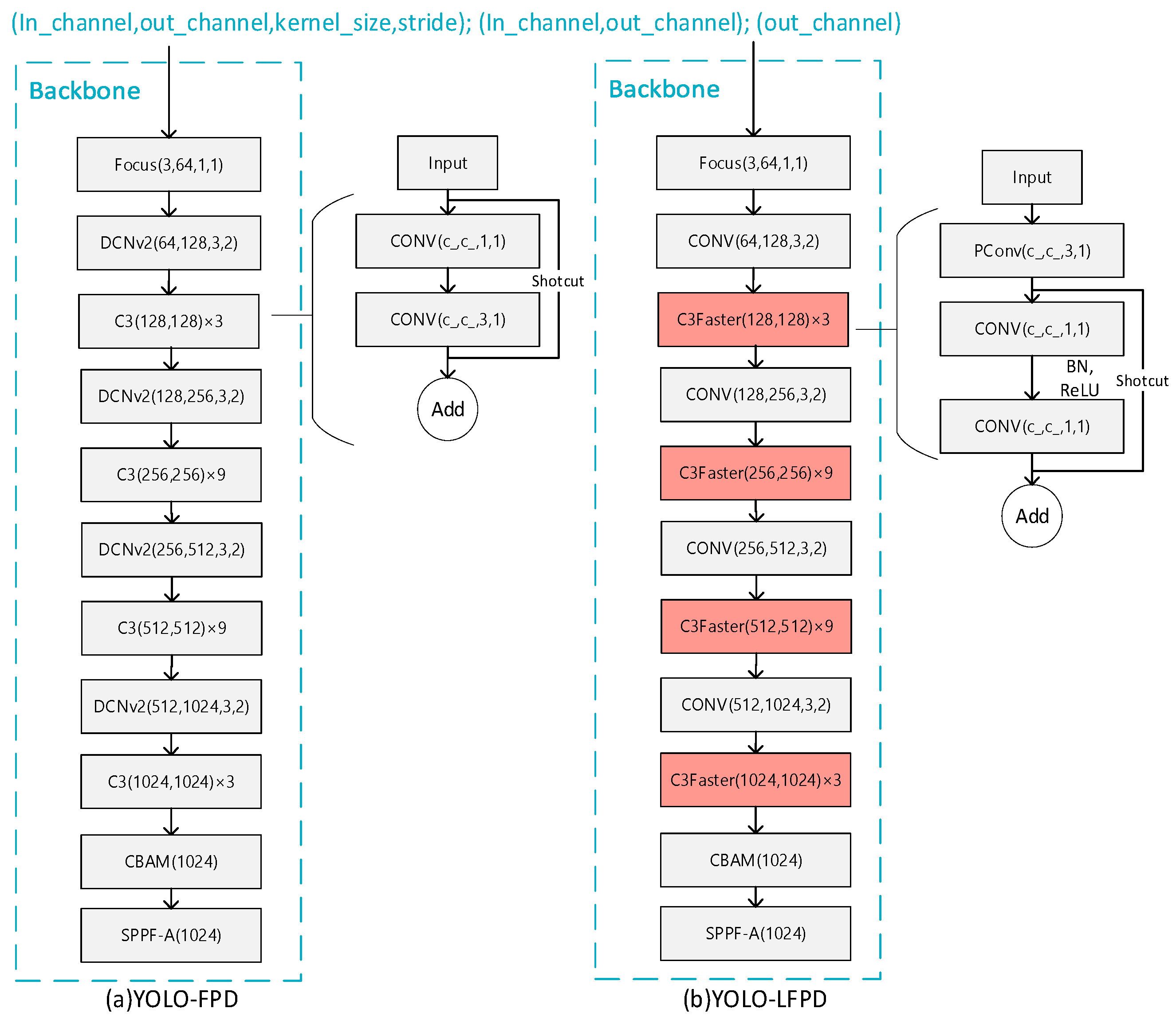
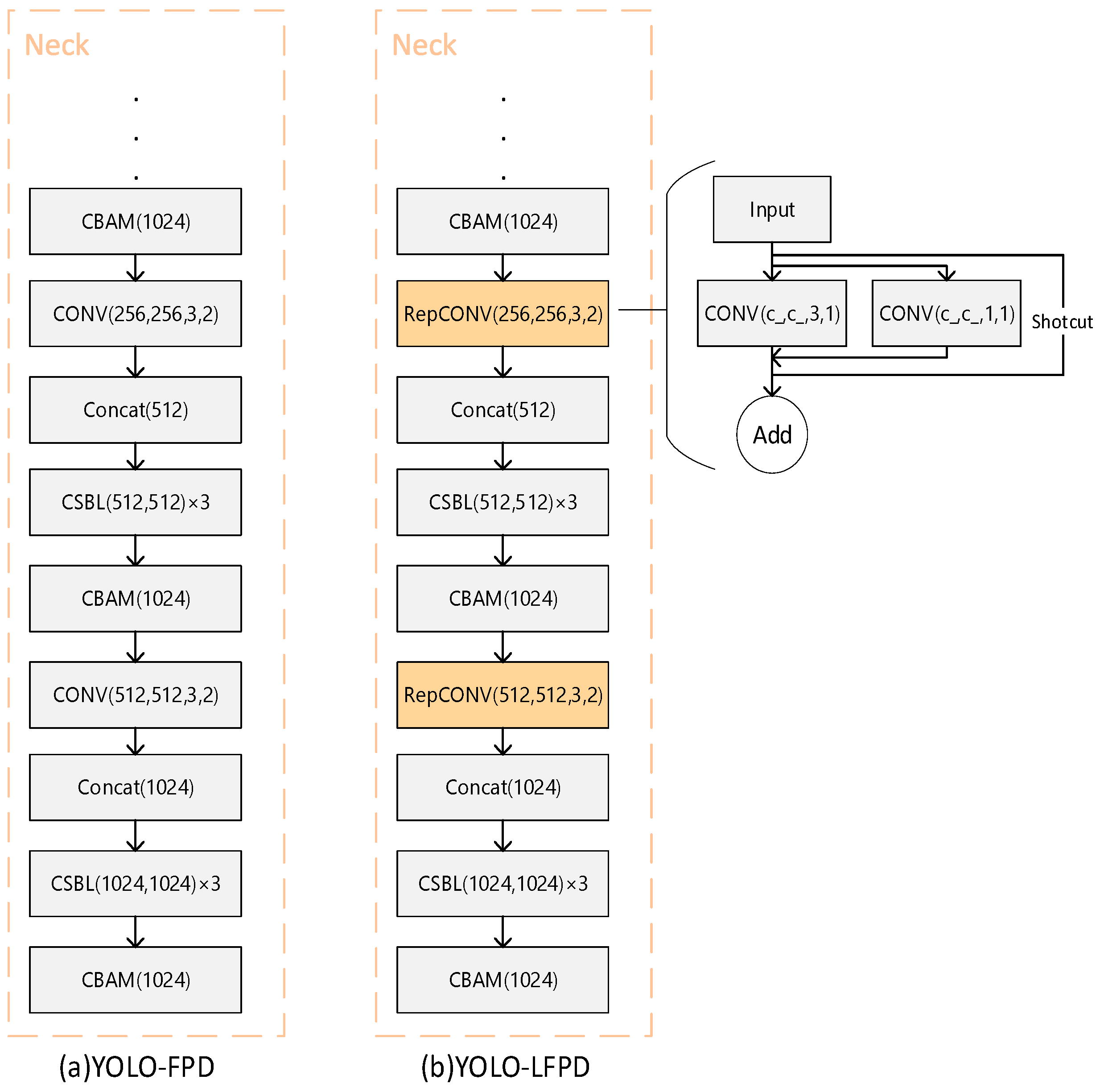
- The RepVGG module simplifies the inference process while allowing the model to acquire more surface defect feature information, with a 0.8% increase in mAP50 accuracy, which reduces the depth of the model while being able to improve the extraction of surface defect image features from the strip. A better fusion effect was obtained by testing the location of the FasterNet module, with a 0.2% increase in mAP50 accuracy. In addition, the FasterNet module allows the model to ignore unimportant feature information, reducing the amount of computation while preventing model overfitting, and reducing the number of parameters and the amount of computation of the model, with the number of parameters being 63.6% of the original, and the GFLOPs being 73.8% of the original.
- Performance tests were conducted on the NEU dataset, GC10-DET dataset, and PKU-Market-PCB dataset. The experimental results demonstrate that the model’s accuracy and number of parameters in this paper are optimal compared to network models from the past two years. Additionally, the model’s ability to perform inference speed is also noteworthy, providing a reference for the application of surface defect detection of strip steel and the deployment of the model in actual production scenarios. The model serves as a reference for applying and deploying it in real production scenarios.
2. Related Work
2.1. Strip Defect Detection Technology
2.2. Pruning
2.3. Hyperparameter Evolution and the OTA Loss Function
2.4. Datasets
3. Modelling Design
3.1. FasterNet Network
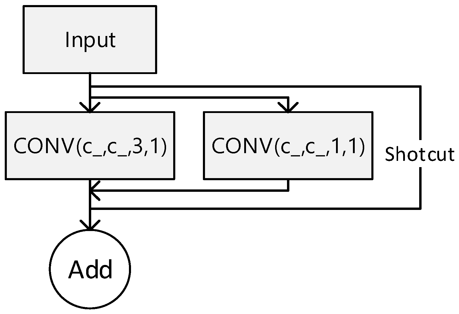
3.2. RepVGG
4. Experiments and Analyses
4.1. Dataset Experiments
4.2. Ablation Experiment
4.3. Experiments on Reasoning Speed
4.4. Fusion Position Experiments
4.5. Parametric Experiments
4.6. Experiment on Pruning
| Algorithm 1 Pruning Judgment Skip Code |
|
|
|
|
4.7. Comparison of Forecast Frames
4.8. Heat Map Comparison
5. Conclusions
- Pruning enables the model to choose the right parameter size for the actual detection, and the mAP50 accuracy still reaches 75.6% when the number of parameters is reduced to half of the original. In addition, the substitution loss function and hyperparameter evolution methods provide a better improvement in accuracy with smaller model parameters, and the mAP50 accuracy is improved by 6.5%.
- The RepVGG module simplifies the inference process while allowing the model to acquire more surface defect feature information, with a 0.8% increase in mAP50 accuracy, which reduces the depth of the model while being able to improve the extraction of surface defect image features from the strip. A better fusion effect was obtained by testing the location of the FasterNet module, with a 0.2% increase in mAP50 accuracy. In addition, the FasterNet module allows the model to ignore unimportant feature information, reducing the amount of computation while preventing model overfitting, and reducing the number of parameters and the amount of computation of the model, with the number of parameters being 63.6% of the original, and the GFLOPs being 73.8% of the original.
- Performance tests were conducted on the NEU dataset, GC10-DET dataset, and PKU-Market-PCB dataset. The experimental results demonstrate that the model’s accuracy and number of parameters in this paper are optimal compared to network models from the past two years. Additionally, the model’s ability to perform inference speed is also noteworthy, providing a reference for the application of surface defect detection of strip steel and the deployment of the model in actual production scenarios. The model serves as a reference for applying and deploying it in real production scenarios.
6. Prospect
- This paper tests the performance of the improved model using the NEU dataset, the GC10-DET dataset, and the PKU-Market-PCB dataset. However, it is important to note that the data images used suffer from an imbalance in the number of labelled types, inaccurate labelling, and omission of labels. Subsequently, it is recommended to utilise GAN and other adversarial networks for image generation to improve and verify the model’s generalisation ability. This will enable the model to detect a wider range of steel surface defects and expand its potential applications.
- This paper focuses solely on detecting surface defects in strip steel and does not extend to other industrial production areas. Future work should explore target detection of surface defects in other workpieces and semantic segmentation of images to enrich research results in the field of steel surface defect detection.
- The lightweight network models proposed in this paper have only been tested on public datasets and have not yet been deployed to mobile or edge devices for real-world performance testing. Future work should focus on testing and validating the models’ performance in real-world scenarios of strip steel surface defect detection after deployment to devices.
Author Contributions
Funding
Institutional Review Board Statement
Data Availability Statement
Acknowledgments
Conflicts of Interest
References
- Platt, J. Sequential Minimal Optimization: A Fast Algorithm for Training Support Vector Machines. 1998. Available online: http://leap.ee.iisc.ac.in/sriram/teaching/MLSP_16/refs/SMO.pdf (accessed on 1 May 2022).
- Rigatti, S.J. Random forest. J. Insur. Med. 2017, 47, 31–39. [Google Scholar] [CrossRef] [PubMed]
- Fukushima, K. Neocognitron: A self-organizing neural network model for a mechanism of pattern recognition unaffected by shift in position. Biol. Cybern. 1980, 36, 193–202. [Google Scholar] [CrossRef]
- He, K.; Gkioxari, G.; Dollár, P.; Girshick, R. Mask r-cnn. In Proceedings of the IEEE International Conference on Computer Vision, Honolulu, HI, USA, 21–26 July 2017; pp. 2961–2969. [Google Scholar]
- Tan, M.; Pang, R.; Le, Q.V. Efficientdet: Scalable and efficient object detection. In Proceedings of the IEEE/CVF Conference on Computer Vision and Pattern Recognition, Seattle, WA, USA, 13–19 June 2020; pp. 10781–10790. [Google Scholar]
- Redmon, J.; Divvala, S.; Girshick, R.; Farhadi, A. You only look once: Unified, real-time object detection. In Proceedings of the IEEE Conference on Computer Vision and Pattern Recognition, Las Vegas, NV, USA, 27–30 June 2016; pp. 779–788. [Google Scholar]
- Ge, Z.; Liu, S.; Wang, F.; Li, Z.; Sun, J. Yolox: Exceeding yolo series in 2021. arXiv 2021, arXiv:2107.08430. [Google Scholar]
- Wang, C.-Y.; Bochkovskiy, A.; Liao, H.-Y.M. YOLOv7: Trainable bag-of-freebies sets new state-of-the-art for real-time object detectors. In Proceedings of the IEEE/CVF Conference on Computer Vision and Pattern Recognition, Vancouver, BC, Canada, 18–22 June 2023; pp. 7464–7475. [Google Scholar]
- Terven, J.; Cordova-Esparza, D. A comprehensive review of YOLO: From YOLOv1 to YOLOv8 and beyond. arXiv 2023, arXiv:2304.00501. [Google Scholar]
- Cañero-Nieto, J.M.; Solano-Martos, J.F.; Martín-Fernández, F. A comparative study of image processing thresholding algorithms on residual oxide scale detection in stainless steel production lines. Procedia Manuf. 2019, 41, 216–223. [Google Scholar] [CrossRef]
- Neogi, N.; Mohanta, D.K.; Dutta, P.K. Defect detection of steel surfaces with global adaptive percentile thresholding of gradient image. J. Inst. Eng. (India) Ser. B 2017, 98, 557–565. [Google Scholar] [CrossRef]
- Li, L.; Hao, P. Steel plate corrugation defect intelligent detection method based on picture cropping and region growing algorithm. In Proceedings of the 2019 14th IEEE Conference on Industrial Electronics and Applications (ICIEA), Xi’an, China, 19–21 June 2019; pp. 587–590. [Google Scholar]
- Chen, Y.; Zhang, J.; Zhang, H. Segmentation algorithm of armor plate surface images based on improved visual attention mechanism. Open Cybern. Syst. J. 2015, 9, 1385–1392. [Google Scholar] [CrossRef]
- Lu, J.; Zhu, M.; Ma, X.; Wu, K. Steel Strip Surface Defect Detection Method Based on Improved YOLOv5s. Biomimetics 2024, 9, 28. [Google Scholar] [CrossRef]
- Liu, R.; Huang, M.; Gao, Z.; Cao, Z.; Cao, P. MSC-DNet: An efficient detector with multi-scale context for defect detection on strip steel surface. Measurement 2023, 209, 112467. [Google Scholar] [CrossRef]
- Zhao, H.; Wan, F.; Lei, G.; Xiong, Y.; Xu, L.; Xu, C.; Zhou, W. LSD-YOLOv5: A Steel Strip Surface Defect Detection Algorithm Based on Lightweight Network and Enhanced Feature Fusion Mode. Sensors 2023, 23, 6558. [Google Scholar] [CrossRef]
- Liang, Y.; Li, J.; Zhu, J.; Du, R.; Wu, X.; Chen, B. A Lightweight Network for Defect Detection in Nickel-Plated Punched Steel Strip Images. IEEE Trans. Instrum. Meas. 2023, 72, 3505515. [Google Scholar] [CrossRef]
- Zhou, X.; Wei, M.; Li, Q.; Fu, Y.; Gan, Y.; Liu, H.; Ruan, J.; Liang, J. Surface Defect Detection of Steel Strip with Double Pyramid Network. Appl. Sci. 2023, 13, 1054. [Google Scholar] [CrossRef]
- Wang, H.; Yang, X.; Zhou, B.; Shi, Z.; Zhan, D.; Huang, R.; Lin, J.; Wu, Z.; Long, D. Strip Surface Defect Detection Algorithm Based on YOLOv5. Materials 2023, 16, 2811. [Google Scholar] [CrossRef] [PubMed]
- Chen, H.; Du, Y.; Fu, Y.; Zhu, J.; Zeng, H. DCAM-Net: A Rapid Detection Network for Strip Steel Surface Defects Based on Deformable Convolution and Attention Mechanism. IEEE Trans. Instrum. Meas. 2023, 72, 5005312. [Google Scholar] [CrossRef]
- Wang, X.; Zhuang, K. An improved YOLOX method for surface defect detection of steel strips. In Proceedings of the 2023 IEEE 3rd International Conference on Power, Electronics and Computer Applications (ICPECA), Shenyang, China, 29–31 January 2023; pp. 152–157. [Google Scholar]
- Xi-Xing, L.; Rui, Y.; Hong-Di, Z. A YOLOv5s-GC-based surface defect detection method of strip steel. Steel Res. Int. 2024, 95, 2300421. [Google Scholar]
- Lee, J.; Park, S.; Mo, S.; Ahn, S.; Shin, J. Layer-adaptive Sparsity for the Magnitude-based Pruning. In Proceedings of the International Conference on Learning Representations, Addis Ababa, Ethiopia, 30 April 2020. [Google Scholar]
- Liu, Z.; Li, J.; Shen, Z.; Huang, G.; Yan, S.; Zhang, C. Learning Efficient Convolutional Networks through Network Slimming. In Proceedings of the 2017 IEEE International Conference on Computer Vision (ICCV), Venice, Italy, 22–29 October 2017; pp. 2755–2763. [Google Scholar]
- Friedman, J.H.; Hastie, T.J.; Tibshirani, R. A note on the group lasso and a sparse group lasso. arXiv 2010, arXiv:1001.0736. [Google Scholar]
- Fang, G.; Ma, X.; Song, M.; Mi, M.B.; Wang, X. DepGraph: Towards Any Structural Pruning. In Proceedings of the 2023 IEEE/CVF Conference on Computer Vision and Pattern Recognition (CVPR), Vancouver, BC, Canada, 18–22 June 2023; pp. 16091–16101. [Google Scholar]
- Wang, H.; Qin, C.; Zhang, Y.; Fu, Y.R. Neural Pruning via Growing Regularization. arXiv 2020, arXiv:2012.09243. [Google Scholar]
- Molchanov, P.; Mallya, A.; Tyree, S.; Frosio, I.; Kautz, J. Importance Estimation for Neural Network Pruning. In Proceedings of the 2019 IEEE/CVF Conference on Computer Vision and Pattern Recognition (CVPR), Long Beach, CA, USA, 15–20 June 2019; pp. 11256–11264. [Google Scholar]
- Filters’Importance, D. Pruning Filters for Efficient ConvNets. 2016. Available online: http://asim.ai/papers/ecnn_poster.pdf (accessed on 1 May 2022).
- Lv, X.; Duan, F.; Jiang, J.-j.; Fu, X.; Gan, L. Deep metallic surface defect detection: The new benchmark and detection network. Sensors 2020, 20, 1562. [Google Scholar] [CrossRef]
- Yu, X.; Lyu, W.; Zhou, D.; Wang, C.; Xu, W. ES-Net: Efficient scale-aware network for tiny defect detection. IEEE Trans. Instrum. Meas. 2022, 71, 3511314. [Google Scholar] [CrossRef]
- Qin, R.; Chen, N.; Huang, Y. EDDNet: An efficient and accurate defect detection network for the industrial edge environment. In Proceedings of the 2022 IEEE 22nd International Conference on Software Quality, Reliability and Security (QRS), Guangzhou, China, 5–9 December 2022; pp. 854–863. [Google Scholar]
- Li, Z.; Wei, X.; Hassaballah, M.; Jiang, X. A One-Stage Deep Learning Model for Industrial Defect Detection. Adv. Theory Simul. 2023, 6, 2200853. [Google Scholar] [CrossRef]
- Shao, R.; Zhou, M.; Li, M.; Han, D.; Li, G. TD-Net: Tiny defect detection network for industrial products. Complex Intell. Syst. 2024, 10, 3943–3954. [Google Scholar] [CrossRef]
- Huang, Z.; Zhang, C.; Ge, L.; Chen, Z.; Lu, K.; Wu, C. Joining Spatial Deformable Convolution and a Dense Feature Pyramid for Surface Defect Detection. IEEE Trans. Instrum. Meas. 2024, 73, 5012614. [Google Scholar] [CrossRef]
- Xie, Y.; Hu, W.; Xie, S.; He, L. Surface defect detection algorithm based on feature-enhanced YOLO. Cogn. Comput. 2023, 15, 565–579. [Google Scholar] [CrossRef]
- Zhang, L.; Chen, J.; Chen, J.; Wen, Z.; Zhou, X. LDD-Net: Lightweight printed circuit board defect detection network fusing multi-scale features. Eng. Appl. Artif. Intell. 2024, 129, 107628. [Google Scholar] [CrossRef]
- Chen, J.; Kao, S.-h.; He, H.; Zhuo, W.; Wen, S.; Lee, C.-H.; Chan, S.-H.G. Run, Don’t Walk: Chasing Higher FLOPS for Faster Neural Networks. In Proceedings of the IEEE/CVF Conference on Computer Vision and Pattern Recognition, Vancouver, BC, Canada, 18–22 June 2023; pp. 12021–12031. [Google Scholar]
- Qian, X.; Wang, X.; Yang, S.; Lei, J. LFF-YOLO: A YOLO Algorithm With Lightweight Feature Fusion Network for Multi-Scale Defect Detection. IEEE Access 2022, 10, 130339–130349. [Google Scholar] [CrossRef]
- Hung, M.-H.; Ku, C.-H.; Chen, K.-Y. Application of Task-Aligned Model Based on Defect Detection. Automation 2023, 4, 327–344. [Google Scholar] [CrossRef]
- Ma, H.; Zhang, Z.; Zhao, J. A Novel ST-YOLO Network for Steel-Surface-Defect Detection. Sensors 2023, 23, 9152. [Google Scholar] [CrossRef]
- Guo, Z.; Wang, C.; Yang, G.; Huang, Z.; Li, G. Msft-yolo: Improved yolov5 based on transformer for detecting defects of steel surface. Sensors 2022, 22, 3467. [Google Scholar] [CrossRef]
- Kou, X.; Liu, S.; Cheng, K.; Qian, Y. Development of a YOLO-V3-based model for detecting defects on steel strip surface. Measurement 2021, 182, 109454. [Google Scholar] [CrossRef]
- Zhao, C.; Shu, X.; Yan, X.; Zuo, X.; Zhu, F. RDD-YOLO: A modified YOLO for detection of steel surface defects. Measurement 2023, 214, 112776. [Google Scholar] [CrossRef]
- Huang, Y.; Tan, W.; Li, L.; Wu, L. WFRE-YOLOv8s: A New Type of Defect Detector for Steel Surfaces. Coatings 2023, 13, 2011. [Google Scholar] [CrossRef]
- Zeng, Q.; Wei, D.; Zhang, X.; Gan, Q.; Wang, Q.; Zou, M. MFAM-Net: A Surface Defect Detection Network for Strip Steel via Multiscale Feature Fusion and Attention Mechanism. In Proceedings of the 2023 International Conference on New Trends in Computational Intelligence (NTCI), Qingdao, China, 3–5 November 2023; pp. 117–121. [Google Scholar]
- Tang, J.; Liu, S.; Zhao, D.; Tang, L.; Zou, W.; Zheng, B. PCB-YOLO: An improved detection algorithm of PCB surface defects based on YOLOv5. Sustainability 2023, 15, 5963. [Google Scholar] [CrossRef]
- Du, B.; Wan, F.; Lei, G.; Xu, L.; Xu, C.; Xiong, Y. YOLO-MBBi: PCB surface defect detection method based on enhanced YOLOv5. Electronics 2023, 12, 2821. [Google Scholar] [CrossRef]
- Mantravadi, A.; Makwana, D.; Mittal, S.; Singhal, R. Dilated Involutional Pyramid Network (DInPNet): A Novel Model for Printed Circuit Board (PCB) Components Classification. In Proceedings of the 2023 24th International Symposium on Quality Electronic Design (ISQED), San Francisco, CA, USA, 5–7 April 2023; pp. 1–7. [Google Scholar]
- Wu, Y.; He, K. Group normalization. In Proceedings of the European Conference on Computer Vision (ECCV), Munich, Germany, 8–14 September 2018; pp. 3–19. [Google Scholar]


| Typology | Training Set | Validation Set | Test Set | Subtotal |
|---|---|---|---|---|
| leakage holes | 76 | 23 | 16 | 115 |
| open circuits | 79 | 24 | 6 | 109 |
| rat bites | 86 | 27 | 9 | 122 |
| short circuits | 87 | 16 | 13 | 116 |
| stray copper | 79 | 26 | 10 | 115 |
| stray | 78 | 22 | 16 | 116 |
| Experimental Environment | Configuration Parameters |
|---|---|
| CPU | Intel(R)i5-12400 |
| GPU | NVIDIA 3060 (12 GB) |
| Deep Learning Frameworks | Pytorch3.8 |
| Programming Language | Python3.7 |
| GPU Acceleration Library | CUDA11.2 CUDNN11.2 |
| Model | mAP@0.5 | AP(%) | Model Parameter | |||||
|---|---|---|---|---|---|---|---|---|
| Cr | In | Ps | Pa | Rs | Sc | |||
| SDD [39] | 67.1 | 38.2 | 72.1 | 72.0 | 87.9 | 65.3 | 66.9 | 93.2 M params, 116.3 GFLOPs |
| Faster R-CNN | 71.3 | 37.6 | 80.2 | 81.5 | 85.3 | 54.0 | 89.2 | - |
| ES-Net [39] | 79.1 | 60.9 | 82.5 | 95.8 | 94.3 | 67.2 | 74.1 | 148.0 M params |
| LDD-Net [37] | 74.4 | − | − | − | − | − | − | 21.5 GFLOPs |
| Efficiendet [39] | 70.1 | 45.9 | 62.0 | 85.5 | 83.5 | 70.7 | 73.1 | 199.4 M params, 12.6 GFLOPs |
| DEA-RetinaNet [39] | 79.1 | 60.1 | 82.5 | 95.8 | 94.3 | 67.2 | 74.1 | 168.8 M params |
| DCC-CenterNet [39] | 79.4 | 45.7 | 90.6 | 82.5 | 85.1 | 76.8 | 95.8 | 131.2 M params |
| YOLOv3 [39] | 69.9 | 28.1 | 74.6 | 78.7 | 91.6 | 54.1 | 92.5 | 236.3 M params, 33.1 GFLOPs |
| TAMD [40] | 77.9 | 56.8 | 82.8 | 82.6 | 92.0 | 60.5 | 92.4 | − |
| TD-Net [34] | 76.8 | − | − | − | − | − | − | − |
| YOLOv5n | 76.0 | 40.1 | 87.3 | 82.7 | 90.4 | 64.0 | 91.4 | 280 layer, 3 M params, 4.3 GFLOPs, 6.7 MB |
| YOLOv5s | 77.3 | 46.1 | 82.2 | 87.8 | 91.1 | 64.9 | 91.8 | 280 layers, 12.3 M params, 16.2 GFLOPs, 25.2 MB |
| YOLOv7-Tiny | 72.4 | 37.0 | 82.8 | 82.3 | 87.8 | 55.5 | 89.0 | 263 layers, 6 M params, 13.2 GFLOPs, 12.3 MB |
| YOLOv7 | 73.4 | 36.8 | 85.6 | 80.7 | 88.1 | 58.7 | 90.4 | 415 layers, 37.2 M params, 104.8 GFLOPs, 74.9 MB |
| DEA-RetinaNet [39] | 79.1 | 60.1 | 82.5 | 95.8 | 94.3 | 67.2 | 74.1 | 168.8 M params |
| DCC-CenterNet [39] | 79.4 | 45.7 | 90.6 | 82.5 | 85.1 | 76.8 | 95.8 | 131.2 M params |
| YOLOv3 [39] | 69.9 | 28.1 | 74.6 | 78.7 | 91.6 | 54.1 | 92.5 | 236.3 M params, 33.1 GFLOPs |
| YOLOX [41] | 77.1 | 46.6 | 83.1 | 83.5 | 88.6 | 64.8 | 95.7 | – 9 M params, 26.8 GFLOPs, 71.8 MB |
| LFF-YOLO [39] | 79.23 | 45.1 | 85.5 | 86.3 | 94.5 | 67.8 | 96.1 | – 6.85 M params, 60.5 GFLOPs, – |
| MSFT-YOLO [42] | 75.2 | 56.9 | 80.8 | 82.1 | 93.5 | 52.7 | 83.5 | – |
| YOLO-V3-based model [43] | 72.2 | – | – | – | – | – | – | – |
| ST-YOLO [41] | 80.3 | 54.6 | 83.0 | 84.7 | 89.2 | 73.2 | 97.0 | 55.8 M params, |
| RDD-YOLO [44] | 81.1 | – | – | – | – | – | – | – |
| YOLOv8s | 74.7 | 43.6 | 82.2 | 78.1 | 94.0 | 66.8 | 83.3 | 225 layers, 11.1 M params, 28.4 GFLOPs, 21.5 MB |
| WFRE-YOLOv8s [45] | 79.4 | 60.0 | 81.4 | 82.5 | 93.8 | 73.8 | 84.8 | 13.8 M params, 32.6 GFLOPs |
| YOLO-FPD | 79.6 | 56.2 | 83.0 | 88.4 | 87.5 | 69.4 | 93.2 | 232 layers, 13.2 M params, 20.2 GFLOPs, 25.4 MB |
| YOLO-LFPD-n | 78.3 | 50.4 | 81.7 | 86.7 | 89.7 | 72.4 | 89.2 | 238 layers, 1.6 M params, 3.8 GFLOPs, 3.3 MB |
| YOLO-LFPD | 81.2 | 63.0 | 82.4 | 89.8 | 86.5 | 71.9 | 93.9 | 238 layers, 6.4 M params, 14.1 GFLOPs, 12.5 MB |
| Model | mAP@0.5 | Model Parameter |
|---|---|---|
| YOLOv5s | 65.5 | 280 layers, 12.3 M params, 16.2 GFLOPs, 25.2 MB |
| LSD-YOLOv5 [16] | 67.9 | 2.7 M params, 9.1 GFLOPs |
| MFAM-Net [46] | 66.7 | − |
| TD-Net [34] | 71.5 | − |
| Improved YOLOX [21] | 70.5 | − |
| WFRE-YOLOv8s [45] | 69.4 | 13.8 M params, 32.6 GFLOPs |
| YOLO-LFPD | 72.8 | 238 layers, 6.4 M params, 14.1 GFLOPs, 12.5 MB |
| Model | mAP@0.5 | Model Parameter |
|---|---|---|
| Tiny RetinaNet [47] | 70.0 | − |
| EfficientDet [47] | 69.0 | − |
| TDD-Net [48] | 95.1 | − |
| YOLOX [47] | 92.3 | 9 M params, 26.8 GFLOPs, 71.8 MB |
| YOLOv5s | 94.7 | 280 layers, 12.3 M params, 16.2 GFLOPs, 25.2 MB |
| YOLOv7 [48] | 95.3 | 415 layers, 37.2 M params, 104.8 GFLOPs, 74.9 MB |
| YOLO-MBBi [48] | 95.3 | − |
| PCB-YOLO [47] | 96.0 | − |
| DInPNet [49] | 95.5 | − |
| TD-Net [34] | 96.2 | − |
| YOLO-LFPD | 98.2 | 238 layers, 6.4 M params, 14.1 GFLOPs, 12.5 MB |
| Model | mAP@0.5 | Params | GFLOPs |
|---|---|---|---|
| YOLO-FPD | 79.6 | 13.2 M | 20.2 |
| YOLO-FPD + FasterNet | 79.8 | 8.4 M | 14.9 |
| YOLO-FPD + RepVGG | 80.4 | 11.2 M | 19.4 |
| YOLO-LFPD | 81.2 | 6.4 M | 14.1 |
| Model | mAP@0.5 | Parameter/M | GFLOPs | Speed of Reasoning/ms |
|---|---|---|---|---|
| YOLOv5n | 76.0 | 3 | 4.3 | 3.8 |
| YOLOv5s | 77.3 | 12.3 | 16.2 | 7.0 |
| YOLOv7-Tiny | 72.4 | 6 | 13.2 | 9.0 |
| YOLOv7 | 73.4 | 37.2 | 104.8 | 9.5 |
| YOLOv8s | 74.7 | 11.1 | 28.4 | 7.5 |
| YOLO-FPD | 79.6 | 13.2 | 20.2 | 7.2 |
| YOLO-LFPD-n | 78.3 | 1.6 (53%) | 3.8 (88%) | 3.2 (84%) |
| YOLO-LFPD | 81.2 | 6.4 (52%) | 14.1 (87%) | 5.4 (77%) |
| Fusion Position | mAP@0.5 | FPS |
|---|---|---|
| Backbone Network | 79.8 | 139 |
| Neck Network | 79.5 | 137 |
| Detection Heads | 79.3 | 136 |
| Model | mAP@0.5 | mAP@0.95 |
|---|---|---|
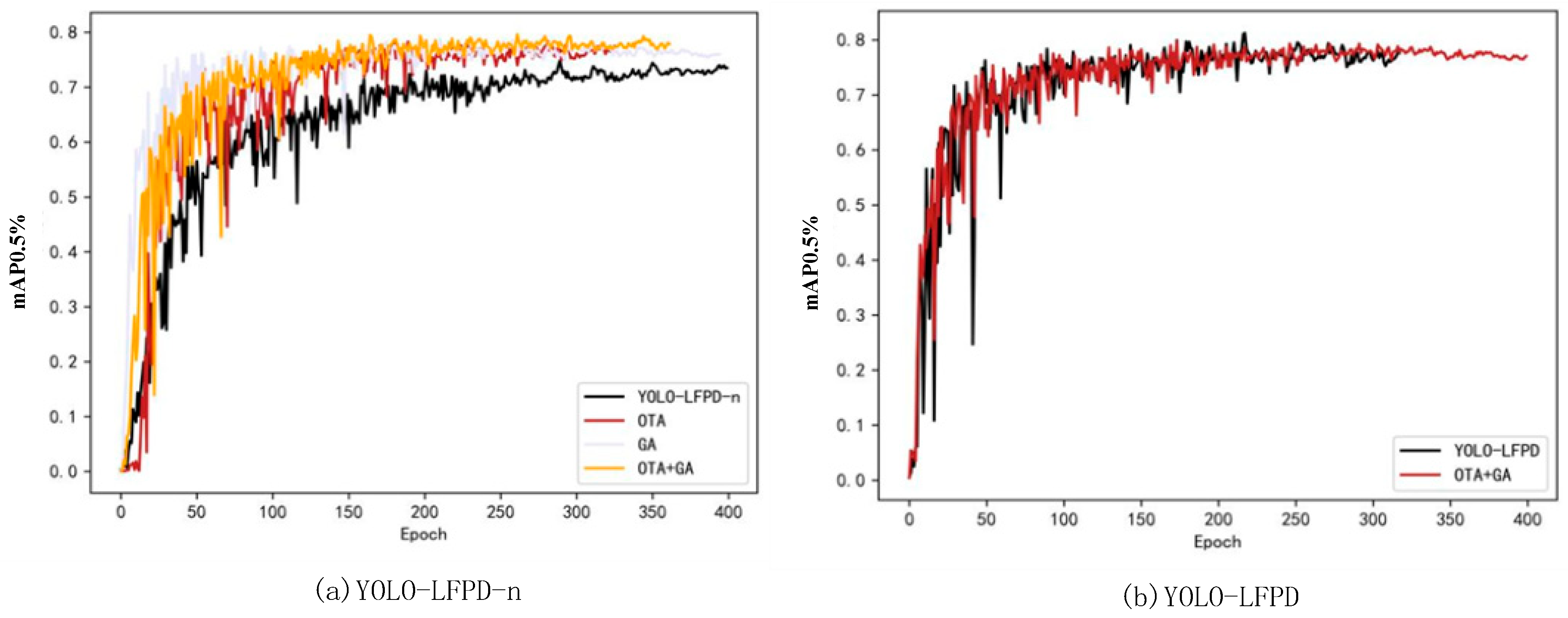
| YOLO-LFPD-n | 74.0 | 40.9 |
| OTA + YOLO-LFPD-n | 77.6 | 42.5 |
| GA + YOLO-LFPD-n | 77.4 | 43.0 |
| OTA + GA + YOLO-LFPD-n | 78.3 | 43.2 |
| OTA + GA + YOLO-LFPD | 80.5 | 44.4 |
| YOLO-LFPD | 81.2 | 44.3 |
| Pruning Method | GFLOPs | Model Size/MB | Parameter/M | mAP@0.5 |
|---|---|---|---|---|
| YOLO-LFPD | 3.5 | 12.5 | 6.4 | 81.2 |
| L1-1.5× | 2.6 | 8.5 | 4.3 | 77.3 |
| L1-2.0× | 1.72 | 6.4 | 3.17 | 75.6 |
| SLIM-1.5× | 2.6 | 8.5 | 12.3 | 68.4 |
| SLIM-2.0× | 1.71 | 6.4 | 3.16 | 64.5 |
| SLIM-4.0× | 0.88 | 3.3 | 1.66 | 61.4 |
| LAMP-1.5× | 2.6 | 8.5 | 4.31 | 71.8 |
| LAMP-2.0× | 1.72 | 6.4 | 3.17 | 72.9 |
| LAMP-4.0× | 0.88 | 3.3 | 1.66 | 70.4 |
| Group_slim-1.5× | 2.6 | 8.5 | 4.3 | 74.0 |
| Group_slim-2.0× | 1.72 | 6.4 | 3.16 | 70.6 |
| Group_taylor-1.5× | 2.6 | 8.5 | 4.3 | 73.1 |
| Group_taylor-2.0× | 1.72 | 6.4 | 3.16 | 71.4 |
| Growing_reg1.2× | 2.91 | 10.7 | 5.37 | 74.1 |
| Growing_reg1.5× | 2.6 | 8.5 | 4.3 | 74.7 |
| Group_norm1.2× | 2.9 | 10.4 | 5.37 | 75.8 |
| Group_norm1.4× | 2.5 | 8.9 | 4.56 | 77.1 |
| Group_norm1.5× | 2.6 | 8.5 | 4.31 | 77.4 |
| Group_norm-2.0× | 1.72 | 6.4 | 3.16 | 75.3 |
Disclaimer/Publisher’s Note: The statements, opinions and data contained in all publications are solely those of the individual author(s) and contributor(s) and not of MDPI and/or the editor(s). MDPI and/or the editor(s) disclaim responsibility for any injury to people or property resulting from any ideas, methods, instructions or products referred to in the content. |
© 2024 by the authors. Licensee MDPI, Basel, Switzerland. This article is an open access article distributed under the terms and conditions of the Creative Commons Attribution (CC BY) license (https://creativecommons.org/licenses/by/4.0/).
Share and Cite
Lu, J.; Zhu, M.; Qin, K.; Ma, X. YOLO-LFPD: A Lightweight Method for Strip Surface Defect Detection. Biomimetics 2024, 9, 607. https://doi.org/10.3390/biomimetics9100607
Lu J, Zhu M, Qin K, Ma X. YOLO-LFPD: A Lightweight Method for Strip Surface Defect Detection. Biomimetics. 2024; 9(10):607. https://doi.org/10.3390/biomimetics9100607
Chicago/Turabian StyleLu, Jianbo, Mingrui Zhu, Kaixian Qin, and Xiaoya Ma. 2024. "YOLO-LFPD: A Lightweight Method for Strip Surface Defect Detection" Biomimetics 9, no. 10: 607. https://doi.org/10.3390/biomimetics9100607
APA StyleLu, J., Zhu, M., Qin, K., & Ma, X. (2024). YOLO-LFPD: A Lightweight Method for Strip Surface Defect Detection. Biomimetics, 9(10), 607. https://doi.org/10.3390/biomimetics9100607