
Path Planning of Unmanned Aerial Vehicles Based on an Improved Bio-Inspired Tuna Swarm Optimization Algorithm

Abstract
1. Introduction
- (1)
- A mathematical model was established by reviewing existing drone path optimization strategies.
- (2)
- A new unmanned aerial vehicle path optimization strategy was created using an improved tuna optimization algorithm, and it was improved through sine and Levy’s flight.
- (3)
- The simulation results were used to confirm the efficiency and effectiveness of the proposed technology.
- (4)
- The performance indicators of the proposed algorithm were compared with seven other algorithms.
2. Relate Works
3. Mathematical Model for Path Planning of UAVs
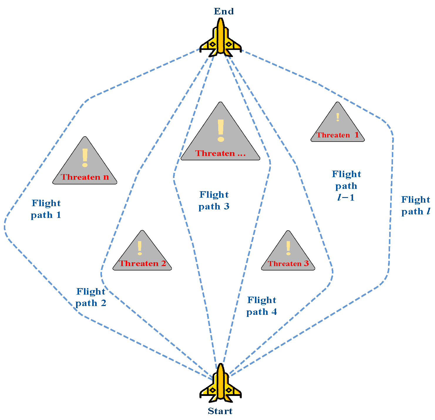
3.1. The Problem with Trajectory Planning
3.2. Path Encoding
3.3. Constraint Condition
3.4. Optimization Objectives
3.4.1. Fuel Consumption
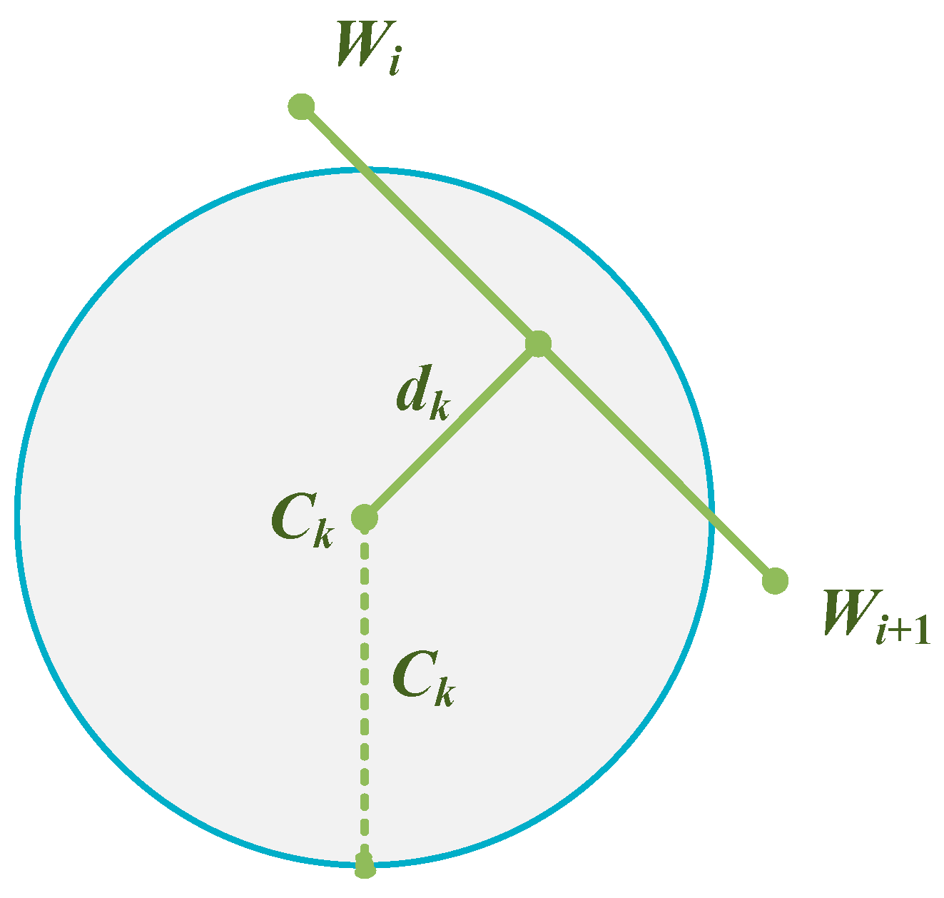
3.4.2. Threats
3.5. Path Planning Model for UAVs
4. Tuna Swarm Optimization Algorithm (TSO)
Standard Tuna Swarm Optimization Algorithm (TSO)
- (1)
- Population Initialization
- (2)
- Tuna school spiral feeding
- (3)
- Tuna parabolic foraging
5. Improved TSO Algorithm Based on the Sine Strategy and Levy Flight (SLTSO)
5.1. Elite Opposition-Based Learning Mechanism
5.2. Introducing the Levy Flight Strategy and the Greedy Strategy to Update Positions
5.3. Introducing the Golden Sine Strategy to Update Individual Positions
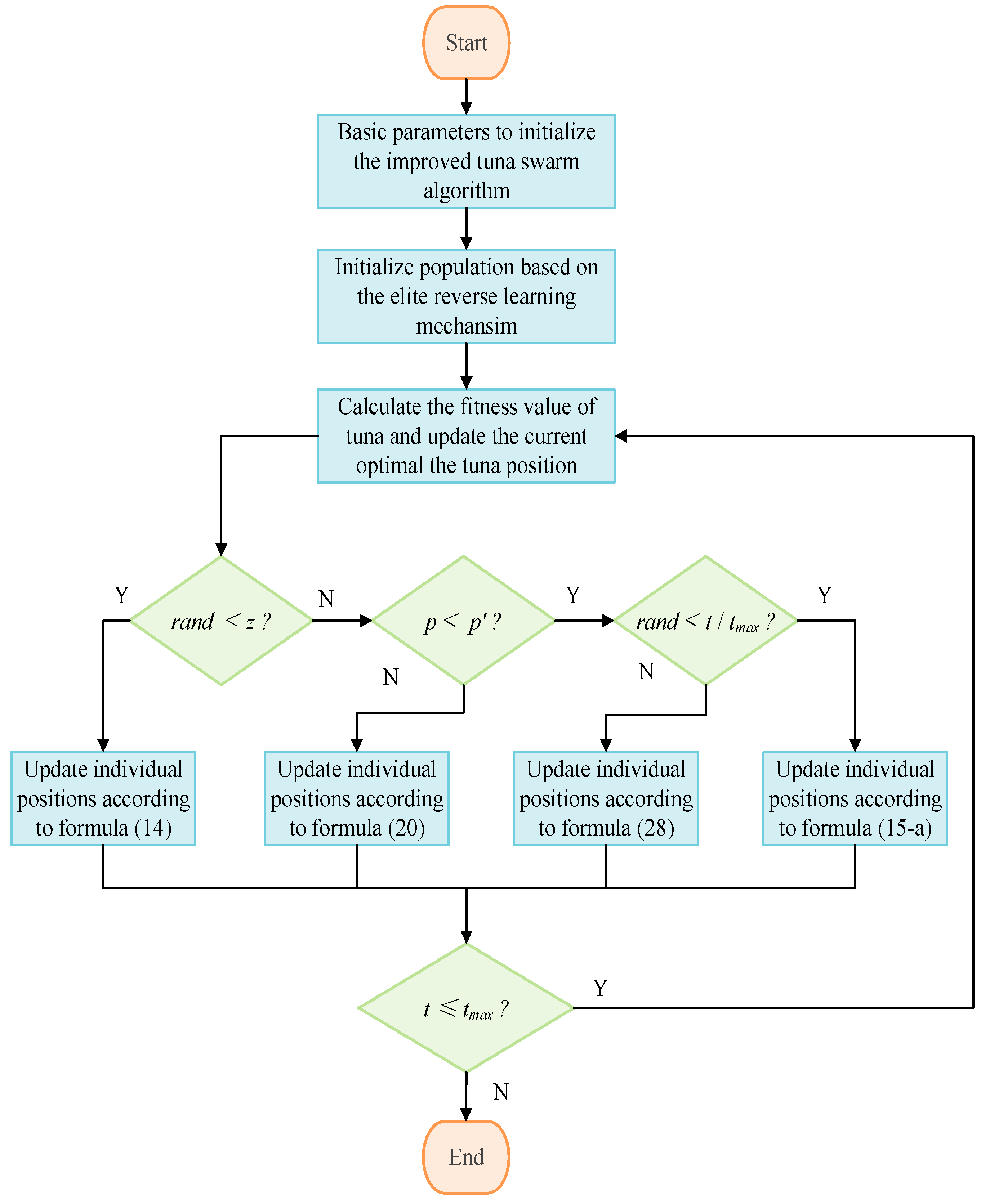
5.4. The Workflow for the Proposed SLTSO Algorithm
5.5. Time Complexity Analysis of the SLTSO Algorithm
6. Simulation Experiments and Result Analysis
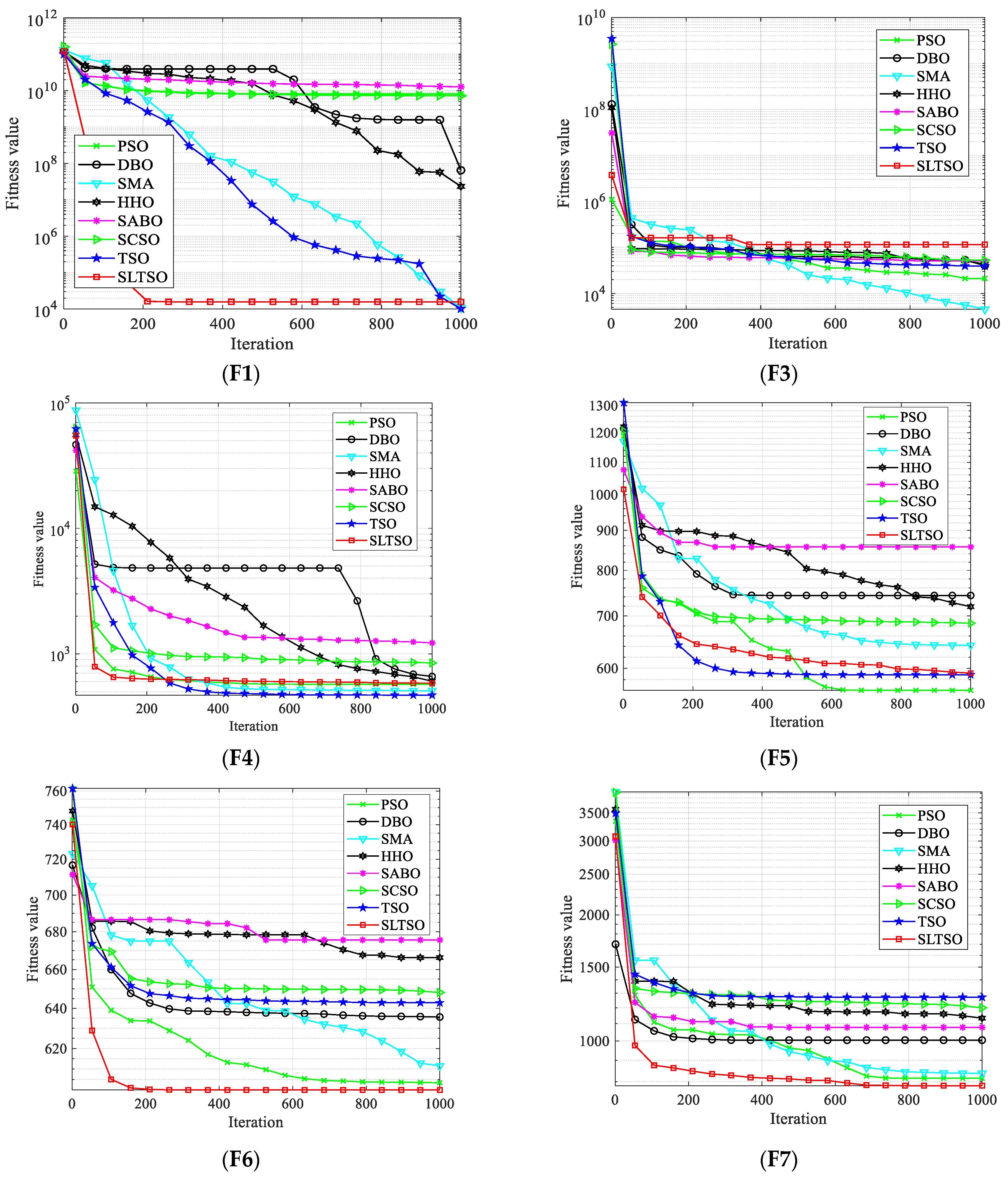
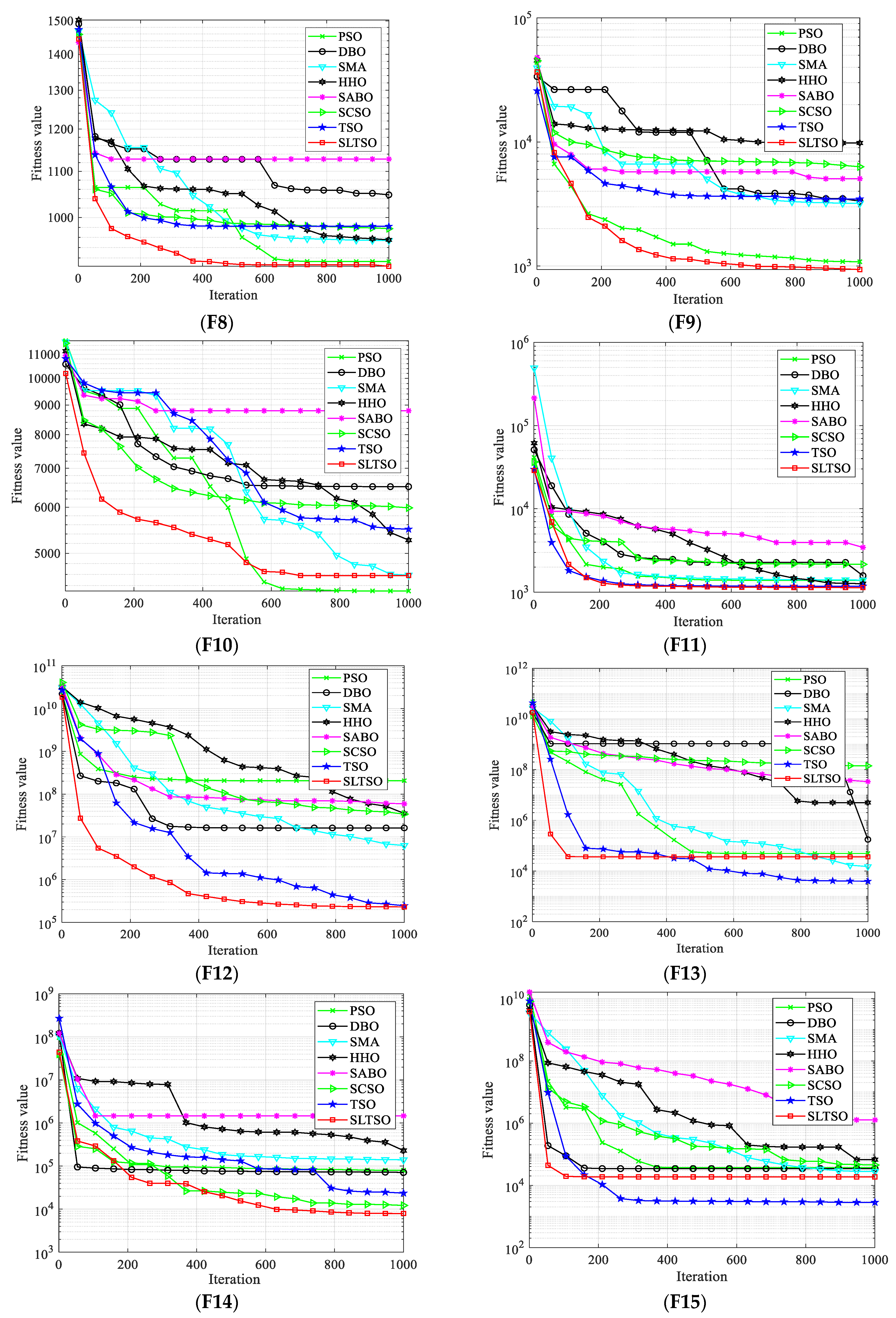
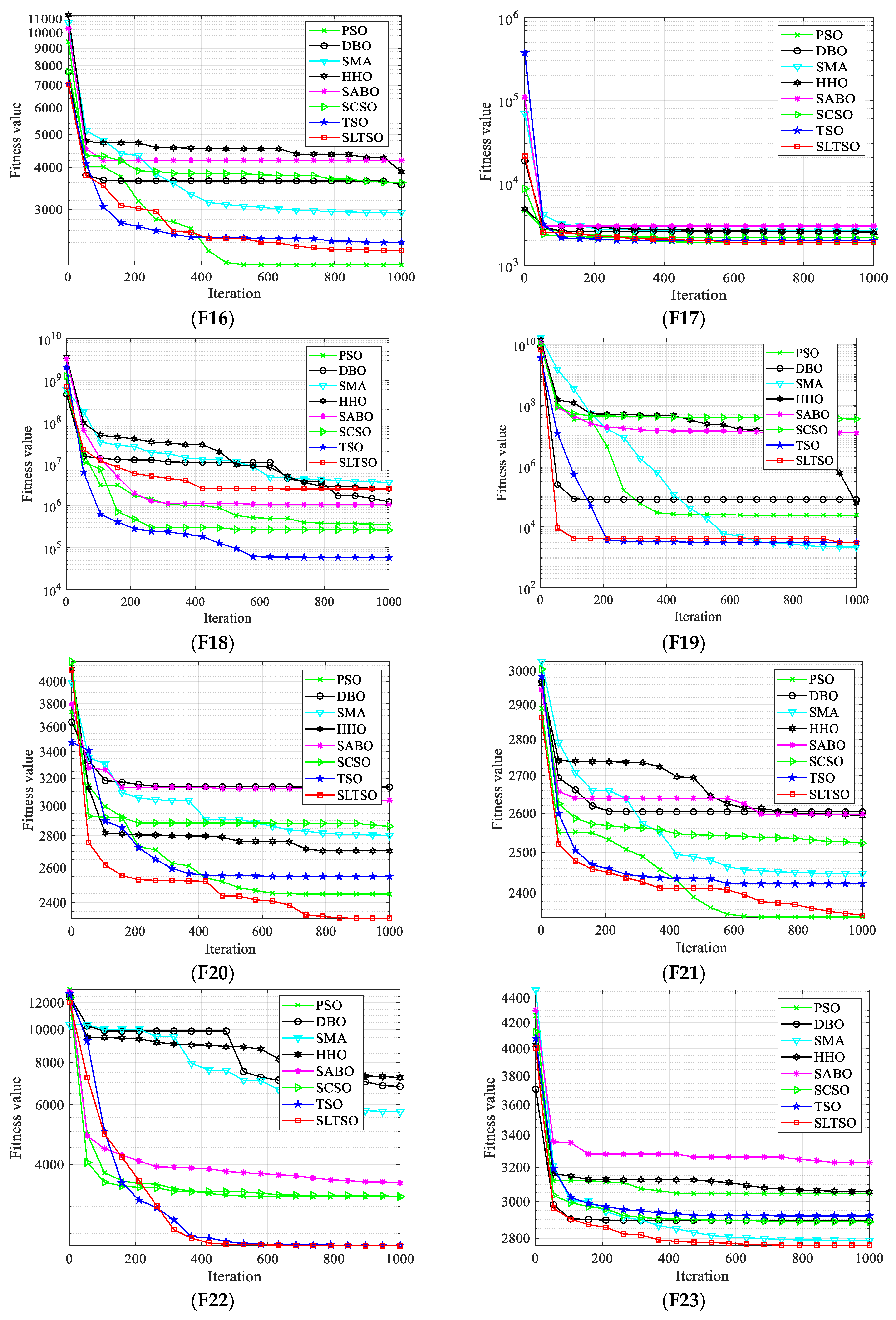
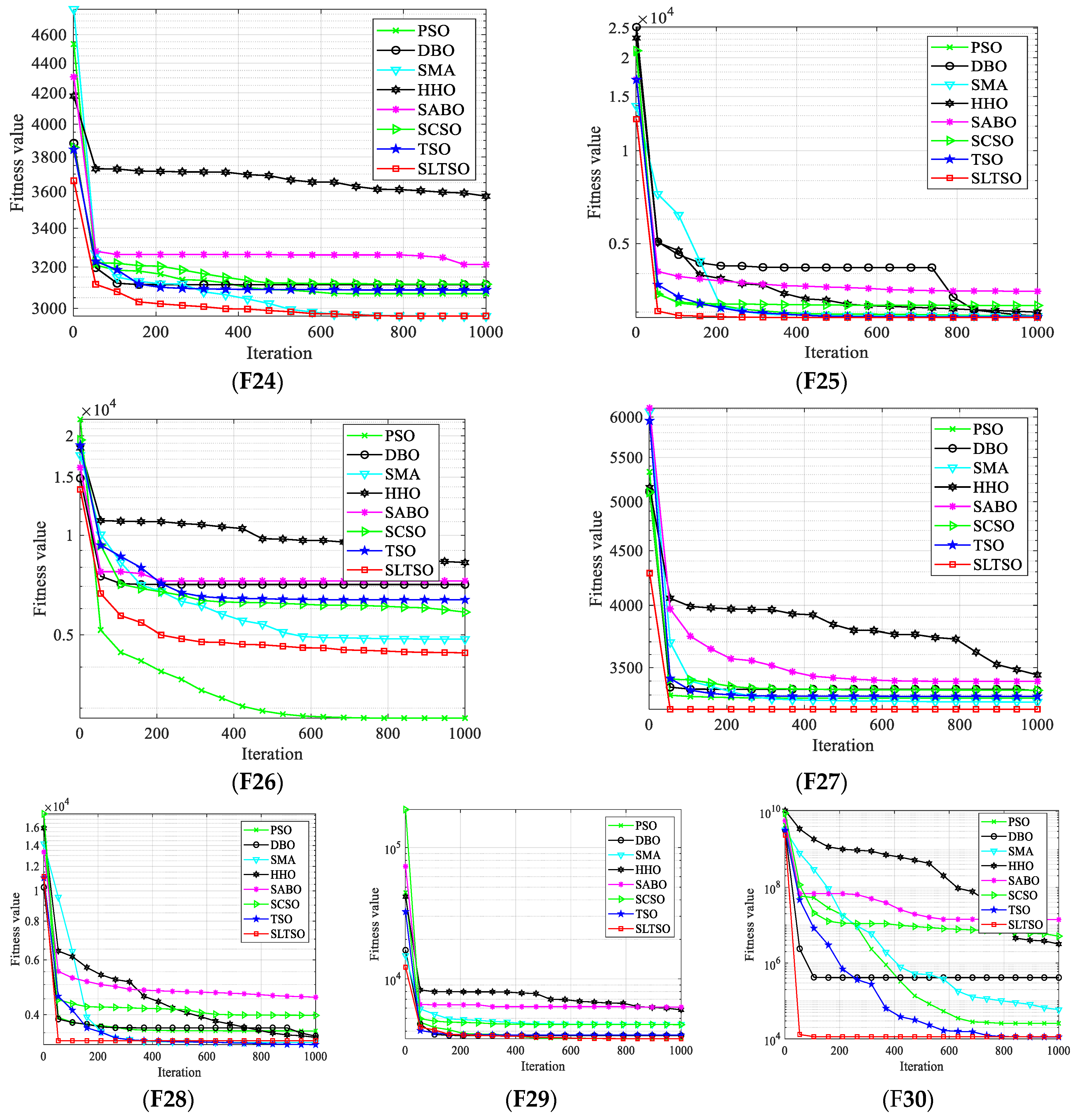
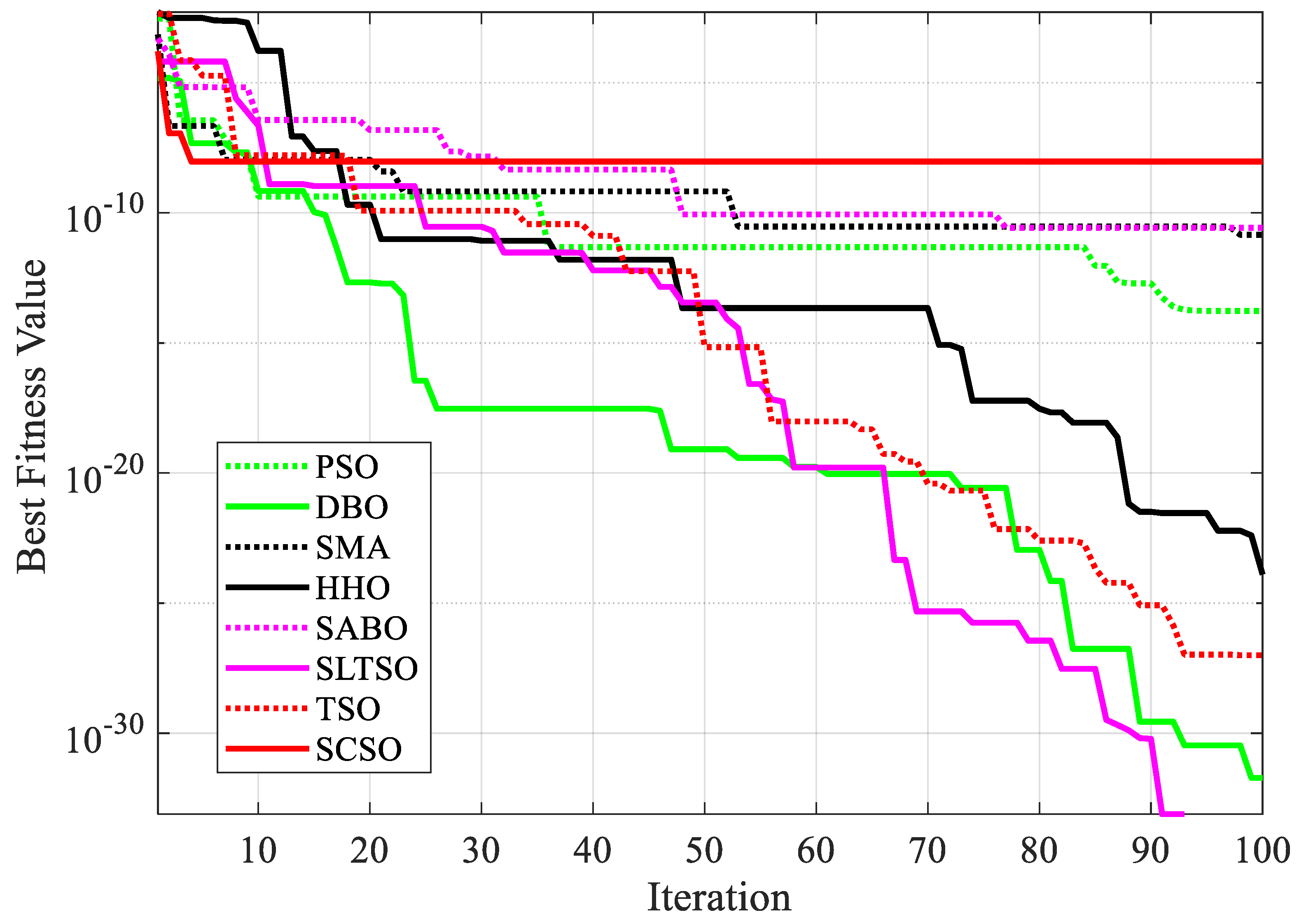
6.1. Comparison of Test Function Results
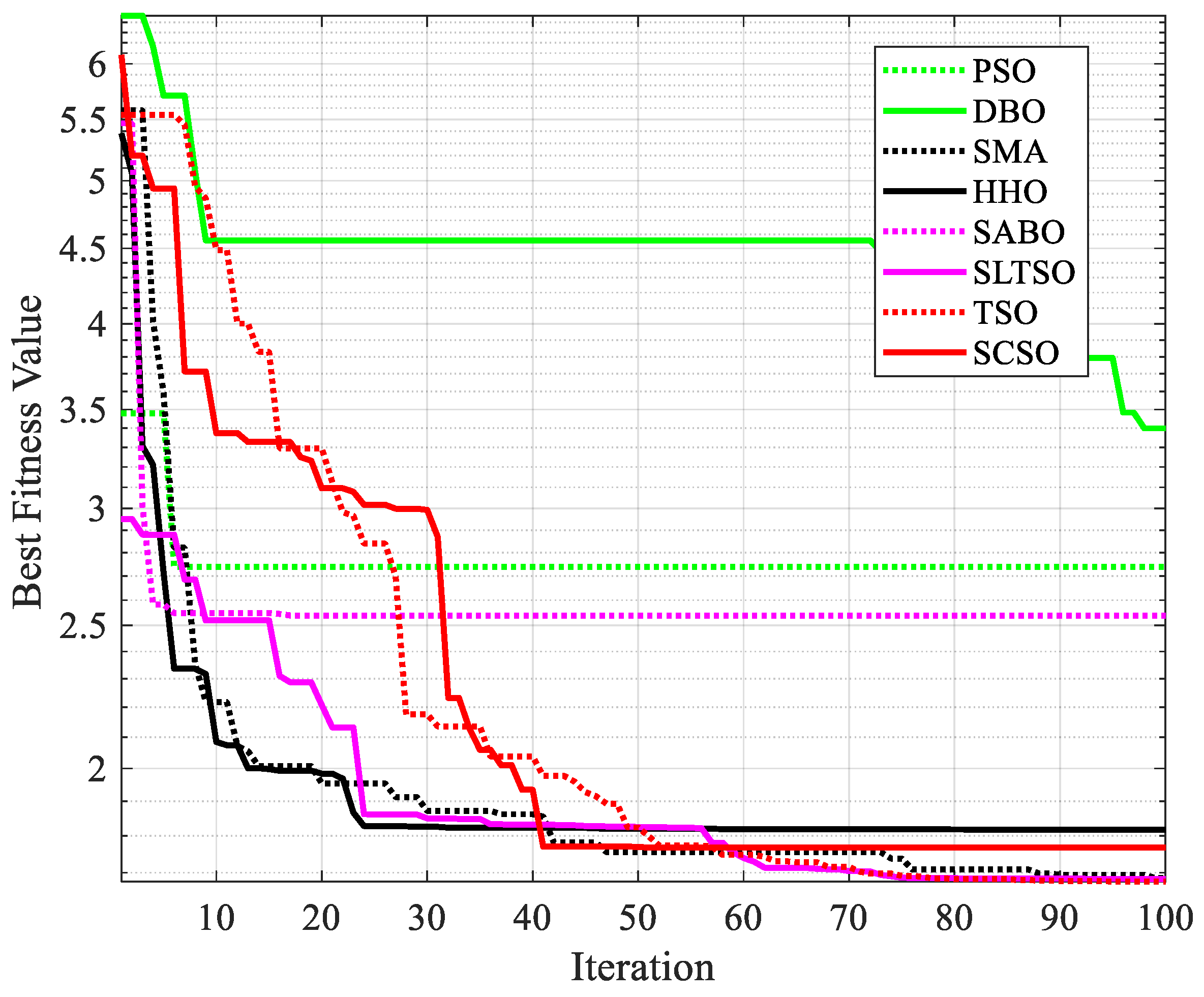
6.2. Comparison of Engineering Application
- (1)
- Welding beam design problem
- (2)
- Gear train design problem
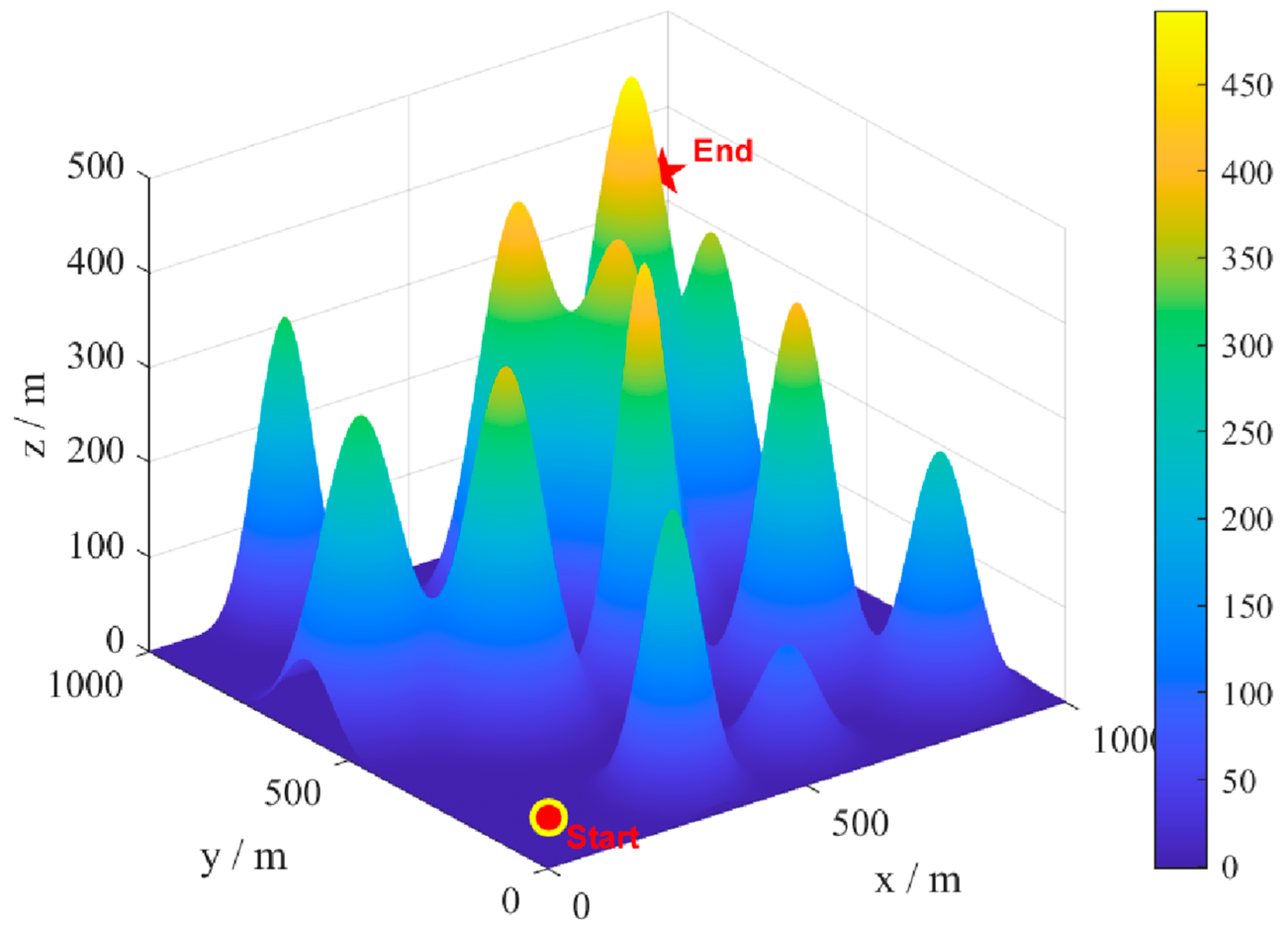
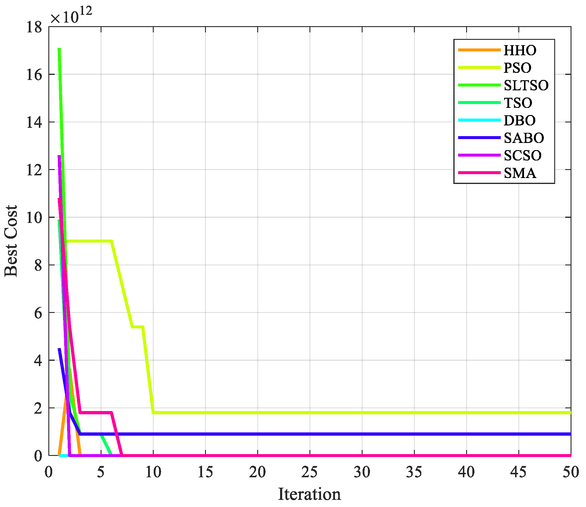
6.3. Comparison of UAV Path Planning
7. Conclusions
Author Contributions
Funding
Institutional Review Board Statement
Data Availability Statement
Conflicts of Interest
References
- Jones, M.; Djahel, S.; Welsh, K. Path-planning for unmanned aerial vehicles with environment complexity considerations: A survey. ACM Comput. Surv. 2023, 55, 1–39. [Google Scholar] [CrossRef]
- Jayaweera, H.M.P.C.; Hanoun, S. Path planning of unmanned aerial vehicles (UAVs) in windy environments. Drones 2022, 6, 101. [Google Scholar] [CrossRef]
- Shahid, N.; Abrar, M.; Ajmal, U.; Masroor, R.; Amjad, S.; Jeelani, M. Path planning in unmanned aerial vehicles: An optimistic overview. Int. J. Commun. Syst. 2022, 35, e5090. [Google Scholar] [CrossRef]
- Maheswaran, S.; Murugesan, G.; Duraisamy, P.; Vivek, B.; Selvapriya, S.; Vinith, S.; Vasantharajan, V. Unmanned ground vehicle for surveillance. In Proceedings of the 2020 11th International Conference on Computing, Communication and Networking Technologies (ICCCNT), Kharagpur, India, 1–3 July 2020; IEEE: Piscataway, NJ, USA, 2020; pp. 1–5. [Google Scholar]
- Wang, J.; Zhao, Z.; Qu, J.; Chen, X. APPA-3D: An autonomous 3D path planning algorithm for UAVs in unknown complex environments. Sci. Rep. 2024, 14, 1231. [Google Scholar] [CrossRef]
- Guo, Y.; Liu, X.; Zhang, W.; Yang, Y. 3D path planning method for UAV based on improved artificial potential field. Xibei Gongye Daxue Xuebao J. Northwestern Polytech. Univ. 2020, 38, 977–986. [Google Scholar] [CrossRef]
- Lee, S.; Yu, H.; Lee, H. Multiagent Q-learning-based multi-UAV wireless networks for maximizing energy efficiency: Deployment and power control strategy design. IEEE Internet Things J. 2021, 9, 6434–6442. [Google Scholar] [CrossRef]
- Zhao, Y.; Zheng, Z.; Liu, Y. Survey on computational-intelligence-based UAV path planning. Knowl.-Based Syst. 2018, 158, 54–64. [Google Scholar] [CrossRef]
- Tang, W.; Cao, L.; Chen, Y.; Yue, Y. Solving Engineering Optimization Problems Based on Multi-Strategy Particle Swarm Optimization Hybrid Dandelion Optimization Algorithm. Biomimetics 2024, 9, 298. [Google Scholar] [CrossRef]
- Yue, Y.; Cao, L.; Lu, D.; Hu, Z.; Xu, M.; Wang, S.; Li, B.; Ding, H. Review and empirical analysis of sparrow search algorithm. Artif. Intell. Rev. 2023, 56, 10867–10919. [Google Scholar] [CrossRef]
- Cao, L.; Chen, H.; Chen, Y.; Yue, Y.; Zhang, X. Bio-Inspired Swarm Intelligence Optimization Algorithm-Aided Hybrid TDOA/AOA-Based Localization. Biomimetics 2023, 8, 186. [Google Scholar] [CrossRef] [PubMed]
- Wang, S.; Cao, L.; Chen, Y.; Chen, C.; Yue, Y.; Zhu, W. Gorilla optimization algorithm combining sine cosine and cauchy variations and its engineering applications. Sci. Rep. 2024, 14, 7578. [Google Scholar] [CrossRef] [PubMed]
- Yue, Y.; Cao, L.; Chen, H.; Chen, Y.; Su, Z. Towards an Optimal KELM Using the PSO-BOA Optimization Strategy with Applications in Data Classification. Biomimetics 2023, 8, 306. [Google Scholar] [CrossRef] [PubMed]
- Cao, L.; Wang, Z.; Wang, Z.; Wang, X.; Yue, Y. An Energy-Saving and Efficient Deployment Strategy for Heterogeneous Wireless Sensor Networks Based on Improved Seagull Optimization Algorithm. Biomimetics 2023, 8, 231. [Google Scholar] [CrossRef] [PubMed]
- Chen, B.; Cao, L.; Chen, C.; Chen, Y.; Yue, Y. A comprehensive survey on the chicken swarm optimization algorithm and its applications: State-of-the-art and research challenges. Artif. Intell. Rev. 2024, 57, 170. [Google Scholar] [CrossRef]
- Zhu, H.; Wang, Y.; Li, X. UCAV path planning for avoiding obstacles using cooperative co-evolution spider monkey optimization. Knowl.-Based Syst. 2022, 246, 108713. [Google Scholar] [CrossRef]
- Shi, J.; Li, T.; Zhang, H.; Lian, X.; Xu, T. Adaptive multi-UAV path planning method based on improved gray wolf algorithm. Comput. Electr. Eng. 2022, 104, 108377. [Google Scholar]
- Awad, A.; Kamel, S.; Hassan, M.H.; Mohamed, F. An enhanced tuna swarm algorithm for optimizing FACTS and wind turbine allocation in power systems. Electr. Power Compon. Syst. 2024, 52, 863–878. [Google Scholar] [CrossRef]
- Yan, Z.; Yan, J.; Wu, Y.; Cai, S.; Wang, H. A novel reinforcement learning based tuna swarm optimization algorithm for autonomous underwater vehicle path planning. Math. Comput. Simul. 2023, 209, 55–86. [Google Scholar] [CrossRef]
- Lv, J.X.; Yan, L.J.; Chu, S.C.; Cai, Z.M.; Pan, J.S.; He, X.K.; Xue, J.K. A new hybrid algorithm based on golden eagle optimizer and grey wolf optimizer for 3D path planning of multiple UAVs in power inspection. Neural Comput. Appl. 2022, 34, 11911–11936. [Google Scholar] [CrossRef]
- Kiani, F.; Seyyedabbasi, A.; Nematzadeh, S.; Candan, F.; Çevik, T.; Anka, F.A.; Randazzo, G.; Lanza, S.; Muzirafuti, A. Adaptive metaheuristic-based methods for autonomous robot path planning: Sustainable agricultural applications. Appl. Sci. 2022, 12, 943. [Google Scholar] [CrossRef]
- Liu, X.; Li, G.; Yang, H.; Zhang, N.; Wang, L.; Shao, P. Agricultural UAV trajectory planning by incorporating multi-mechanism improved grey wolf optimization algorithm. Expert Syst. Appl. 2023, 233, 120946. [Google Scholar] [CrossRef]
- Jarray, R.; Al-Dhaifallah, M.; Rezk, H.; Bouallègue, S. Parallel cooperative coevolutionary grey wolf optimizer for path planning problem of unmanned aerial vehicles. Sensors 2022, 22, 1826. [Google Scholar] [CrossRef] [PubMed]
- Feng, J.; Sun, C.; Zhang, J.; Du, Y.; Liu, Z.; Ding, Y. A UAV Path Planning Method in Three-Dimensional Space Based on a Hybrid Gray Wolf Optimization Algorithm. Electronics 2023, 13, 68. [Google Scholar] [CrossRef]
- Kumar, R.; Singh, L.; Tiwari, R. Novel Reinforcement Learning Guided Enhanced Variable Weight Grey Wolf Optimization (RLV-GWO) Algorithm for Multi-UAV Path Planning. Wirel. Pers. Commun. 2023, 131, 2093–2123. [Google Scholar] [CrossRef]
- Kelner, J.M.; Burzynski, W.; Stecz, W. Modeling UAV swarm flight trajectories using Rapidly-exploring Random Tree algorithm. J. King Saud Univ. Comput. Inf. Sci. 2024, 36, 101909. [Google Scholar] [CrossRef]
- Cao, L.; Wang, L.; Liu, Y.; Yan, S. 3D trajectory planning based on the Rapidly-exploring Random Tree–Connect and artificial potential fields method for unmanned aerial vehicles. Int. J. Adv. Robot. Syst. 2022, 19, 17298806221118867. [Google Scholar] [CrossRef]
- Blasi, L.; D’Amato, E.; Mattei, M.; Notaro, I. Uav path planning in 3d constrained environments based on layered essential visibility graphs. IEEE Trans. Aerosp. Electron. Syst. 2022, 59, 2359–2375. [Google Scholar] [CrossRef]
- Chowdhury, A.; De, D. RGSO-UAV: Reverse Glowworm Swarm Optimization inspired UAV path-planning in a 3D dynamic environment. Ad Hoc Netw. 2023, 140, 103068. [Google Scholar] [CrossRef]
- Phung, M.D.; Ha, Q.P. Safety-enhanced UAV path planning with spherical vector-based particle swarm optimization. Appl. Soft Comput. 2021, 107, 107376. [Google Scholar] [CrossRef]
- Wang, B.H.; Wang, D.B.; Ali, Z.A. A Cauchy mutant pigeon-inspired optimization–based multi-unmanned aerial vehicle path planning method. Meas. Control 2020, 53, 83–92. [Google Scholar] [CrossRef]
- Saeed, R.A.; Omri, M.; Abdel-Khalek, S.; Ali, E.S.; Alotaibi, M.F. Optimal path planning for drones based on swarm intelligence algorithm. Neural Comput. Appl. 2022, 34, 10133–10155. [Google Scholar] [CrossRef]
- Gugan, G.; Haque, A. Path planning for autonomous drones: Challenges and future directions. Drones 2023, 7, 169. [Google Scholar] [CrossRef]
- Vazquez-Carmona, E.V.; Vasquez-Gomez, J.I.; Herrera-Lozada, J.C.; Antonio-Cruz, M. Coverage path planning for spraying drones. Comput. Ind. Eng. 2022, 168, 108125. [Google Scholar] [CrossRef]
- Li, L.L.; Ji, B.X.; Lim, M.K.; Tseng, M.L. Active distribution network operational optimization problem: A multi-objective tuna swarm optimization model. Appl. Soft Comput. 2024, 150, 111087. [Google Scholar] [CrossRef]
- Xie, L.; Han, T.; Zhou, H.; Zhang, Z.-R.; Han, B.; Tang, A. Tuna swarm optimization: A novel swarm-based metaheuristic algorithm for global optimization. Comput. Intell. Neurosci. 2021, 2021, 9210050. [Google Scholar] [CrossRef]
- Fan, C.; Wang, W.; Tian, J. Flexible job shop scheduling with stochastic machine breakdowns by an improved tuna swarm optimization algorithm. J. Manuf. Syst. 2024, 74, 180–197. [Google Scholar] [CrossRef]
- Fu, C.; Zhang, L. A novel method based on tuna swarm algorithm under complex partial shading conditions in PV system. Sol. Energy 2022, 248, 28–40. [Google Scholar] [CrossRef]
- Gou, Y.; Guo, C.; He, M.; Jiang, Y. A Method for Predicting Typical Characteristics of Voltage Sags Based on TSO-XGBoost Algorithm. In Proceedings of the 2023 2nd Asian Conference on Frontiers of Power and Energy (ACFPE), Chengdu, China, 20–22 October 2023; IEEE: Piscataway, NJ, USA, 2023; pp. 99–103. [Google Scholar]
- Nanda, B.; Muni, B.P.; Jena, R.K. Enhancing Power Quality in Microgrids with Hybrid Tuna-Glowworm Swarm Optimization Strategy for Renewable Energy Sources. Energy Technol. 2023, 12, 2300067. [Google Scholar] [CrossRef]
- Sheeja, R.; Iqbal, M.M.; Sivasankar, C. Multi-objective-derived energy efficient routing in wireless sensor network using adaptive black hole-tuna swarm optimization strategy. Ad Hoc Netw. 2023, 144, 103140. [Google Scholar] [CrossRef]
- Sun, C.; Shao, Q.; Zhou, Z.; Zhang, J. An Enhanced FCM Clustering Method Based on Multi-Strategy Tuna Swarm Optimization. Mathematics 2024, 12, 453. [Google Scholar] [CrossRef]
- Guo, S.M.; Guo, J.K.; Gao, Y.G.; Guo, P.Y.; Wang, S.C.; Lou, Z.C.; Zhang, X. Research on engine speed control based on tuna swarm optimization. J. Eng. Res. Rep. 2022, 23, 272–280. [Google Scholar] [CrossRef]
- Xiao, R.; Liu, G.; Yi, D.; Liu, B.; Zhuang, Q. Study on prediction model of liquid holdup based on back propagation neural network optimized by tuna swarm algorithm. Energy Sources Part A Recovery Util. Environ. Eff. 2023, 45, 8623–8641. [Google Scholar] [CrossRef]
- Yao, Y.; Li, H.; Zeng, Z.; Wang, C.; Zhang, Y. Clustering Routing Protocol Based on Tuna Swarm Optimization and Fuzzy Control Theory in Wireless Sensor Networks. IEEE Sens. J. 2024, 24, 17102–17115. [Google Scholar] [CrossRef]
- Sihwail, R.; Omar, K.; Ariffin, K.A.Z.; Tubishat, M. Improved harris hawks optimization using elite opposition-based learning and novel search mechanism for feature selection. IEEE Access 2020, 8, 121127–121145. [Google Scholar] [CrossRef]
- Choi, T.J.; Lee, J.H.; Youn, H.Y.; Ahn, C.W. Adaptive differential evolution with elite opposition-based learning and its application to training artificial neural networks. Fundam. Informaticae 2019, 164, 227–242. [Google Scholar] [CrossRef]
- Kaidi, W.; Khishe, M.; Mohammadi, M. Dynamic levy flight chimp optimization. Knowl.-Based Syst. 2022, 235, 107625. [Google Scholar] [CrossRef]
- Jain, A.; Rao, A.C.S.; Jain, P.K.; Hu, Y.C. Optimized levy flight model for heart disease prediction using CNN framework in big data application. Expert Syst. Appl. 2023, 223, 119859. [Google Scholar] [CrossRef]
- Li, M.; Liu, Z.; Song, H. An improved algorithm optimization algorithm based on RungeKutta and golden sine strategy. Expert Syst. Appl. 2024, 247, 123262. [Google Scholar] [CrossRef]
- Tanyildizi, E.; Demir, G. Golden Sine Algorithm: A Novel Math-Inspired Algorithm. Adv. Electr. Comput. Eng. 2017, 17, 71–78. [Google Scholar] [CrossRef]
- Li, Z. A local opposition-learning golden-sine grey wolf optimization algorithm for feature selection in data classification. Appl. Soft Comput. 2023, 142, 110319. [Google Scholar] [CrossRef]
- Chen, C.; Cao, L.; Chen, Y.; Chen, B.; Yue, Y. A comprehensive survey of convergence analysis of beetle antennae search algorithm and its applications. Artif. Intell. Rev. 2024, 57, 141. [Google Scholar] [CrossRef]
- Shen, Q.; Zhang, D.; Xie, M.; He, Q. Multi-Strategy Enhanced Dung Beetle Optimizer and Its Application in Three-Dimensional UAV Path Planning. Symmetry 2023, 15, 1432. [Google Scholar] [CrossRef]
- Kopar, M.; Yıldız, A.R.; Yıldız, B.S. Optimum design of a composite drone component using slime mold algorithm. Mater. Test. 2023, 65, 1857–1864. [Google Scholar] [CrossRef]
- Shi, H.; Lu, F.; Wu, L.; Yang, G. Optimal trajectories of multi-UAVs with approaching formation for target tracking using improved Harris Hawks optimizer. Appl. Intell. 2022, 52, 14313–14335. [Google Scholar] [CrossRef]
- Mukhtar, R.; Chang, C.Y.; Raja, M.A.Z.; Chaudhary, N.I. Design of intelligent neuro-supervised networks for brain electrical activity rhythms of Parkinson’s disease model. Biomimetics 2023, 8, 322. [Google Scholar] [CrossRef]
- Niu, Y.; Yan, X.; Wang, Y.; Niu, Y. An improved sand cat swarm optimization for moving target search by UAV. Expert Syst. Appl. 2024, 238, 122189. [Google Scholar] [CrossRef]
- Kaveh, A.; Almasi, P.; Khodagholi, A. Optimum design of castellated beams using four recently developed meta-heuristic algorithms. Iran. J. Sci. Technol. Trans. Civ. Eng. 2023, 47, 713–725. [Google Scholar] [CrossRef]
- Marciniec, A.; Sobolak, M.; Połowniak, P. Graphical method for the analysis of planetary gear trains. Alex. Eng. J. 2022, 61, 4067–4079. [Google Scholar] [CrossRef]


| Function | PSO | DBO | SMA | HHO | SABO | SCSO | TSO | SLTSO | |
|---|---|---|---|---|---|---|---|---|---|
| F1 | Min | 1.16 × 10² | 1.02 × 10² | 9.92 × 10² | 3.00 × 10⁵ | 8.98 × 10⁶ | 2.59 × 10⁴ | 1.01 × 10² | 1.05 × 10² |
| Std | 1.28 × 10⁷ | 1.75 × 10⁷ | 3.92 × 10³ | 5.84 × 10⁵ | 6.34 × 10⁸ | 5.55 × 10⁸ | 2.57 × 10³ | 2.03 × 10³ | |
| Mean | 2.34 × 10⁶ | 5.55 × 10⁶ | 7.43 × 10³ | 1.11 × 10⁶ | 4.84 × 10⁸ | 2.79 × 10⁸ | 1.59 × 10³ | 2.05 × 10³ | |
| F3 | Min | 3.00 × 10² | 3.00 × 10² | 3.00 × 10² | 3.06 × 10² | 7.68 × 10² | 3.17 × 10² | 3.00 × 10² | 3.00 × 10² |
| Std | 7.73 × 10⁻¹ | 1.55 × 10³ | 6.75 × 10⁻¹ | 3.12 × 10² | 1.61 × 10³ | 2.49 × 10³ | 1.06 × 100 | 7.02 × 100 | |
| Mean | 3.00 × 10² | 1.37 × 10³ | 3.00 × 10² | 6.16 × 10² | 3.09 × 10³ | 2.87 × 10³ | 3.00 × 10² | 3.02 × 10² | |
| F4 | Min | 4.01 × 10² | 4.01 × 10² | 4.00 × 10² | 4.00 × 10² | 4.07 × 10² | 4.03 × 10² | 4.00 × 10² | 4.00 × 10² |
| Std | 4.21 × 101 | 3.28 × 101 | 3.21 × 101 | 3.54 × 101 | 2.22 × 101 | 3.89 × 101 | 1.30 × 101 | 2.01 × 101 | |
| Mean | 4.23 × 10² | 4.23 × 10² | 4.22 × 10² | 4.27 × 10² | 4.43 × 10² | 4.41 × 10² | 4.06 × 10² | 4.11 × 10² | |
| F5 | Min | 5.05 × 10² | 5.17 × 10² | 5.09 × 10² | 5.24 × 10² | 5.34 × 10² | 5.12 × 10² | 5.12 × 10² | 5.02 × 10² |
| Std | 8.53 × 100 | 1.37 × 101 | 6.52 × 100 | 1.72 × 101 | 1.03 × 101 | 1.55 × 101 | 1.24 × 101 | 2.37 × 100 | |
| Mean | 5.14 × 10² | 5.40 × 10² | 5.20 × 10² | 5.59 × 10² | 5.54 × 10² | 5.41 × 10² | 5.27 × 10² | 5.07 × 10² | |
| F6 | Min | 6.00 × 10² | 6.01 × 10² | 6.00 × 10² | 6.14 × 10² | 6.09 × 10² | 6.03 × 10² | 6.02 × 10² | 6.00 × 10² |
| Std | 2.89 × 10⁻¹ | 8.23 × 100 | 6.09 × 10⁻¹ | 1.25 × 101 | 1.03 × 101 | 1.07 × 101 | 6.83 × 100 | 9.05 × 10⁻⁹ | |
| Mean | 6.00 × 10² | 6.13 × 10² | 6.00 × 10² | 6.42 × 10² | 6.20 × 10² | 6.18 × 10² | 6.11 × 10² | 6.00 × 10² | |
| F7 | Min | 7.13 × 10² | 7.30 × 10² | 7.19 × 10² | 7.62 × 10² | 7.39 × 10² | 7.39 × 10² | 7.22 × 10² | 7.06 × 10² |
| Std | 6.44 × 100 | 1.45 × 101 | 5.96 × 100 | 1.83 × 101 | 1.39 × 101 | 1.68 × 101 | 1.57 × 101 | 3.46 × 100 | |
| Mean | 7.23 × 10² | 7.49 × 10² | 7.29 × 10² | 7.91 × 10² | 7.67 × 10² | 7.68 × 10² | 7.48 × 10² | 7.16 × 10² | |
| F8 | Min | 8.05 × 10² | 8.07 × 10² | 8.05 × 10² | 8.15 × 10² | 8.32 × 10² | 8.18 × 10² | 8.06 × 10² | 8.02 × 10² |
| Std | 4.71 × 100 | 1.58 × 101 | 8.80 × 100 | 8.53 × 100 | 9.17 × 100 | 7.51 × 100 | 7.37 × 100 | 2.10 × 100 | |
| Mean | 8.13 × 10² | 8.37 × 10² | 8.20 × 10² | 8.30 × 10² | 8.49 × 10² | 8.31 × 10² | 8.22 × 10² | 8.07 × 10² | |
| F9 | Min | 9.00 × 10² | 9.02 × 10² | 9.00 × 10² | 9.82 × 10² | 9.18 × 10² | 9.15 × 10² | 9.11 × 10² | 9.00 × 10² |
| Std | 1.16 × 10⁻¹ | 1.14 × 10² | 2.94 × 100 | 2.14 × 10² | 9.53 × 101 | 2.33 × 10² | 7.82 × 101 | 8.29 × 10⁻² | |
| Mean | 9.00 × 10² | 9.98 × 10² | 9.01 × 10² | 1.58 × 10³ | 1.04 × 10³ | 1.12 × 10³ | 9.96 × 10² | 9.00 × 10² | |
| F10 | Min | 1.02 × 10³ | 1.28 × 10³ | 1.14 × 10³ | 1.27 × 10³ | 2.34 × 10³ | 1.37 × 10³ | 1.37 × 10³ | 1.05 × 10³ |
| Std | 2.55 × 10² | 3.10 × 10² | 2.52 × 10² | 3.65 × 10² | 1.98 × 10² | 3.20 × 10² | 3.00 × 10² | 1.71 × 10² | |
| Mean | 1.58 × 10³ | 1.98 × 10³ | 1.59 × 10³ | 2.03 × 10³ | 2.81 × 10³ | 2.08 × 10³ | 1.96 × 10³ | 1.49 × 10³ | |
| F11 | Min | 1.10 × 10³ | 1.11 × 10³ | 1.11 × 10³ | 1.11 × 10³ | 1.14 × 10³ | 1.11 × 10³ | 1.11 × 10³ | 1.10 × 10³ |
| Std | 2.97 × 101 | 1.22 × 10² | 1.04 × 10² | 5.38 × 101 | 1.37 × 10³ | 4.90 × 101 | 2.38 × 101 | 3.01 × 100 | |
| Mean | 1.12 × 10³ | 1.23 × 10³ | 1.21 × 10³ | 1.18 × 10³ | 1.86 × 10³ | 1.16 × 10³ | 1.14 × 10³ | 1.10 × 10³ | |
| F12 | Min | 3.65 × 10³ | 1.93 × 10³ | 6.40 × 10³ | 5.05 × 10⁴ | 1.41 × 10⁵ | 1.79 × 10⁴ | 2.27 × 10³ | 1.98 × 10³ |
| Std | 1.49 × 10⁶ | 5.67 × 10⁶ | 6.24 × 10⁵ | 2.98 × 10⁶ | 1.72 × 10⁶ | 1.95 × 10⁶ | 9.44 × 10³ | 1.20 × 10⁴ | |
| Mean | 2.96 × 10⁵ | 3.41 × 10⁶ | 4.68 × 10⁵ | 2.46 × 10⁶ | 2.01 × 10⁶ | 1.78 × 10⁶ | 9.76 × 10³ | 1.35 × 10⁴ | |
| F13 | Min | 1.38 × 10³ | 1.51 × 10³ | 1.55 × 10³ | 2.45 × 10³ | 3.56 × 10³ | 2.47 × 10³ | 1.58 × 10³ | 1.36 × 10³ |
| Std | 9.29 × 10³ | 1.19 × 10⁴ | 1.24 × 10⁴ | 8.47 × 10³ | 6.16 × 10³ | 1.05 × 10⁴ | 6.04 × 10³ | 1.32 × 10⁴ | |
| Mean | 9.63 × 10³ | 1.45 × 10⁴ | 1.12 × 10⁴ | 1.42 × 10⁴ | 1.30 × 10⁴ | 1.43 × 10⁴ | 1.00 × 10⁴ | 1.24 × 10⁴ | |
| F14 | Min | 1.43 × 10³ | 1.45 × 10³ | 1.43 × 10³ | 1.50 × 10³ | 1.51 × 10³ | 1.46 × 10³ | 1.43 × 10³ | 1.41 × 10³ |
| Std | 8.39 × 10² | 5.29 × 10² | 2.57 × 10³ | 9.72 × 10² | 1.05 × 10³ | 2.03 × 10³ | 3.96 × 101 | 2.49 × 10² | |
| Mean | 1.76 × 10³ | 1.97 × 10³ | 2.16 × 10³ | 2.09 × 10³ | 2.21 × 10³ | 3.48 × 10³ | 1.50 × 10³ | 1.56 × 10³ | |
| F15 | Min | 1.51 × 10³ | 1.63 × 10³ | 1.53 × 10³ | 1.78 × 10³ | 2.75 × 10³ | 1.58 × 10³ | 1.52 × 10³ | 1.51 × 10³ |
| Std | 2.35 × 10³ | 2.45 × 10³ | 3.62 × 10³ | 3.00 × 10³ | 5.27 × 10³ | 1.80 × 10³ | 3.86 × 10² | 7.64 × 10² | |
| Mean | 3.10 × 10³ | 4.34 × 10³ | 5.19 × 10³ | 7.92 × 10³ | 9.55 × 10³ | 4.92 × 10³ | 1.81 × 10³ | 1.86 × 10³ | |
| F16 | Min | 1.60 × 10³ | 1.61 × 10³ | 1.60 × 10³ | 1.63 × 10³ | 1.79 × 10³ | 1.62 × 10³ | 1.60 × 10³ | 1.60 × 10³ |
| Std | 1.37 × 10² | 1.45 × 10² | 9.73 × 101 | 1.49 × 10² | 1.23 × 10² | 1.34 × 10² | 1.19 × 10² | 4.60 × 101 | |
| Mean | 1.76 × 10³ | 1.82 × 10³ | 1.70 × 10³ | 1.93 × 10³ | 2.06 × 10³ | 1.82 × 10³ | 1.79 × 10³ | 1.63 × 10³ | |
| F17 | Min | 1.71 × 10³ | 1.73 × 10³ | 1.72 × 10³ | 1.75 × 10³ | 1.76 × 10³ | 1.73 × 10³ | 1.72 × 10³ | 1.70 × 10³ |
| Std | 3.24 × 101 | 4.04 × 101 | 3.63 × 101 | 5.87 × 101 | 7.79 × 101 | 2.98 × 101 | 2.32 × 101 | 2.49 × 101 | |
| Mean | 1.75 × 10³ | 1.78 × 10³ | 1.76 × 10³ | 1.80 × 10³ | 1.87 × 10³ | 1.77 × 10³ | 1.75 × 10³ | 1.72 × 10³ | |
| F18 | Min | 2.23 × 10³ | 2.18 × 10³ | 4.46 × 10³ | 2.89 × 10³ | 2.55 × 10³ | 4.08 × 10³ | 2.01 × 10³ | 1.97 × 10³ |
| Std | 1.52 × 10⁴ | 1.62 × 10⁴ | 1.40 × 10⁴ | 1.33 × 10⁴ | 1.21 × 10⁴ | 1.77 × 10⁴ | 7.14 × 10³ | 7.76 × 10³ | |
| Mean | 2.27 × 10⁴ | 1.91 × 10⁴ | 2.57 × 10⁴ | 1.89 × 10⁴ | 1.88 × 10⁴ | 2.41 × 10⁴ | 9.01 × 10³ | 8.51 × 10³ | |
| F19 | Min | 1.96 × 10³ | 1.97 × 10³ | 1.93 × 10³ | 1.94 × 10³ | 3.05 × 10³ | 1.95 × 10³ | 1.94 × 10³ | 1.91 × 10³ |
| Std | 6.92 × 10³ | 2.06 × 10⁴ | 1.05 × 10⁴ | 1.87 × 10⁴ | 5.33 × 10³ | 6.89 × 10³ | 7.06 × 10² | 9.75 × 10² | |
| Mean | 6.29 × 10³ | 1.14 × 10⁴ | 1.49 × 10⁴ | 2.08 × 10⁴ | 8.90 × 10³ | 8.01 × 10³ | 2.56 × 10³ | 2.57 × 10³ | |
| F20 | Min | 2.00 × 10³ | 2.03 × 10³ | 2.00 × 10³ | 2.04 × 10³ | 2.12 × 10³ | 2.04 × 10³ | 2.01 × 10³ | 2.00 × 10³ |
| Std | 5.44 × 101 | 7.86 × 101 | 5.01 × 101 | 6.89 × 101 | 6.66 × 101 | 6.78 × 101 | 6.41 × 101 | 2.23 × 101 | |
| Mean | 2.05 × 10³ | 2.12 × 10³ | 2.05 × 10³ | 2.18 × 10³ | 2.23 × 10³ | 2.14 × 10³ | 2.10 × 10³ | 2.01 × 10³ | |
| F21 | Min | 2.20 × 10³ | 2.20 × 10³ | 2.10 × 10³ | 2.20 × 10³ | 2.33 × 10³ | 2.20 × 10³ | 2.20 × 10³ | 2.20 × 10³ |
| Std | 4.09 × 101 | 5.52 × 101 | 5.58 × 101 | 7.04 × 101 | 1.52 × 101 | 5.48 × 101 | 4.02 × 101 | 5.17 × 101 | |
| Mean | 2.30 × 10³ | 2.23 × 10³ | 2.31 × 10³ | 2.32 × 10³ | 2.35 × 10³ | 2.31 × 10³ | 2.22 × 10³ | 2.27 × 10³ | |
| F22 | Min | 2.23 × 10³ | 2.24 × 10³ | 2.22 × 10³ | 2.26 × 10³ | 2.31 × 10³ | 2.30 × 10³ | 2.24 × 10³ | 2.20 × 10³ |
| Std | 2.93 × 101 | 2.31 × 101 | 2.72 × 10² | 2.10 × 10² | 5.19 × 101 | 7.85 × 101 | 1.60 × 101 | 1.95 × 101 | |
| Mean | 2.31 × 10³ | 2.31 × 10³ | 2.41 × 10³ | 2.35 × 10³ | 2.34 × 10³ | 2.34 × 10³ | 2.30 × 10³ | 2.30 × 10³ | |
| F23 | Min | 2.61 × 10³ | 2.62 × 10³ | 2.61 × 10³ | 2.62 × 10³ | 2.63 × 10³ | 2.61 × 10³ | 2.61 × 10³ | 2.61 × 10³ |
| Std | 1.22 × 101 | 1.78 × 101 | 7.85 × 100 | 2.99 × 101 | 2.01 × 101 | 1.52 × 101 | 1.42 × 101 | 2.89 × 100 | |
| Mean | 2.63 × 10³ | 2.64 × 10³ | 2.62 × 10³ | 2.68 × 10³ | 2.66 × 10³ | 2.64 × 10³ | 2.63 × 10³ | 2.61 × 10³ | |
| F24 | Min | 2.50 × 10³ | 2.50 × 10³ | 2.74 × 10³ | 2.50 × 10³ | 2.53 × 10³ | 2.50 × 10³ | 2.50 × 10³ | 2.50 × 10³ |
| Std | 4.93 × 101 | 1.06 × 10² | 1.26 × 101 | 1.43 × 10² | 4.98 × 101 | 7.23 × 101 | 8.02 × 101 | 9.11 × 101 | |
| Mean | 2.76 × 10³ | 2.72 × 10³ | 2.76 × 10³ | 2.78 × 10³ | 2.78 × 10³ | 2.75 × 10³ | 2.73 × 10³ | 2.70 × 10³ | |
| F25 | Min | 2.90 × 10³ | 2.90 × 10³ | 2.90 × 10³ | 2.90 × 10³ | 2.94 × 10³ | 2.91 × 10³ | 2.90 × 10³ | 2.90 × 10³ |
| Std | 3.18 × 101 | 2.48 × 101 | 3.78 × 101 | 2.17 × 101 | 2.25 × 101 | 3.08 × 101 | 2.42 × 101 | 2.33 × 101 | |
| Mean | 2.93 × 10³ | 2.94 × 10³ | 2.94 × 10³ | 2.94 × 10³ | 2.97 × 10³ | 2.94 × 10³ | 2.93 × 10³ | 2.92 × 10³ | |
| F26 | Min | 2.60 × 10³ | 2.82 × 10³ | 2.90 × 10³ | 2.61 × 10³ | 3.11 × 10³ | 2.86 × 10³ | 2.60 × 10³ | 2.60 × 10³ |
| Std | 3.36 × 10² | 2.31 × 10² | 4.42 × 10² | 6.56 × 10² | 4.02 × 10² | 2.28 × 10² | 1.43 × 10² | 1.29 × 10² | |
| Mean | 3.08 × 10³ | 3.17 × 10³ | 3.19 × 10³ | 3.56 × 10³ | 3.47 × 10³ | 3.17 × 10³ | 2.96 × 10³ | 2.92 × 10³ | |
| F27 | Min | 3.09 × 10³ | 3.09 × 10³ | 3.09 × 10³ | 3.11 × 10³ | 3.10 × 10³ | 3.09 × 10³ | 3.09 × 10³ | 3.07 × 10³ |
| Std | 2.52 × 101 | 1.02 × 101 | 1.91 × 100 | 4.97 × 101 | 1.84 × 101 | 2.84 × 101 | 2.55 × 101 | 2.26 × 100 | |
| Mean | 3.12 × 10³ | 3.10 × 10³ | 3.09 × 10³ | 3.17 × 10³ | 3.11 × 10³ | 3.11 × 10³ | 3.11 × 10³ | 3.07 × 10³ | |
| F28 | Min | 3.10 × 10³ | 3.17 × 10³ | 3.17 × 10³ | 3.10 × 10³ | 3.23 × 10³ | 3.17 × 10³ | 3.10 × 10³ | 3.10 × 10³ |
| Std | 1.22 × 10² | 1.27 × 10² | 1.30 × 10² | 1.12 × 10² | 1.38 × 10² | 1.18 × 10² | 1.61 × 10² | 4.61 × 101 | |
| Mean | 3.39 × 10³ | 3.35 × 10³ | 3.41 × 10³ | 3.38 × 10³ | 3.50 × 10³ | 3.32 × 10³ | 3.40 × 10³ | 3.26 × 10³ | |
| F29 | Min | 3.14 × 10³ | 3.16 × 10³ | 3.13 × 10³ | 3.21 × 10³ | 3.20 × 10³ | 3.17 × 10³ | 3.16 × 10³ | 3.15 × 10³ |
| Std | 4.47 × 101 | 8.95 × 101 | 5.93 × 101 | 8.34 × 101 | 9.03 × 101 | 8.41 × 101 | 6.59 × 101 | 1.27 × 101 | |
| Mean | 3.20 × 10³ | 3.30 × 10³ | 3.22 × 10³ | 3.36 × 10³ | 3.34 × 10³ | 3.29 × 10³ | 3.25 × 10³ | 3.17 × 10³ | |
| F30 | Min | 6.30 × 10³ | 6.66 × 10³ | 6.71 × 10³ | 1.68 × 10⁴ | 5.59 × 10⁴ | 5.04 × 10³ | 4.67 × 10³ | 3.23 × 10³ |
| Std | 5.61 × 10⁵ | 1.44 × 10⁶ | 6.02 × 10⁵ | 2.77 × 10⁶ | 4.55 × 10⁶ | 1.31 × 10⁶ | 2.12 × 10⁶ | 1.25 × 10³ | |
| Mean | 4.25 × 10⁵ | 1.21 × 10⁶ | 3.66 × 10⁵ | 2.07 × 10⁶ | 2.52 × 10⁶ | 1.11 × 10⁶ | 7.61 × 10⁵ | 3.71 × 10³ |
| Function | PSO | DBO | SMA | HHO | SABO | SCSO | TSO | SLTSO | |
|---|---|---|---|---|---|---|---|---|---|
| F1 | Min | 2.18 × 10³ | 5.32 × 10⁷ | 4.58 × 10⁴ | 8.83 × 10⁷ | 3.71 × 10⁹ | 8.02 × 10⁸ | 1.11 × 10⁶ | 1.06 × 10² |
| Std | 3.09 × 10⁹ | 1.77 × 10⁸ | 4.53 × 10⁴ | 2.43 × 10⁸ | 5.66 × 10⁹ | 3.97 × 10⁹ | 1.49 × 10⁷ | 9.81 × 10³ | |
| Mean | 2.00 × 10⁹ | 2.59 × 10⁸ | 1.05 × 10⁵ | 4.30 × 10⁸ | 1.34 × 10¹⁰ | 9.08 × 10⁹ | 1.07 × 10⁷ | 7.75 × 10³ | |
| F3 | Min | 3.99 × 10⁴ | 6.29 × 10⁴ | 1.39 × 10⁴ | 3.80 × 10⁴ | 4.59 × 10⁴ | 3.58 × 10⁴ | 2.48 × 10⁴ | 7.14 × 10⁴ |
| Std | 2.50 × 10⁴ | 9.19 × 10³ | 1.55 × 10⁴ | 8.27 × 10³ | 1.02 × 10⁴ | 1.10 × 10⁴ | 1.51 × 10⁴ | 3.48 × 10⁴ | |
| Mean | 7.43 × 10⁴ | 8.57 × 10⁴ | 3.52 × 10⁴ | 5.76 × 10⁴ | 6.57 × 10⁴ | 6.07 × 10⁴ | 6.08 × 10⁴ | 1.43 × 10⁵ | |
| F4 | Min | 4.92 × 10² | 5.34 × 10² | 4.76 × 10² | 5.96 × 10² | 9.13 × 10² | 5.31 × 10² | 4.86 × 10² | 4.18 × 10² |
| Std | 3.86 × 10² | 1.63 × 10² | 1.50 × 101 | 9.82 × 101 | 1.10 × 10³ | 4.74 × 10² | 2.51 × 101 | 3.41 × 101 | |
| Mean | 7.68 × 10² | 6.68 × 10² | 5.02 × 10² | 7.29 × 10² | 2.21 × 10³ | 9.90 × 10² | 5.31 × 10² | 4.73 × 10² | |
| F5 | Min | 5.40 × 10² | 6.68 × 10² | 5.61 × 10² | 7.24 × 10² | 7.64 × 10² | 6.84 × 10² | 6.00 × 10² | 5.60 × 10² |
| Std | 2.33 × 101 | 5.76 × 101 | 4.59 × 101 | 2.64 × 101 | 3.60 × 101 | 4.98 × 101 | 3.02 × 101 | 1.75 × 101 | |
| Mean | 5.83 × 10² | 7.59 × 10² | 6.37 × 10² | 7.70 × 10² | 8.27 × 10² | 7.67 × 10² | 6.65 × 10² | 5.94 × 10² | |
| F6 | Min | 6.02 × 10² | 6.18 × 10² | 6.07 × 10² | 6.58 × 10² | 6.37 × 10² | 6.40 × 10² | 6.25 × 10² | 6.00 × 10² |
| Std | 6.16 × 100 | 1.09 × 101 | 1.02 × 101 | 5.11 × 100 | 1.47 × 101 | 1.08 × 101 | 7.91 × 100 | 1.19 × 10⁻² | |
| Mean | 6.08 × 10² | 6.46 × 10² | 6.18 × 10² | 6.69 × 10² | 6.67 × 10² | 6.62 × 10² | 6.44 × 10² | 6.00 × 10² | |
| F7 | Min | 7.93 × 10² | 8.54 × 10² | 8.32 × 10² | 1.18 × 10³ | 1.04 × 10³ | 9.62 × 10² | 9.61 × 10² | 8.03 × 10² |
| Std | 4.86 × 101 | 9.67 × 101 | 3.99 × 101 | 6.13 × 101 | 5.97 × 101 | 1.07 × 10² | 7.92 × 101 | 1.98 × 101 | |
| Mean | 8.44 × 10² | 1.02 × 10³ | 8.93 × 10² | 1.30 × 10³ | 1.13 × 10³ | 1.16 × 10³ | 1.08 × 10³ | 8.36 × 10² | |
| F8 | Min | 8.44 × 10² | 9.21 × 10² | 8.73 × 10² | 9.26 × 10² | 1.04 × 10³ | 9.56 × 10² | 8.67 × 10² | 8.56 × 10² |
| Std | 2.69 × 101 | 5.11 × 101 | 2.86 × 101 | 3.00 × 101 | 2.60 × 101 | 2.88 × 101 | 3.19 × 101 | 1.69 × 101 | |
| Mean | 8.90 × 10² | 1.02 × 10³ | 9.19 × 10² | 9.92 × 10² | 1.08 × 10³ | 1.01 × 10³ | 9.30 × 10² | 8.83 × 10² | |
| F9 | Min | 9.24 × 10² | 3.52 × 10³ | 2.16 × 10³ | 6.48 × 10³ | 3.84 × 10³ | 3.65 × 10³ | 2.46 × 10³ | 9.01 × 10² |
| Std | 7.47 × 10² | 1.86 × 10³ | 1.65 × 10³ | 1.38 × 10³ | 1.74 × 10³ | 1.58 × 10³ | 1.36 × 10³ | 3.57 × 10² | |
| Mean | 1.55 × 10³ | 6.49 × 10³ | 4.75 × 10³ | 8.78 × 10³ | 6.71 × 10³ | 6.47 × 10³ | 4.58 × 10³ | 1.08 × 10³ | |
| F10 | Min | 2.71 × 10³ | 4.41 × 10³ | 3.98 × 10³ | 5.31 × 10³ | 7.90 × 10³ | 4.80 × 10³ | 4.12 × 10³ | 3.89 × 10³ |
| Std | 7.57 × 10² | 1.14 × 10³ | 5.90 × 10² | 7.52 × 10² | 3.81 × 10² | 6.72 × 10² | 1.14 × 10³ | 4.80 × 10² | |
| Mean | 4.58 × 10³ | 6.84 × 10³ | 4.94 × 10³ | 6.39 × 10³ | 8.77 × 10³ | 6.10 × 10³ | 6.09 × 10³ | 5.12 × 10³ | |
| F11 | Min | 1.16 × 10³ | 1.29 × 10³ | 1.18 × 10³ | 1.28 × 10³ | 2.31 × 10³ | 1.52 × 10³ | 1.18 × 10³ | 1.15 × 10³ |
| Std | 1.17 × 10² | 1.10 × 10³ | 7.79 × 101 | 2.41 × 10² | 2.16 × 10³ | 1.46 × 10³ | 4.32 × 101 | 2.73 × 101 | |
| Mean | 1.31 × 10³ | 2.10 × 10³ | 1.29 × 10³ | 1.59 × 10³ | 5.60 × 10³ | 3.25 × 10³ | 1.26 × 10³ | 1.18 × 10³ | |
| F12 | Min | 1.85 × 10⁵ | 1.28 × 10⁶ | 3.26 × 10⁵ | 5.54 × 10⁶ | 1.09 × 10⁸ | 2.43 × 10⁷ | 4.06 × 10⁵ | 4.83 × 10⁴ |
| Std | 1.46 × 10⁸ | 1.40 × 10⁸ | 3.58 × 10⁶ | 7.73 × 10⁷ | 7.16 × 10⁸ | 7.65 × 10⁸ | 2.85 × 10⁶ | 1.81 × 10⁶ | |
| Mean | 7.63 × 10⁷ | 9.69 × 10⁷ | 4.34 × 10⁶ | 6.83 × 10⁷ | 9.74 × 10⁸ | 4.87 × 10⁸ | 3.16 × 10⁶ | 1.79 × 10⁶ | |
| F13 | Min | 7.28 × 10³ | 1.10 × 10⁴ | 1.46 × 10⁴ | 3.30 × 10⁵ | 2.55 × 10⁶ | 2.46 × 10⁴ | 4.30 × 10³ | 1.36 × 10³ |
| Std | 2.68 × 10⁸ | 1.73 × 10⁷ | 5.33 × 10⁴ | 7.42 × 10⁵ | 2.92 × 10⁸ | 8.98 × 10⁷ | 1.29 × 10⁴ | 1.73 × 10⁴ | |
| Mean | 7.66 × 10⁷ | 6.67 × 10⁶ | 6.64 × 10⁴ | 1.04 × 10⁶ | 1.50 × 10⁸ | 3.83 × 10⁷ | 1.93 × 10⁴ | 1.86 × 10⁴ | |
| F14 | Min | 5.00 × 10³ | 1.32 × 10⁴ | 1.43 × 10⁴ | 2.16 × 10⁴ | 4.68 × 10⁴ | 1.57 × 10⁴ | 3.38 × 10³ | 3.82 × 10³ |
| Std | 9.64 × 10⁴ | 4.69 × 10⁵ | 2.88 × 10⁵ | 1.07 × 10⁶ | 8.95 × 10⁵ | 8.53 × 10⁵ | 4.70 × 10⁴ | 6.49 × 10⁴ | |
| Mean | 1.04 × 10⁵ | 3.84 × 10⁵ | 2.84 × 10⁵ | 1.15 × 10⁶ | 1.17 × 10⁶ | 6.35 × 10⁵ | 3.83 × 10⁴ | 6.54 × 10⁴ | |
| F15 | Min | 2.20 × 10³ | 9.46 × 10³ | 3.45 × 10³ | 3.16 × 10⁴ | 1.45 × 10⁵ | 2.43 × 10⁴ | 1.80 × 10³ | 1.66 × 10³ |
| Std | 2.49 × 10⁴ | 2.35 × 10⁶ | 1.62 × 10⁴ | 1.08 × 10⁵ | 5.09 × 10⁶ | 2.58 × 10⁶ | 1.16 × 10⁴ | 1.12 × 10⁴ | |
| Mean | 2.11 × 10⁴ | 5.86 × 10⁵ | 2.15 × 10⁴ | 1.40 × 10⁵ | 3.13 × 10⁶ | 2.06 × 10⁶ | 7.75 × 10³ | 1.22 × 10⁴ | |
| F16 | Min | 1.95 × 10³ | 2.59 × 10³ | 2.00 × 10³ | 2.28 × 10³ | 3.75 × 10³ | 2.43 × 10³ | 2.37 × 10³ | 2.14 × 10³ |
| Std | 2.99 × 10² | 4.02 × 10² | 3.34 × 10² | 5.15 × 10² | 2.86 × 10² | 3.67 × 10² | 2.95 × 10² | 2.36 × 10² | |
| Mean | 2.60 × 10³ | 3.25 × 10³ | 2.67 × 10³ | 3.71 × 10³ | 4.17 × 10³ | 3.30 × 10³ | 2.85 × 10³ | 2.60 × 10³ | |
| F17 | Min | 1.79 × 10³ | 1.92 × 10³ | 1.91 × 10³ | 1.81 × 10³ | 2.44 × 10³ | 1.89 × 10³ | 1.97 × 10³ | 1.79 × 10³ |
| Std | 1.67 × 10² | 3.43 × 10² | 2.64 × 10² | 3.16 × 10² | 2.42 × 10² | 2.48 × 10² | 2.11 × 10² | 1.78 × 10² | |
| Mean | 2.11 × 10³ | 2.68 × 10³ | 2.32 × 10³ | 2.71 × 10³ | 2.92 × 10³ | 2.38 × 10³ | 2.38 × 10³ | 2.13 × 10³ | |
| F18 | Min | 1.70 × 10⁵ | 7.87 × 10⁴ | 3.53 × 10⁵ | 1.83 × 10⁵ | 2.69 × 10⁵ | 5.12 × 10⁴ | 4.72 × 10⁴ | 1.83 × 10⁵ |
| Std | 1.14 × 10⁶ | 4.03 × 10⁶ | 2.78 × 10⁶ | 4.47 × 10⁶ | 6.12 × 10⁶ | 7.48 × 10⁶ | 2.06 × 10⁵ | 6.45 × 10⁵ | |
| Mean | 1.31 × 10⁶ | 3.11 × 10⁶ | 2.99 × 10⁶ | 4.09 × 10⁶ | 4.56 × 10⁶ | 4.71 × 10⁶ | 2.93 × 10⁵ | 1.06 × 10⁶ | |
| F19 | Min | 1.98 × 10³ | 2.93 × 10³ | 2.14 × 10³ | 1.18 × 10⁵ | 2.75 × 10⁵ | 1.55 × 10⁵ | 2.05 × 10³ | 1.99 × 10³ |
| Std | 1.10 × 10⁵ | 6.97 × 10⁷ | 1.99 × 10⁴ | 1.37 × 10⁶ | 4.73 × 10⁶ | 1.59 × 10⁶ | 9.15 × 10³ | 1.44 × 10⁴ | |
| Mean | 5.21 × 10⁴ | 1.69 × 10⁷ | 1.98 × 10⁴ | 1.75 × 10⁶ | 5.32 × 10⁶ | 1.89 × 10⁶ | 1.05 × 10⁴ | 1.32 × 10⁴ | |
| F20 | Min | 2.07 × 10³ | 2.30 × 10³ | 2.09 × 10³ | 2.54 × 10³ | 2.80 × 10³ | 2.30 × 10³ | 2.23 × 10³ | 2.16 × 10³ |
| Std | 1.75 × 10² | 2.38 × 10² | 2.20 × 10² | 1.96 × 10² | 1.50 × 10² | 2.02 × 10² | 2.01 × 10² | 1.25 × 10² | |
| Mean | 2.42 × 10³ | 2.71 × 10³ | 2.54 × 10³ | 2.84 × 10³ | 3.08 × 10³ | 2.69 × 10³ | 2.58 × 10³ | 2.37 × 10³ | |
| F21 | Min | 2.35 × 10³ | 2.42 × 10³ | 2.38 × 10³ | 2.47 × 10³ | 2.54 × 10³ | 2.46 × 10³ | 2.39 × 10³ | 2.37 × 10³ |
| Std | 3.43 × 101 | 5.40 × 101 | 2.56 × 101 | 5.86 × 101 | 3.77 × 101 | 4.58 × 101 | 3.06 × 101 | 1.20 × 101 | |
| Mean | 2.41 × 10³ | 2.55 × 10³ | 2.43 × 10³ | 2.60 × 10³ | 2.60 × 10³ | 2.53 × 10³ | 2.44 × 10³ | 2.39 × 10³ | |
| F22 | Min | 2.30 × 10³ | 2.37 × 10³ | 2.30 × 10³ | 3.12 × 10³ | 3.39 × 10³ | 2.52 × 10³ | 2.31 × 10³ | 2.30 × 10³ |
| Std | 1.69 × 10³ | 2.27 × 10³ | 9.37 × 10² | 1.45 × 10³ | 8.31 × 10² | 9.93 × 10² | 1.78 × 10³ | 2.33 × 10³ | |
| Mean | 4.76 × 10³ | 4.97 × 10³ | 6.16 × 10³ | 7.37 × 10³ | 4.29 × 10³ | 3.71 × 10³ | 3.01 × 10³ | 4.77 × 10³ | |
| F23 | Min | 2.73 × 10³ | 2.84 × 10³ | 2.71 × 10³ | 3.01 × 10³ | 2.99 × 10³ | 2.85 × 10³ | 2.79 × 10³ | 2.72 × 10³ |
| Std | 1.01 × 10² | 7.20 × 101 | 2.66 × 101 | 1.30 × 10² | 9.77 × 101 | 5.56 × 101 | 6.34 × 101 | 2.39 × 101 | |
| Mean | 2.91 × 10³ | 2.99 × 10³ | 2.77 × 10³ | 3.30 × 10³ | 3.20 × 10³ | 2.94 × 10³ | 2.92 × 10³ | 2.77 × 10³ | |
| F24 | Min | 2.91 × 10³ | 3.02 × 10³ | 2.87 × 10³ | 3.25 × 10³ | 3.13 × 10³ | 3.00 × 10³ | 2.95 × 10³ | 2.91 × 10³ |
| Std | 1.06 × 10² | 6.97 × 101 | 3.91 × 101 | 1.53 × 10² | 1.11 × 10² | 5.13 × 101 | 1.19 × 10² | 2.15 × 101 | |
| Mean | 3.09 × 10³ | 3.21 × 10³ | 2.96 × 10³ | 3.50 × 10³ | 3.30 × 10³ | 3.08 × 10³ | 3.15 × 10³ | 2.95 × 10³ | |
| F25 | Min | 2.88 × 10³ | 2.90 × 10³ | 2.88 × 10³ | 2.95 × 10³ | 3.20 × 10³ | 3.00 × 10³ | 2.89 × 10³ | 2.88 × 10³ |
| Std | 6.07 × 101 | 5.33 × 101 | 1.54 × 101 | 3.37 × 101 | 1.47 × 10² | 2.00 × 10² | 2.13 × 101 | 1.12 × 101 | |
| Mean | 2.93 × 10³ | 2.98 × 10³ | 2.90 × 10³ | 3.01 × 10³ | 3.36 × 10³ | 3.19 × 10³ | 2.93 × 10³ | 2.89 × 10³ | |
| F26 | Min | 2.80 × 10³ | 3.95 × 10³ | 4.58 × 10³ | 4.28 × 10³ | 6.90 × 10³ | 4.12 × 10³ | 3.07 × 10³ | 2.91 × 10³ |
| Std | 9.35 × 10² | 9.96 × 10² | 3.06 × 10² | 1.29 × 10³ | 6.01 × 10² | 1.47 × 10³ | 1.21 × 10³ | 5.16 × 10² | |
| Mean | 4.77 × 10³ | 7.04 × 10³ | 5.01 × 10³ | 8.12 × 10³ | 8.38 × 10³ | 6.69 × 10³ | 6.36 × 10³ | 4.69 × 10³ | |
| F27 | Min | 3.21 × 10³ | 3.22 × 10³ | 3.21 × 10³ | 3.23 × 10³ | 3.30 × 10³ | 3.27 × 10³ | 3.23 × 10³ | 3.20 × 10³ |
| Std | 7.48 × 101 | 1.17 × 10² | 1.37 × 101 | 2.26 × 10² | 1.12 × 10² | 8.28 × 101 | 7.43 × 101 | 1.93 × 10⁻⁴ | |
| Mean | 3.29 × 10³ | 3.40 × 10³ | 3.23 × 10³ | 3.56 × 10³ | 3.49 × 10³ | 3.40 × 10³ | 3.34 × 10³ | 3.20 × 10³ | |
| F28 | Min | 3.23 × 10³ | 3.23 × 10³ | 3.21 × 10³ | 3.36 × 10³ | 3.53 × 10³ | 3.36 × 10³ | 3.21 × 10³ | 3.26 × 10³ |
| Std | 1.19 × 10² | 4.86 × 10² | 5.37 × 101 | 6.91 × 101 | 3.50 × 10² | 3.80 × 10² | 2.78 × 101 | 1.01 × 101 | |
| Mean | 3.35 × 10³ | 3.52 × 10³ | 3.27 × 10³ | 3.47 × 10³ | 4.24 × 10³ | 3.83 × 10³ | 3.30 × 10³ | 3.30 × 10³ | |
| F29 | Min | 3.37 × 10³ | 3.75 × 10³ | 3.59 × 10³ | 4.22 × 10³ | 5.07 × 10³ | 3.99 × 10³ | 3.72 × 10³ | 3.26 × 10³ |
| Std | 2.45 × 10² | 2.65 × 10² | 2.69 × 10² | 4.61 × 10² | 4.37 × 10² | 4.24 × 10² | 3.12 × 10² | 1.48 × 10² | |
| Mean | 3.79 × 10³ | 4.47 × 10³ | 4.01 × 10³ | 4.94 × 10³ | 5.71 × 10³ | 4.73 × 10³ | 4.29 × 10³ | 3.51 × 10³ | |
| F30 | Min | 8.84 × 10³ | 3.24 × 10⁴ | 2.45 × 10⁴ | 7.63 × 10⁵ | 2.99 × 10⁶ | 2.09 × 10⁶ | 9.31 × 10³ | 3.23 × 10³ |
| Std | 1.58 × 10⁶ | 6.06 × 10⁶ | 7.86 × 10⁴ | 1.21 × 10⁷ | 2.72 × 10⁷ | 1.60 × 10⁷ | 2.19 × 10⁴ | 5.10 × 10³ | |
| Mean | 4.54 × 10⁵ | 3.03 × 10⁶ | 1.10 × 10⁵ | 9.77 × 10⁶ | 3.50 × 10⁷ | 1.94 × 10⁷ | 3.77 × 10⁴ | 7.70 × 10³ |
| Function | PSO | DBO | SMA | HHO | SABO | SCSO | TSO | SLTSO | |
|---|---|---|---|---|---|---|---|---|---|
| F1 | Min | 1.20 × 10⁹ | 3.66 × 10⁸ | 2.19 × 10⁶ | 2.19 × 10⁹ | 2.49 × 10¹⁰ | 1.48 × 10¹⁰ | 3.12 × 10⁸ | 1.75 × 10² |
| Std | 5.83 × 10⁹ | 1.05 × 10¹⁰ | 2.67 × 10⁶ | 1.55 × 10⁹ | 1.04 × 10¹⁰ | 6.99 × 10⁹ | 5.57 × 10⁸ | 6.13 × 10⁵ | |
| Mean | 7.50 × 10⁹ | 6.57 × 10⁹ | 7.26 × 10⁶ | 5.36 × 10⁹ | 4.32 × 10¹⁰ | 2.77 × 10¹⁰ | 1.02 × 10⁹ | 1.25 × 10⁵ | |
| F3 | Min | 1.26 × 10⁵ | 1.78 × 10⁵ | 1.11 × 10⁵ | 1.41 × 10⁵ | 1.56 × 10⁵ | 9.28 × 10⁴ | 1.51 × 10⁵ | 2.45 × 10⁵ |
| Std | 5.42 × 10⁴ | 6.59 × 10⁴ | 5.67 × 10⁴ | 1.87 × 10⁴ | 1.50 × 10⁴ | 2.26 × 10⁴ | 3.25 × 10⁴ | 4.52 × 10⁴ | |
| Mean | 2.22 × 10⁵ | 2.57 × 10⁵ | 2.05 × 10⁵ | 1.75 × 10⁵ | 1.83 × 10⁵ | 1.36 × 10⁵ | 2.04 × 10⁵ | 3.47 × 10⁵ | |
| F4 | Min | 5.73 × 10² | 7.37 × 10² | 5.16 × 10² | 1.05 × 10³ | 3.73 × 10³ | 1.30 × 10³ | 7.22 × 10² | 4.51 × 10² |
| Std | 5.59 × 10² | 1.31 × 10³ | 6.20 × 101 | 3.77 × 10² | 2.17 × 10³ | 1.41 × 10³ | 9.90 × 101 | 6.43 × 101 | |
| Mean | 1.14 × 10³ | 1.57 × 10³ | 6.17 × 10² | 1.69 × 10³ | 7.56 × 10³ | 4.02 × 10³ | 8.55 × 10² | 5.55 × 10² | |
| F5 | Min | 6.51 × 10² | 7.48 × 10² | 7.30 × 10² | 8.80 × 10² | 1.02 × 10³ | 8.67 × 10² | 7.63 × 10² | 6.96 × 10² |
| Std | 4.99 × 101 | 9.11 × 101 | 5.50 × 101 | 2.95 × 101 | 4.90 × 101 | 3.88 × 101 | 3.73 × 101 | 2.56 × 101 | |
| Mean | 7.21 × 10² | 9.61 × 10² | 8.21 × 10² | 9.33 × 10² | 1.11 × 10³ | 9.50 × 10² | 8.39 × 10² | 7.42 × 10² | |
| F6 | Min | 6.09 × 10² | 6.34 × 10² | 6.19 × 10² | 6.74 × 10² | 6.61 × 10² | 6.57 × 10² | 6.49 × 10² | 6.00 × 10² |
| Std | 6.61 × 100 | 1.13 × 101 | 1.26 × 101 | 3.45 × 100 | 1.10 × 101 | 7.62 × 100 | 7.98 × 100 | 2.26 × 100 | |
| Mean | 6.19 × 10² | 6.62 × 10² | 6.49 × 10² | 6.79 × 10² | 6.87 × 10² | 6.75 × 10² | 6.63 × 10² | 6.02 × 10² | |
| F7 | Min | 9.60 × 10² | 1.14 × 10³ | 1.05 × 10³ | 1.65 × 10³ | 1.51 × 10³ | 1.52 × 10³ | 1.26 × 10³ | 9.87 × 10² |
| Std | 9.28 × 101 | 1.54 × 10² | 8.94 × 101 | 8.43 × 101 | 1.04 × 10² | 1.03 × 10² | 1.35 × 10² | 3.87 × 101 | |
| Mean | 1.09 × 10³ | 1.40 × 10³ | 1.17 × 10³ | 1.89 × 10³ | 1.66 × 10³ | 1.72 × 10³ | 1.62 × 10³ | 1.06 × 10³ | |
| F8 | Min | 9.46 × 10² | 1.06 × 10³ | 9.58 × 10² | 1.15 × 10³ | 1.32 × 10³ | 1.15 × 10³ | 1.01 × 10³ | 9.80 × 10² |
| Std | 4.78 × 101 | 1.16 × 10² | 5.33 × 101 | 3.68 × 101 | 5.70 × 101 | 4.93 × 101 | 4.53 × 101 | 2.79 × 101 | |
| Mean | 1.02 × 10³ | 1.28 × 10³ | 1.09 × 10³ | 1.23 × 10³ | 1.45 × 10³ | 1.30 × 10³ | 1.12 × 10³ | 1.05 × 10³ | |
| F9 | Min | 1.67 × 10³ | 1.10 × 10⁴ | 7.93 × 10³ | 2.63 × 10⁴ | 1.82 × 10⁴ | 1.40 × 10⁴ | 7.24 × 10³ | 1.57 × 10³ |
| Std | 8.27 × 10³ | 6.69 × 10³ | 3.85 × 10³ | 2.70 × 10³ | 4.68 × 10³ | 4.00 × 10³ | 4.32 × 10³ | 3.09 × 10³ | |
| Mean | 1.11 × 10⁴ | 3.05 × 10⁴ | 1.58 × 10⁴ | 3.16 × 10⁴ | 3.14 × 10⁴ | 2.17 × 10⁴ | 1.39 × 10⁴ | 7.42 × 10³ | |
| F10 | Min | 6.32 × 10³ | 7.54 × 10³ | 6.63 × 10³ | 8.83 × 10³ | 1.41 × 10⁴ | 8.43 × 10³ | 6.91 × 10³ | 8.27 × 10³ |
| Std | 1.02 × 10³ | 2.51 × 10³ | 8.59 × 10² | 9.50 × 10² | 5.07 × 10² | 9.19 × 10² | 1.77 × 10³ | 5.71 × 10² | |
| Mean | 8.17 × 10³ | 1.24 × 10⁴ | 8.44 × 10³ | 1.04 × 10⁴ | 1.50 × 10⁴ | 1.04 × 10⁴ | 1.03 × 10⁴ | 9.19 × 10³ | |
| F11 | Min | 1.37 × 10³ | 2.00 × 10³ | 1.29 × 10³ | 1.84 × 10³ | 7.04 × 10³ | 3.15 × 10³ | 1.45 × 10³ | 1.30 × 10³ |
| Std | 3.72 × 10² | 4.68 × 10³ | 8.00 × 101 | 5.80 × 10² | 2.42 × 10³ | 2.85 × 10³ | 2.12 × 10² | 2.50 × 10² | |
| Mean | 1.72 × 10³ | 5.77 × 10³ | 1.43 × 10³ | 3.02 × 10³ | 1.12 × 10⁴ | 7.89 × 10³ | 1.75 × 10³ | 1.59 × 10³ | |
| F12 | Min | 1.59 × 10⁷ | 2.63 × 10⁸ | 1.05 × 10⁷ | 3.63 × 10⁸ | 3.47 × 10⁹ | 3.74 × 10⁸ | 1.24 × 10⁷ | 2.16 × 10⁶ |
| Std | 2.73 × 10⁹ | 7.38 × 10⁸ | 1.73 × 10⁷ | 5.56 × 10⁸ | 5.06 × 10⁹ | 3.45 × 10⁹ | 3.18 × 10⁷ | 1.58 × 10⁷ | |
| Mean | 2.58 × 10⁹ | 1.16 × 10⁹ | 3.66 × 10⁷ | 8.49 × 10⁸ | 1.09 × 10¹⁰ | 4.41 × 10⁹ | 4.90 × 10⁷ | 1.95 × 10⁷ | |
| F13 | Min | 4.15 × 10⁴ | 2.37 × 10⁵ | 6.65 × 10⁴ | 6.35 × 10⁶ | 3.39 × 10⁸ | 1.37 × 10⁷ | 1.53 × 10⁴ | 2.11 × 10³ |
| Std | 1.61 × 10⁹ | 1.18 × 10⁸ | 7.42 × 10⁴ | 3.22 × 10⁷ | 1.85 × 10⁹ | 4.70 × 10⁸ | 3.80 × 10⁴ | 7.69 × 10³ | |
| Mean | 9.04 × 10⁸ | 1.08 × 10⁸ | 1.79 × 10⁵ | 2.59 × 10⁷ | 2.05 × 10⁹ | 5.38 × 10⁸ | 6.98 × 10⁴ | 1.00 × 10⁴ | |
| F14 | Min | 2.23 × 10⁵ | 3.18 × 10⁵ | 1.51 × 10⁵ | 3.63 × 10⁵ | 3.65 × 10⁵ | 9.14 × 10⁴ | 1.21 × 10⁴ | 1.32 × 10⁵ |
| Std | 6.21 × 10⁶ | 4.03 × 10⁶ | 6.75 × 10⁵ | 4.51 × 10⁶ | 6.59 × 10⁶ | 5.48 × 10⁶ | 2.59 × 10⁵ | 3.75 × 10⁵ | |
| Mean | 2.30 × 10⁶ | 4.03 × 10⁶ | 9.15 × 10⁵ | 4.92 × 10⁶ | 7.15 × 10⁶ | 3.41 × 10⁶ | 2.71 × 10⁵ | 6.21 × 10⁵ | |
| F15 | Min | 3.80 × 10³ | 3.86 × 10⁴ | 1.18 × 10⁴ | 4.18 × 10⁵ | 5.74 × 10⁶ | 3.54 × 10⁴ | 4.07 × 10³ | 1.71 × 10³ |
| Std | 1.30 × 10⁷ | 2.30 × 10⁸ | 2.79 × 10⁴ | 8.83 × 10⁵ | 2.47 × 10⁸ | 5.61 × 10⁸ | 8.91 × 10³ | 3.99 × 10⁴ | |
| Mean | 2.41 × 10⁶ | 6.15 × 10⁷ | 4.73 × 10⁴ | 1.37 × 10⁶ | 2.06 × 10⁸ | 3.44 × 10⁸ | 1.50 × 10⁴ | 2.32 × 10⁴ | |
| F16 | Min | 2.46 × 10³ | 3.44 × 10³ | 2.67 × 10³ | 4.01 × 10³ | 4.81 × 10³ | 3.50 × 10³ | 3.20 × 10³ | 2.98 × 10³ |
| Std | 5.04 × 10² | 6.49 × 10² | 4.64 × 10² | 6.60 × 10² | 5.06 × 10² | 5.01 × 10² | 3.77 × 10² | 3.26 × 10² | |
| Mean | 3.55 × 10³ | 4.84 × 10³ | 3.59 × 10³ | 4.90 × 10³ | 5.95 × 10³ | 4.68 × 10³ | 3.93 × 10³ | 3.83 × 10³ | |
| F17 | Min | 2.61 × 10³ | 3.31 × 10³ | 2.44 × 10³ | 3.34 × 10³ | 3.63 × 10³ | 3.14 × 10³ | 2.86 × 10³ | 2.89 × 10³ |
| Std | 3.78 × 10² | 5.32 × 10² | 4.11 × 10² | 4.29 × 10² | 5.37 × 10² | 7.09 × 10² | 2.95 × 10² | 2.29 × 10² | |
| Mean | 3.32 × 10³ | 4.20 × 10³ | 3.37 × 10³ | 3.90 × 10³ | 4.73 × 10³ | 4.00 × 10³ | 3.45 × 10³ | 3.54 × 10³ | |
| F18 | Min | 3.31 × 10⁵ | 3.82 × 10⁵ | 1.04 × 10⁶ | 1.54 × 10⁶ | 2.95 × 10⁶ | 3.06 × 10⁵ | 1.59 × 10⁵ | 9.43 × 10⁵ |
| Std | 7.38 × 10⁶ | 9.51 × 10⁶ | 4.22 × 10⁶ | 1.09 × 10⁷ | 2.47 × 10⁷ | 1.52 × 10⁷ | 1.60 × 10⁶ | 4.91 × 10⁶ | |
| Mean | 6.70 × 10⁶ | 9.41 × 10⁶ | 7.12 × 10⁶ | 1.19 × 10⁷ | 3.73 × 10⁷ | 1.57 × 10⁷ | 1.96 × 10⁶ | 5.78 × 10⁶ | |
| F19 | Min | 1.15 × 10⁴ | 6.83 × 10⁴ | 3.65 × 10³ | 3.07 × 10⁵ | 7.71 × 10⁶ | 1.49 × 10⁵ | 4.46 × 10³ | 2.04 × 10³ |
| Std | 3.16 × 10⁶ | 7.56 × 10⁶ | 1.71 × 10⁴ | 2.35 × 10⁶ | 6.45 × 10⁷ | 2.16 × 10⁷ | 1.34 × 10⁴ | 1.61 × 10⁴ | |
| Mean | 1.56 × 10⁶ | 7.93 × 10⁶ | 2.63 × 10⁴ | 2.35 × 10⁶ | 6.26 × 10⁷ | 1.23 × 10⁷ | 2.52 × 10⁴ | 1.90 × 10⁴ | |
| F20 | Min | 2.24 × 10³ | 3.04 × 10³ | 2.95 × 10³ | 2.88 × 10³ | 3.61 × 10³ | 2.83 × 10³ | 2.60 × 10³ | 2.97 × 10³ |
| Std | 4.11 × 10² | 3.48 × 10² | 2.89 × 10² | 3.21 × 10² | 2.21 × 10² | 3.17 × 10² | 3.70 × 10² | 1.78 × 10² | |
| Mean | 3.14 × 10³ | 3.79 × 10³ | 3.42 × 10³ | 3.57 × 10³ | 4.24 × 10³ | 3.60 × 10³ | 3.35 × 10³ | 3.44 × 10³ | |
| F21 | Min | 2.44 × 10³ | 2.66 × 10³ | 2.48 × 10³ | 2.77 × 10³ | 2.84 × 10³ | 2.67 × 10³ | 2.53 × 10³ | 2.48 × 10³ |
| Std | 5.72 × 101 | 8.41 × 101 | 5.54 × 101 | 8.53 × 101 | 4.58 × 101 | 6.23 × 101 | 6.01 × 101 | 3.47 × 101 | |
| Mean | 2.54 × 10³ | 2.88 × 10³ | 2.57 × 10³ | 2.94 × 10³ | 2.94 × 10³ | 2.79 × 10³ | 2.65 × 10³ | 2.56 × 10³ | |
| F22 | Min | 3.94 × 10³ | 9.20 × 10³ | 7.75 × 10³ | 9.98 × 10³ | 1.54 × 10⁴ | 1.01 × 10⁴ | 8.64 × 10³ | 9.57 × 10³ |
| Std | 1.92 × 10³ | 2.28 × 10³ | 9.69 × 10² | 8.65 × 10² | 4.95 × 10² | 1.17 × 10³ | 1.55 × 10³ | 7.37 × 10² | |
| Mean | 1.04 × 10⁴ | 1.25 × 10⁴ | 9.48 × 10³ | 1.25 × 10⁴ | 1.71 × 10⁴ | 1.23 × 10⁴ | 1.13 × 10⁴ | 1.10 × 10⁴ | |
| F23 | Min | 3.11 × 10³ | 3.35 × 10³ | 2.92 × 10³ | 3.69 × 10³ | 3.61 × 10³ | 3.20 × 10³ | 3.12 × 10³ | 2.89 × 10³ |
| Std | 1.70 × 10² | 1.37 × 10² | 5.72 × 101 | 2.12 × 10² | 1.85 × 10² | 1.06 × 10² | 1.83 × 10² | 5.64 × 101 | |
| Mean | 3.35 × 10³ | 3.57 × 10³ | 3.04 × 10³ | 4.01 × 10³ | 3.91 × 10³ | 3.39 × 10³ | 3.43 × 10³ | 3.01 × 10³ | |
| F24 | Min | 3.27 × 10³ | 3.46 × 10³ | 3.02 × 10³ | 3.96 × 10³ | 3.61 × 10³ | 3.23 × 10³ | 3.39 × 10³ | 3.11 × 10³ |
| Std | 1.96 × 10² | 1.24 × 10² | 9.09 × 101 | 2.16 × 10² | 1.59 × 10² | 1.25 × 10² | 3.11 × 10² | 5.05 × 101 | |
| Mean | 3.53 × 10³ | 3.67 × 10³ | 3.19 × 10³ | 4.31 × 10³ | 3.93 × 10³ | 3.54 × 10³ | 3.78 × 10³ | 3.24 × 10³ | |
| F25 | Min | 3.08 × 10³ | 3.16 × 10³ | 3.04 × 10³ | 3.34 × 10³ | 4.26 × 10³ | 4.26 × 10³ | 3.14 × 10³ | 2.94 × 10³ |
| Std | 1.12 × 10² | 1.74 × 10³ | 3.88 × 101 | 2.23 × 10² | 1.15 × 10³ | 5.79 × 10² | 9.71 × 101 | 4.86 × 101 | |
| Mean | 3.23 × 10³ | 3.79 × 10³ | 3.10 × 10³ | 3.79 × 10³ | 6.96 × 10³ | 5.15 × 10³ | 3.32 × 10³ | 3.02 × 10³ | |
| F26 | Min | 3.71 × 10³ | 8.28 × 10³ | 2.94 × 10³ | 7.59 × 10³ | 1.10 × 10⁴ | 6.36 × 10³ | 8.07 × 10³ | 5.33 × 10³ |
| Std | 1.66 × 10³ | 1.35 × 10³ | 2.28 × 10³ | 1.39 × 10³ | 9.68 × 10² | 2.24 × 10³ | 1.32 × 10³ | 5.11 × 10² | |
| Mean | 7.15 × 10³ | 1.10 × 10⁴ | 5.42 × 10³ | 1.18 × 10⁴ | 1.36 × 10⁴ | 1.08 × 10⁴ | 1.11 × 10⁴ | 6.64 × 10³ | |
| F27 | Min | 3.45 × 10³ | 3.60 × 10³ | 3.32 × 10³ | 3.87 × 10³ | 3.94 × 10³ | 3.73 × 10³ | 3.58 × 10³ | 3.20 × 10³ |
| Std | 2.45 × 10² | 2.42 × 10² | 1.05 × 10² | 7.13 × 10² | 4.89 × 10² | 2.87 × 10² | 2.39 × 10² | 1.78 × 10⁻⁴ | |
| Mean | 3.74 × 10³ | 4.01 × 10³ | 3.54 × 10³ | 4.94 × 10³ | 4.74 × 10³ | 4.31 × 10³ | 3.95 × 10³ | 3.20 × 10³ | |
| F28 | Min | 3.42 × 10³ | 3.52 × 10³ | 3.32 × 10³ | 3.99 × 10³ | 6.01 × 10³ | 4.30 × 10³ | 3.49 × 10³ | 3.30 × 10³ |
| Std | 1.04 × 10³ | 2.49 × 10³ | 4.71 × 101 | 3.91 × 10² | 8.66 × 10² | 6.50 × 10² | 1.34 × 10² | 2.05 × 10⁻⁴ | |
| Mean | 4.47 × 10³ | 6.67 × 10³ | 3.38 × 10³ | 4.77 × 10³ | 7.52 × 10³ | 5.55 × 10³ | 3.84 × 10³ | 3.30 × 10³ | |
| F29 | Min | 3.82 × 10³ | 4.69 × 10³ | 4.26 × 10³ | 5.69 × 10³ | 7.09 × 10³ | 5.32 × 10³ | 4.86 × 10³ | 3.99 × 10³ |
| Std | 4.26 × 10² | 8.66 × 10² | 3.00 × 10² | 8.53 × 10² | 1.70 × 10³ | 8.62 × 10² | 4.73 × 10² | 2.11 × 10² | |
| Mean | 4.66 × 10³ | 6.20 × 10³ | 4.98 × 10³ | 7.06 × 10³ | 9.83 × 10³ | 6.86 × 10³ | 5.52 × 10³ | 4.37 × 10³ | |
| F30 | Min | 1.31 × 10⁶ | 4.69 × 10⁶ | 7.83 × 10⁶ | 3.61 × 10⁷ | 2.02 × 10⁸ | 9.52 × 10⁷ | 1.46 × 10⁶ | 3.34 × 10³ |
| Std | 8.05 × 10⁶ | 6.09 × 10⁷ | 3.82 × 10⁶ | 7.68 × 10⁷ | 2.23 × 10⁸ | 1.92 × 10⁸ | 1.69 × 10⁶ | 6.54 × 10³ | |
| Mean | 7.40 × 10⁶ | 6.37 × 10⁷ | 1.35 × 10⁷ | 1.38 × 10⁸ | 5.29 × 10⁸ | 2.84 × 10⁸ | 3.75 × 10⁶ | 9.58 × 10³ |
| Algorithm | l | t | b | h | fmin |
|---|---|---|---|---|---|
| PSO | 0.125 | 6.3202 | 8.4483 | 0.2661 | 3.4293 |
| DBO | 0.3469 | 3.8941 | 5.6022 | 0.5353 | 2.7293 |
| SMA | 0.1956 | 3.4175 | 3.4175 | 0.1989 | 1.6925 |
| HHO | 0.1708 | 3.7218 | 9.5616 | 0.1953 | 1.7859 |
| SABO | 0.2759 | 2.7468 | 7.8187 | 0.2889 | 2.5531 |
| SLTSO | 0.1981 | 3.3528 | 9.1916 | 0.1988 | 1.6713 |
| TSO | 0.1962 | 3.4175 | 9.1995 | 0.1989 | 1.6931 |
| SCSO | 0.1913 | 3.5671 | 9.1924 | 0.1985 | 1.6897 |
| Algorithm | l | t | b | h | fmin |
|---|---|---|---|---|---|
| PSO | 12 | 23.869 | 51.1725 | 38.7949 | 1.7009 × 10⁻¹⁴ |
| DBO | 16.592 | 12 | 48.651 | 28.3652 | 9.9416 × 10⁻²⁸ |
| SMA | 12 | 16.3463 | 36.245 | 37.5114 | 2.6689 × 10⁻¹¹ |
| HHO | 15.2728 | 27.4423 | 53.8562 | 53.9388 | 1.2646 × 10⁻²⁴ |
| SABO | 27.5857 | 14.3694 | 49.5786 | 55.4162 | 1.4442 × 10⁻¹¹ |
| SLTSO | 12 | 24.0508 | 38.6095 | 51.8098 | 1.9259 × 10⁻³² |
| TSO | 15.2097 | 34.1496 | 54.3547 | 55.1563 | 1.2646 × 10⁻²⁷ |
| SCSO | 21.0187 | 33.6516 | 78.4484 | 62.5337 | 9.4023 × 10⁻⁹ |
Disclaimer/Publisher’s Note: The statements, opinions and data contained in all publications are solely those of the individual author(s) and contributor(s) and not of MDPI and/or the editor(s). MDPI and/or the editor(s) disclaim responsibility for any injury to people or property resulting from any ideas, methods, instructions or products referred to in the content. |
© 2024 by the authors. Licensee MDPI, Basel, Switzerland. This article is an open access article distributed under the terms and conditions of the Creative Commons Attribution (CC BY) license (https://creativecommons.org/licenses/by/4.0/).
Share and Cite
Wang, Q.; Xu, M.; Hu, Z. Path Planning of Unmanned Aerial Vehicles Based on an Improved Bio-Inspired Tuna Swarm Optimization Algorithm. Biomimetics 2024, 9, 388. https://doi.org/10.3390/biomimetics9070388
Wang Q, Xu M, Hu Z. Path Planning of Unmanned Aerial Vehicles Based on an Improved Bio-Inspired Tuna Swarm Optimization Algorithm. Biomimetics. 2024; 9(7):388. https://doi.org/10.3390/biomimetics9070388
Chicago/Turabian StyleWang, Qinyong, Minghai Xu, and Zhongyi Hu. 2024. "Path Planning of Unmanned Aerial Vehicles Based on an Improved Bio-Inspired Tuna Swarm Optimization Algorithm" Biomimetics 9, no. 7: 388. https://doi.org/10.3390/biomimetics9070388
APA StyleWang, Q., Xu, M., & Hu, Z. (2024). Path Planning of Unmanned Aerial Vehicles Based on an Improved Bio-Inspired Tuna Swarm Optimization Algorithm. Biomimetics, 9(7), 388. https://doi.org/10.3390/biomimetics9070388