Genomic Fishing and Data Processing for Molecular Evolution Research
Abstract
:1. Introduction
2. Experimental Design
2.1. Data Mining and Sequence Identification
2.2. Phylogenetic Analysis
3. Procedure
3.1. Data Mining and Sequence Identification
3.1.1. Retrieval of Source Data (Genomic, RNA, and Protein)
- A.
- Locally Using Python
- Go to https://github.com/hectorloma/GNFish (accessed on 27 January 2022) to obtain the GNFish package. The “README.md” file contains a detailed explanation for the suite of Python programs used throughout this protocol, as well as some running examples.
- The following protocol details how to run Python programs using the Anaconda platform (See below). However, on the “README.md” file, you will find details on how to run it directly on a Linux terminal. Functionality and output files are the same.
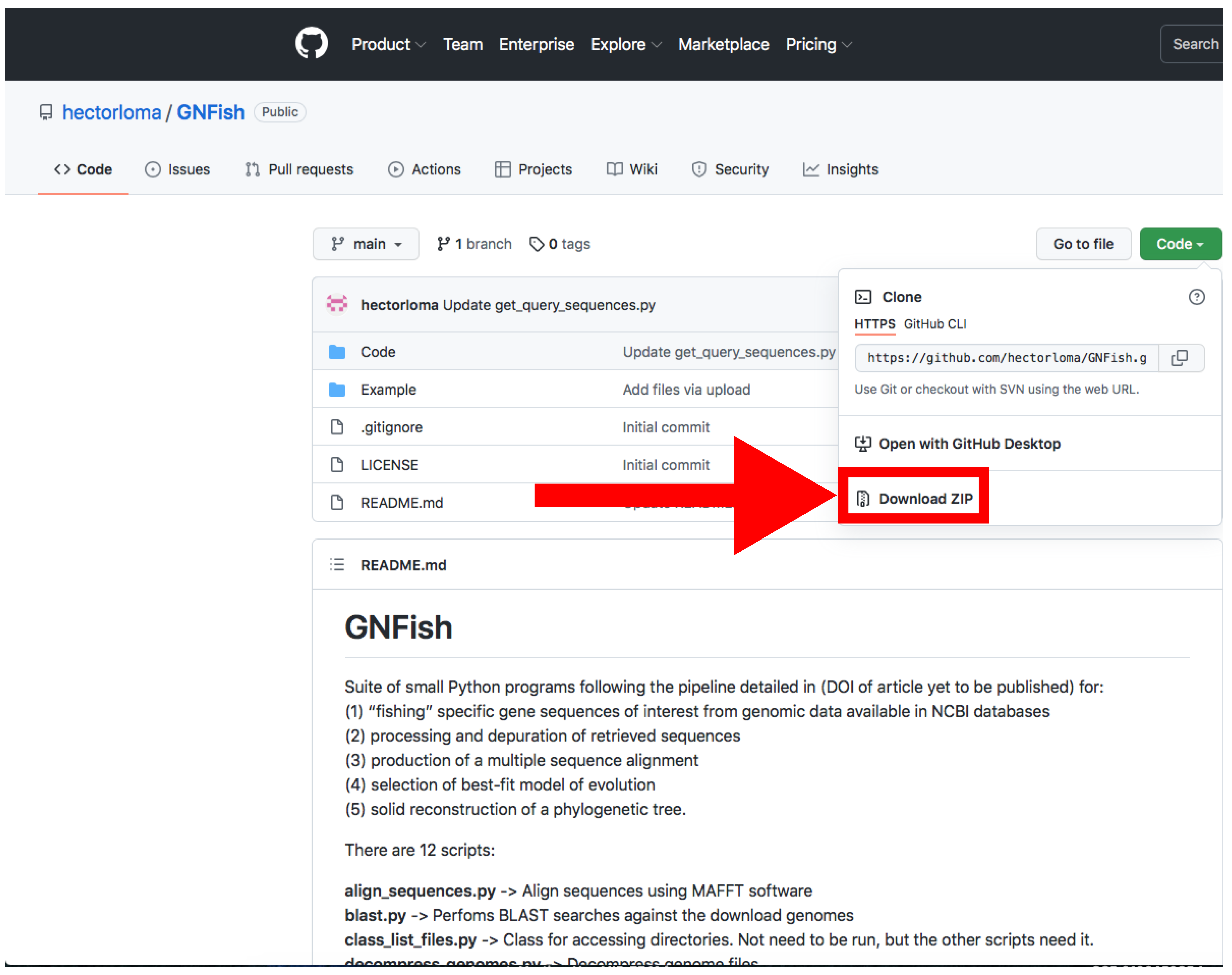
- Download the main directory containing the scripts and examples by clicking on Code → Download Zip and decompress the file (Figure 2).
- Install Anaconda following the instructions at (https://conda.io/projects/conda/en/latest/user-guide/install/index.html, accessed on 27 January 2022) and open the Spyder program.
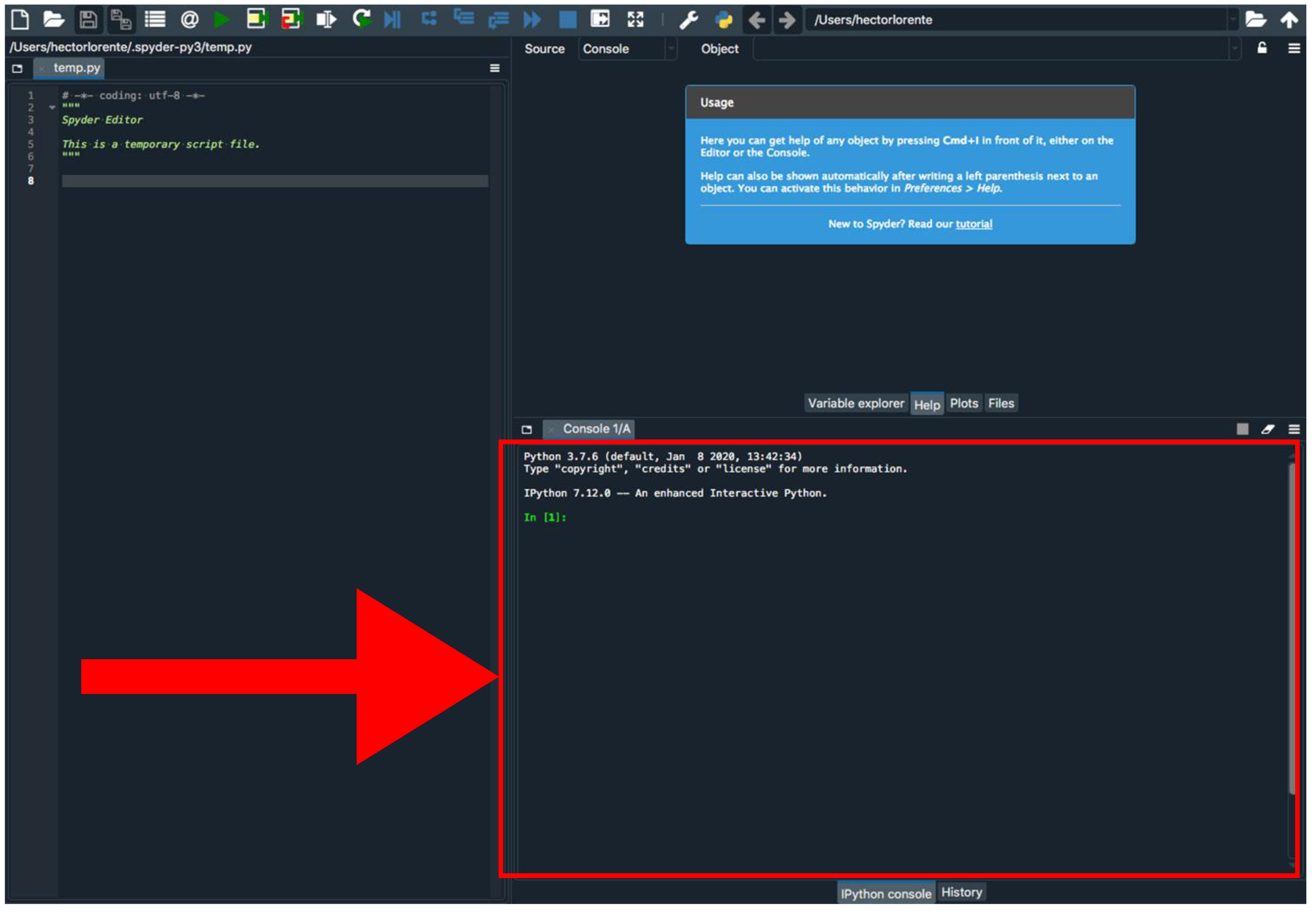
- Install Biophyton (if not installed yet). In the Spyder console (Figure 3), type pip install biopython.
- Again, in the Spyder console, type cd and drag GNFish/Code directory (remove quotes if you are a Windows user). Note that this step is mandatory every time you close the Spyder program.
- Type run get_genomes.py -h in the Spyder console to display help information and read the “README.md” file for further information and some running examples. This applies to all the “.py” programs used throughout this pipeline.
- Create a file with all your queries (usually species or higher taxon names). You can also add specific field tags (e.g., organism, assembly level, etc.) and some filters (e.g., latest [filter] or unambiguous [filter]).
- More information about how to concatenate specific field tags is found at https://www.ncbi.nlm.nih.gov/books/NBK3837/-EntrezHelp.Entrez_Searching_Options, accessed on 27 January 2022.
- For information about filters, check out https://www.ncbi.nlm.nih.gov/assembly/help/, accessed on 27 January 2022.
- For both filters and field tags, you can obtain more information after conducting a manual search. We recommend first trying a simple query with one taxa as an example following Section 3.1.1 B.
- Run the program typing run get_genomes.py [e-mail address] [path to query file] [data-type] on the Spyder console. Add any optional arguments after these mandatory ones.
- We recommend that you to use the --refine argument in order to refine your search. By default, this will apply Latest, Representative, Not Anomalous but you can add your own settings by typing them, enclosed by quotes, after the argument.
- Use the proper arguments according to your search. By default, the program will download whole-genome data. If downloading protein or RNA data, and they are not available, the program will try with the whole genome version. Stop that feature using --exclusive argument.
- Downloaded sequences will be stored into Genomic, RNA and Protein directories located at GNFish/Code/Data. Information about the downloaded genomes will be stored at Data/downloaded_genomes_log.tsv as well.
- B.
- Through NCBI Website
- Go to https://www.ncbi.nlm.nih.gov/assembly/?term=, accessed on 27 January 2022.
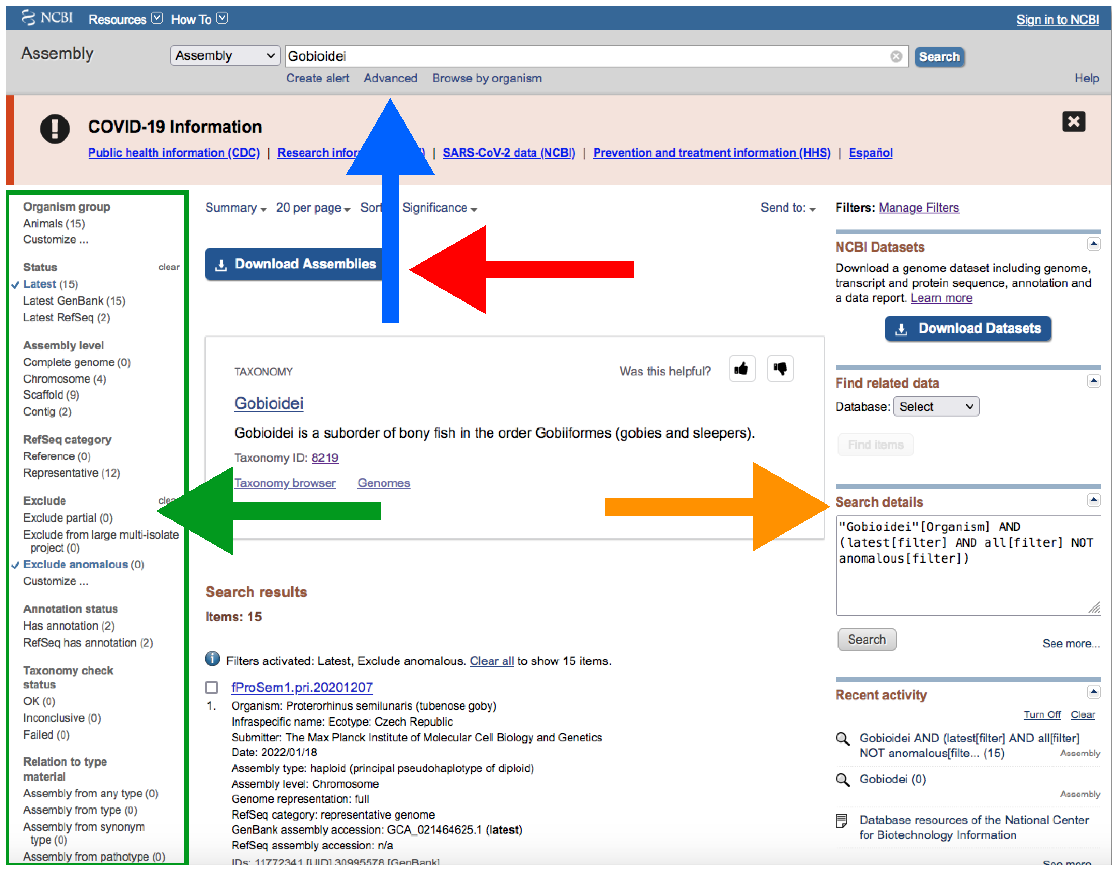
- Type your query (usually species or higher taxon names) on the search box located at the top of the web page (Figure 4).
- By clicking the Advance button right below the search box (Figure 4), you can manually add field tags (e.g., organism, assembly level, etc.).
- After your search, you would find a side bar on the left with all the available filters (Figure 4).
- In addition, you can find a text box named “Search details” on the right with the specific command of your query (Figure 4).
- This text box can be useful for creating custom queries that can be used in the automatic path (See Section 3.1.1 A).
- Note that when there are more than one field tag or filter, they appear enclosed in parentheses (Figure 4).
- We recommend keeping the default filters and adding Representative or Reference from RefSeq category by clicking on the left side panel (Figure 4) or by typing AND representative genome [filter] OR reference genome [filter] within the filter parentheses in the search box.
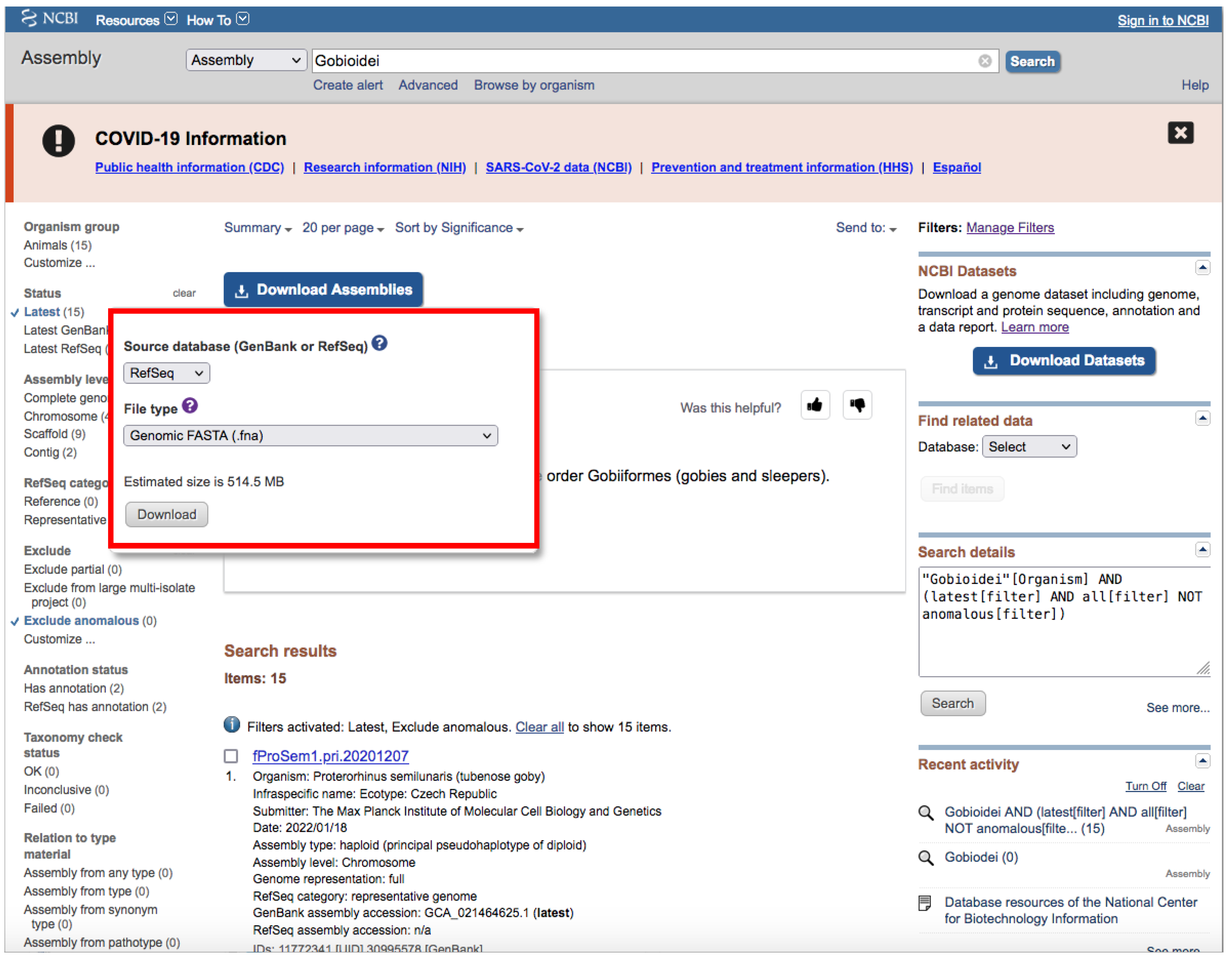
- Click on the Download Assemblies button to download the assembly (Figure 5).
- As mentioned above, genome assembly may not be evenly distributed. This can be a problem when downloading.
- We recommend that you to choose RefSeq under “Source database” (Figure 5) and either Protein FASTA (.faa) or RNA FASTA (.fna) under “File type”.
- After decompressing the downloaded file, you will find a directory tree similar to genome_assemblies_genome_fasta/ncbi-genomes-date. Within this, you will find all the files for every species.
- Then, repeat the search, but this time, when downloading, choose GenBank under “Source database” (Figure 5) and Genomic FASTA (.faa) under “File type”. Right after that, check what species were previously downloaded, and then check just the boxes of the remaining species.
- Of course, these steps are not intended for downloading a large number of genomes; for such purposes, we recommend following Section 3.1.1 A.
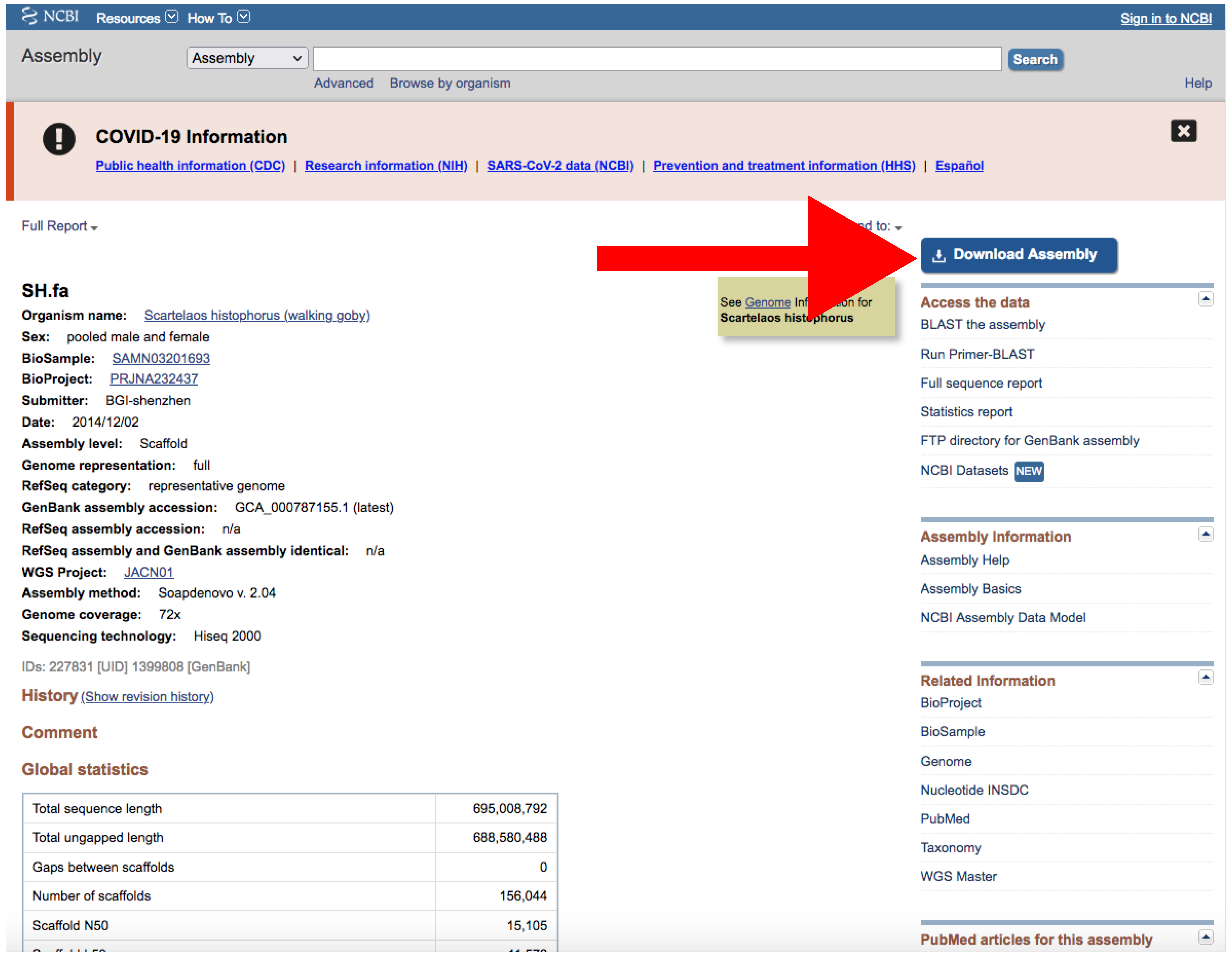
- If there is just one assembly for the selected taxa, you do not need to apply any filter. The web will automatically redirect you to the assembly entry page (Figure 6).
- We recommend storing every “.gz” file in a separate folder according to its data type (Genomic, RNA, Protein) first and then according to the species/organism.
- Download the file by clicking on Download Assemblies (Figure 6) as detailed above.
3.1.2. Generation of Query Sequences
- A.
- Locally Using Python
- Type run get_query_sequences.py [email address] [path to query file] --curated --refine. This will download a protein dataset containing 200 sequences that includes the name in “Protein Feature” (curated parameter) from “RefSeq” (refine parameter).
- The “query.txt” file can include several queries. The programs expect a gene name, with fields and filters enclosed in parentheses right after it.
- You can type your own field tags and filters, typing them after --refine argument in a similar way as when downloading genomes (See Section 3.1.1).
- In addition, you can restrict the number of downloaded sequences to a maximum number using --retmax arguments. When using --curated arguments, the program should curate sequences based upon this number; therefore, you may obtain a smaller number of sequences than with --retmax.
- There is not a perfect number of query sequences. Ideally, the best number should maximize the diversity of the studied gene family and minimize computing time. Our approach (200) aims for a great coverage of this diversity.
- BLAST can perform well with just a few sequences (around 10), reducing computing time. Therefore, another strategy could be to manually select some key sequences and download them one at a time. Of course, this requires a solid knowledge of the studied gene family.
- All this is for protein downloading, recommend as query when using BLAST searches. However, download of nucleotide sequences is also allowed (if needed for alignment; see below). However, this is not refined, so we recommend using biomol_mrna[PROP] to download just the transcripts.
- The database will be stored at Data/Query_seqs, and its name will be the name of the gene you entered, followed by “query_sequences_data_type.fas”.
- B.
- Through NCBI Website
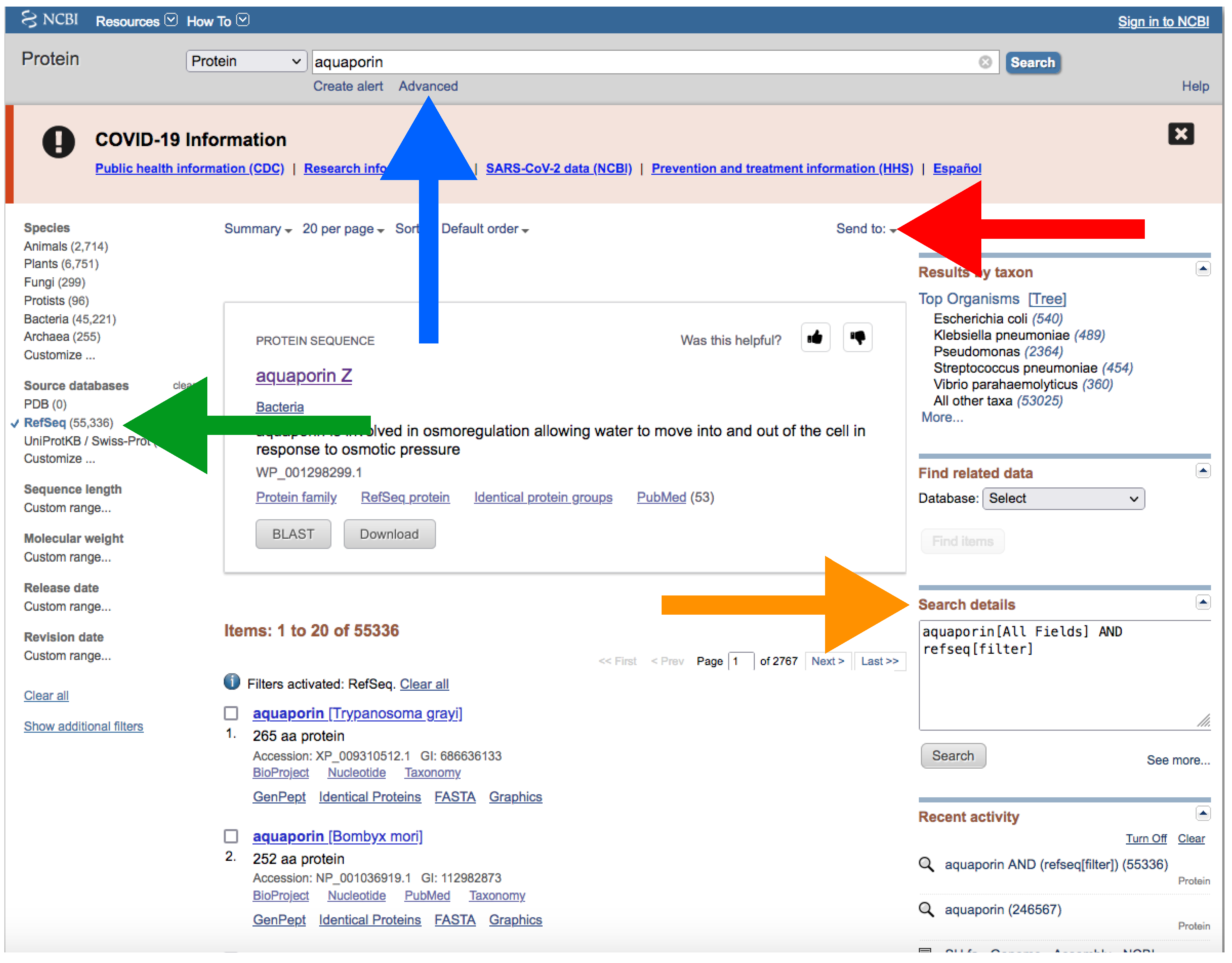
- Go to https://www.ncbi.nlm.nih.gov/protein/?term=, accessed on 27 January 2022, (Figure 7).
- Type the name of your protein in the search box at the top (Figure 7).
- In a similar way as explained for downloading genomes (see above), you can manually add field tags by clicking the Advance button right below the search box (Figure 7). You can also add filters to refine your search.
- Note that this will download the whole list of results. Therefore, it is important to be as precise as possible with your query.
- You can download nucleotide sequences in a similar way at https://www.ncbi.nlm.nih.gov/nuccocre/?term=, accessed on 27 January 2022. Type biomol_mrna[PROP] after your query to download transcripts.
3.1.3. BLAST Searches
- A.
- Locally Using Python
- Type run decompress_genomes.py in the Spyder Python console to decompress the genomic data files. Use genomic, RNA, or protein arguments or directory for your own custom path.
- Go to https://ftp.ncbi.nlm.nih.gov/blast/executables/blast+/LATEST/ (accessed on 27 January 2022) and download ncbi-blast-version-x64-win64.tar.gz (Windows users) or ncbi-blast-version-x64-linux.tar.gz (Linux and Mac users).
- Decompress the BLAST program.
- Run blast.py [blast_directory] [data_type].
- BLAST programs are located in the bin folder inside the BLAST directory. Drag the bin folder to the Spyder console after --blast_path parameter when running.
- The program will check in Genomic, RNA, and Protein directories automatically. You can change the directory by using --directory arguments, but you must also specify the genomic data type.
- You can modify the e-value parameter (see https://www.ncbi.nlm.nih.gov/books/NBK279690/, accessed on 27 January 2022, and https://www.ncbi.nlm.nih.gov/books/NBK279684/table/appendices.T.options_common_to_all_blast/ for more information, accessed on 27 January 2022). You will obtain a “.tsv” file with all the hits found in your target genomic data.
3.1.4. Extraction of RAW Sequences
- A.
- Locally Using Python
- Type run get_unique_hits.py to obtain the best hit for every of the entries of your target data.
- For whole-genome data, go to Section 3.1.4. Multiple Gene Inspection below and then continue with the next step.
- Type run get_RAW_sequences.py [data_type] to extract every sequence corresponding to each unique hit. The extracted sequences will be stored in the Extraction directory located in the same folder as the whole genome file.
- Change directory using --directory argument but keep using genomic data type.
- If using whole genome sequences, you may have to modify the --in_len parameter to control the intron length.
- Using --query_seqs arguments and typing your database file path allows you to attach some of the database sequences that match your query entry.
- By default, the program will attach the five (arbitrary number) first non-redundant sequences according to the entries of the BLAST output file. Change this using --query_seqs_num parameter.
- Note that for whole genome entries that include more than one gene, this number depends on the number of modified query entry IDs (see above).
- You can manually add any sequence. Preferably, add sequences from closely related species. You can download single sequences in the same way as the query dataset (see Section 3.1.2).
- B.
- Locally Using a Text Editor
- For whole-genome data go to Section 3.1.4. Multiple Gene Inspection below and then continue with the next step.
- Open every “whole_genome_name_out.tsv” file. Look at the second column (target ID) and keep just unique IDs. For whole-genome data, follow Section 3.1.4 A.
- Open your genomic data (i.e., Genus_species_id.faa) with a text editor. This step cannot be performed in some cases, especially those that imply the use of non-annotated genome sequences.
- Pick up every unique target ID and search for it in the corresponding genomic data file.
- The following steps assume that you have used --outfmt 6 (i.e., BLAST tabular output format 6).
- Open the “whole_genome_name_out.tsv” file with a spreadsheet program (such as Microsoft Excel) or a text editor.
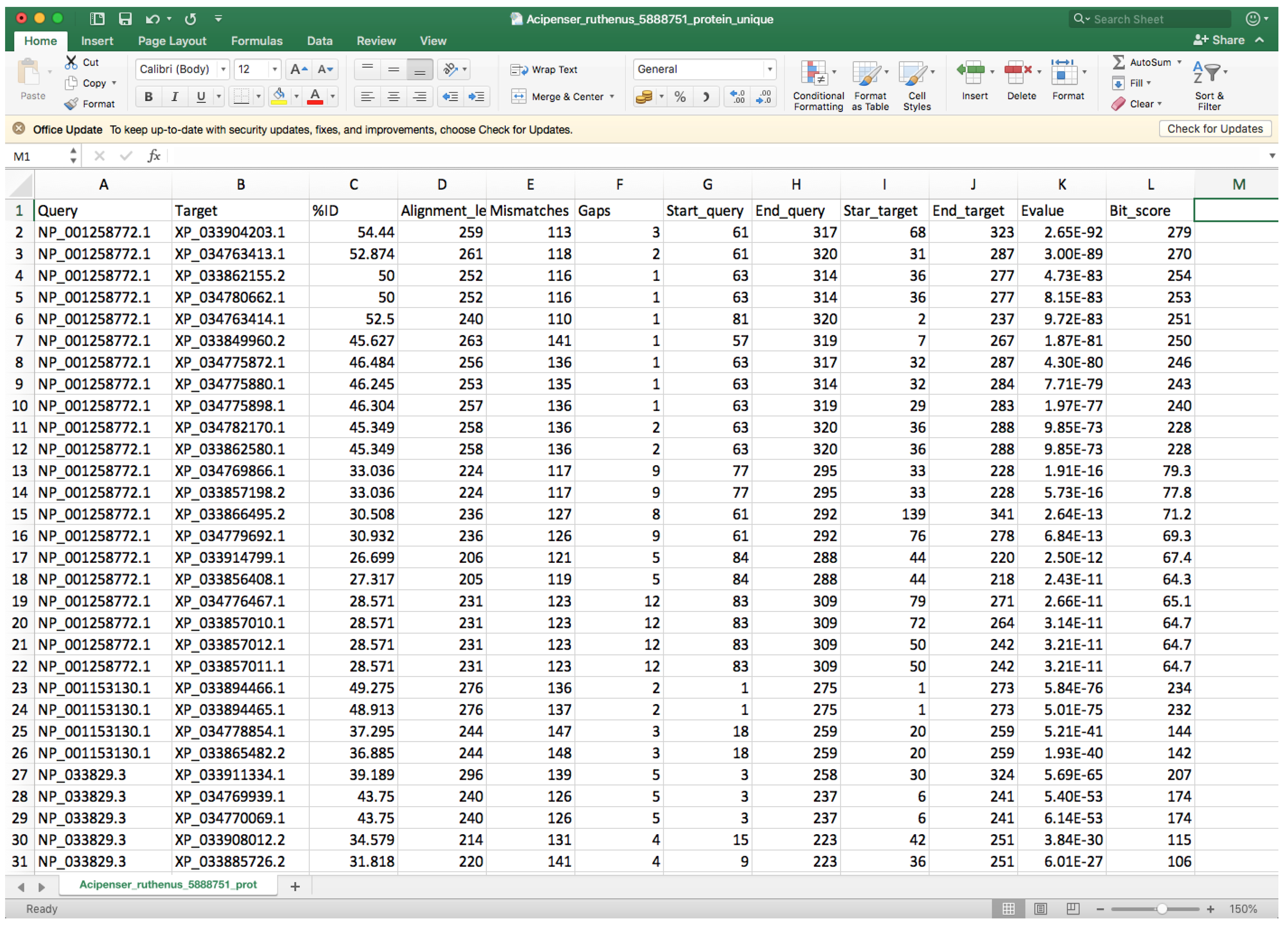
- Every row corresponds to a different hit, and the second column indicates the target identifier (scaffold ID) (Figure 8).
- Controlling by the 2nd column, you must check the 9th and 10th columns that contain the start and end positions where the query sequence aligned within the target entry and compare entries below to identify different start or end positions that could be associated with two different genes.
- In order to facilitate visibility, you can highlight every target by clicking on Conditional Formatting → Highlight Cells Rules → Equal to → Choose the corresponding cell → OK.
- You can also highlight the 9th and 10th columns in the same way using Between to instead of Equal to for controlling.
- If you spot another gene in the same query entry, you must modify the query entry ID (first column) by adding “_1” to the rows that belong to the first one, “_2” to the second one, etc. We recommend changing at least five query entry IDs if possible in order to facilitate proper gene fishing (see below). Additionally, you must update the “_unique.tsv” file with the new query names, and you must add at least one row containing the information of the new gene(s).
- Before continuing with the next target ID, click on Conditional Formatting → Clear Rules → Clear Rules for Entire set.
3.1.5. Coding Sequence Identification (Although This Step Is Mandatory When Working with Whole Genome Sequences, You Can Skip It When Working with Protein and RNA Sequences)
- You should have used --query_seqs earlier (Section 3.1.4 A) to attach template sequences or have manually added some.
Alignment
- A.
- Locally Using Python
- Go to MAFFT software web (https://mafft.cbrc.jp/alignment/software/, accessed on 27 January 2022) and navigate to the specific page according to your operating system. Follow the steps to install MAFFT software on your computer.
- On the Spyder Python console, type run align_sequences.py. You can choose a specific alignment algorithm using --algorithm. The MAFFT manual recommends using the Auto function when you know little about your data. For genomic data and working with one gene family, we recommend using the E-INS-i algorithm.
- As in other cases, you can use genomic, rna, and protein or directory arguments.
- Windows users may encounter some problems in either installing or running MAFFT, especially those using older system versions. If this is the case, look at the next section.
- B.
- Through MAFFT Server
- Go to the MAFFT online version page (https://mafft.cbrc.jp/alignment/server/, accessed on 27 January 2022).
- Paste the content of the file you want to align in the available text box or browse for your file by clicking on the Choose File button.
- Select Same as input for the options: UPPERCASE/lowercase, Direction of nucleotide sequences, and Output order.
- Scroll down to the Advance settings section. In the Strategy section, we recommend using Auto if you know little about your data. For genomic data, we recommend using the E-INS-i algorithm.
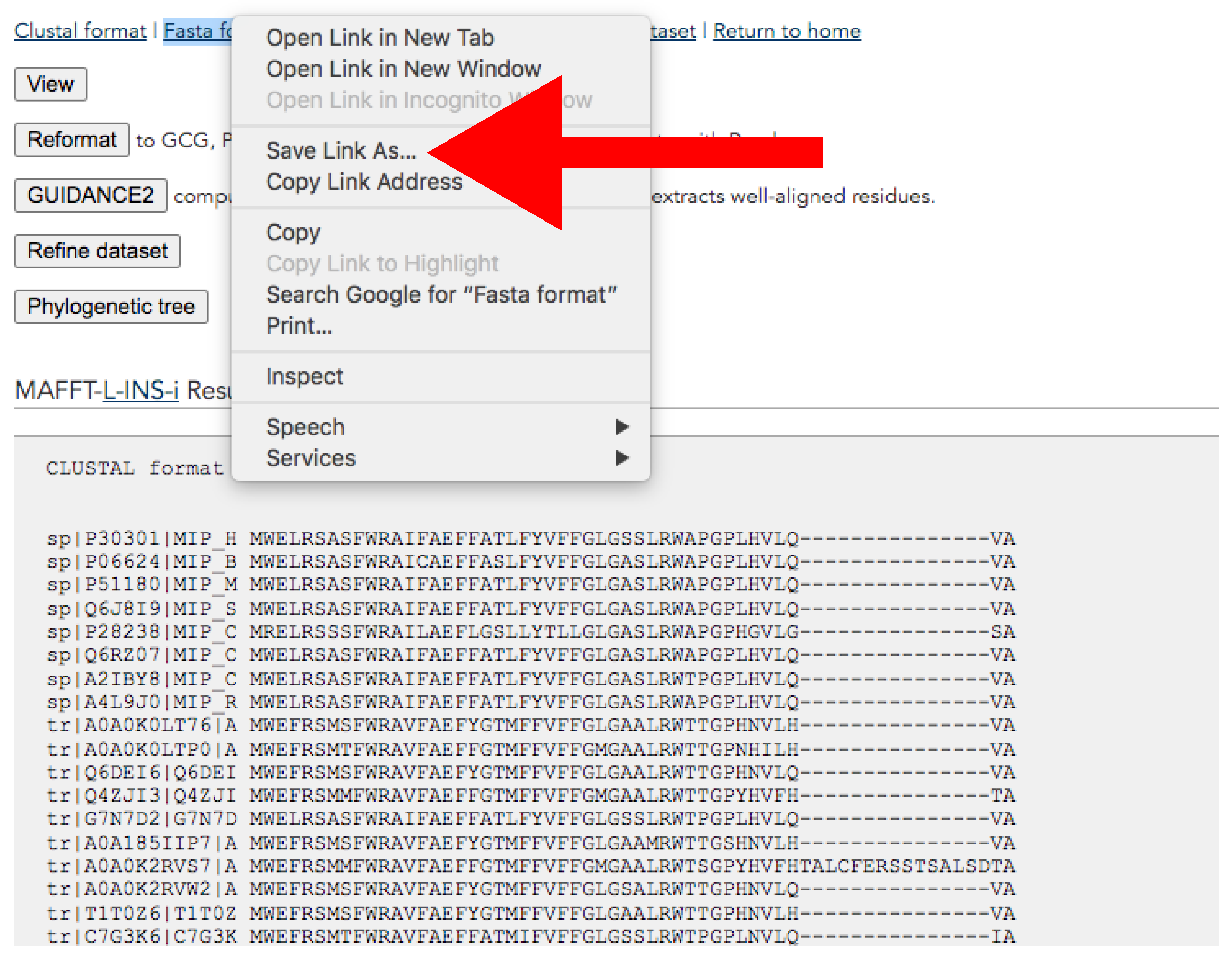
- Download the alignment from the results page (Figure 9). This page will pop up after the alignment run is completed.
- At the top of the page, click the right button of the mouse over Fasta format → Save link as → Save it adding “_final.fas” suffix (Figure 9).
Trimming and Retrieving Coding Sequences (Using MEGA Version 11)
- Go to the MEGA home page (https://www.megasoftware.net/, accessed on 27 January 2022), select your operating system, Graphical GUI, and MEGA 11 (or newer versions if available), and click on the Download button.
- Follow the steps for MEGA downloading and installation.
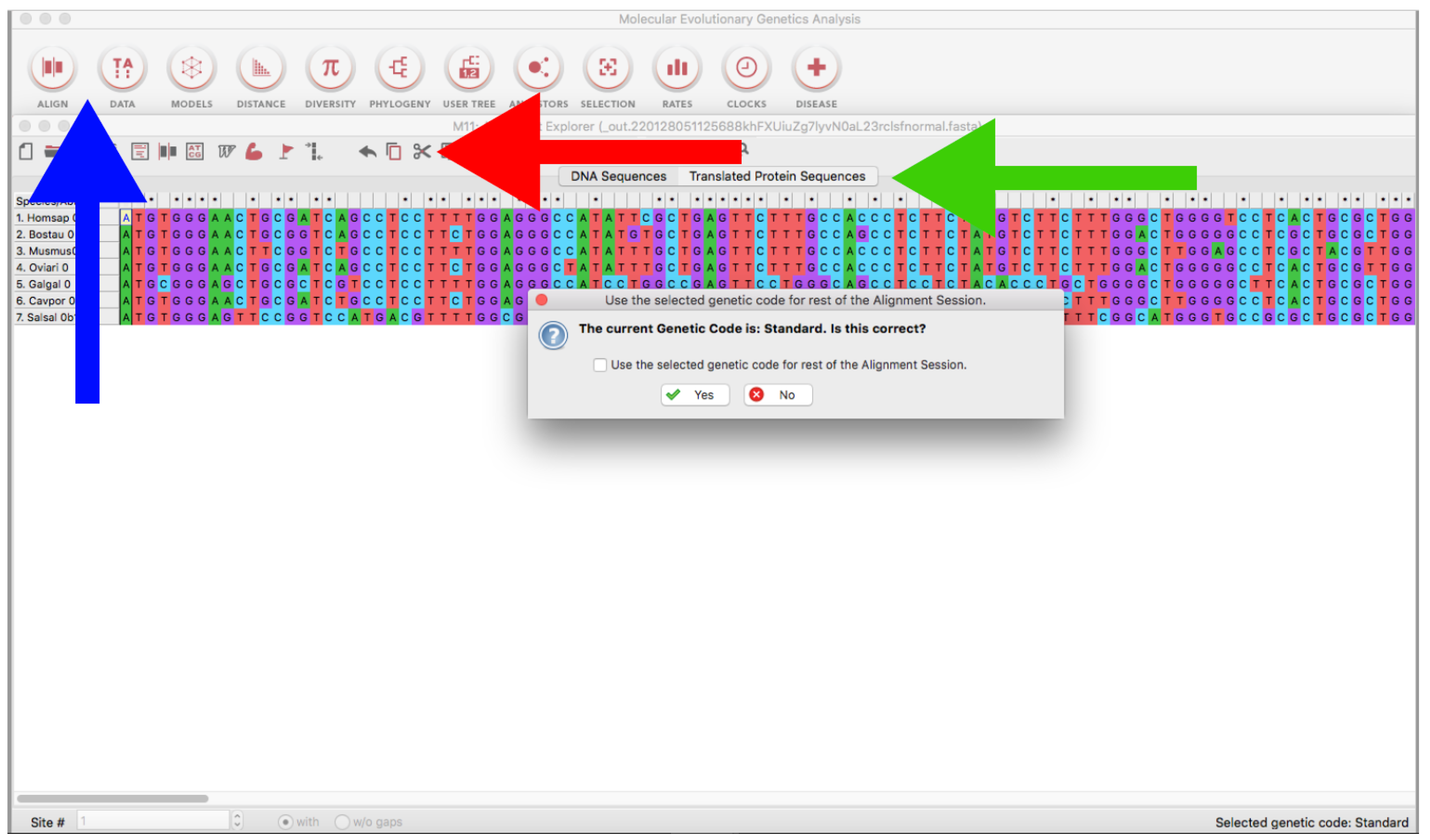
- Open the MEGA program and load every alignment file (ALIGN → Edit/Build Alignment → Open a saved alignment version → OK → Open the downloaded file) (Figure 10).
- Trim the sequences using the Scissors tool (Figure 10) or using Ctrl or Cmmd + X. If you are using genomic or RNA data, you can click on Translated Protein Sequences to obtain the deduced amino acid sequences (see also Section 3.2.1), which can be useful for delimiting open reading frames (identification of start/stop codons and intronic/exonic regions by visual inspection).
- Finally, click on Data → Export Alignment → Fasta Format → Save it.
- When working with genomic sequences, it may be necessary to conduct steps in Section 3.1.5 several times (iterative refinement) in order to eventually obtain the coding sequence of interest. The alignment becomes progressively refined by iteratively trimming intronic regions and leftover positions at the beginning and the end of the sequence.
- In some cases, you will have to rerun get_RAW_sequences.py, changing the --in_len parameter value in order to cover all the sequence. Sometimes the chosen value may be too small, and part of the sequence can be left out unintentionally.
- Once the coding sequence has been fully identified, save the alignment with MEGA as detailed above and add the suffix, “_final.fas”.
3.2. Phylogenetic Analyses
3.2.1. Translate Sequences
- A.
- Locally Using Python
- This step is mandatory if you want to obtain a protein data matrix
- and you are working with genomic or RNA sequences.
- In the Spyder console, type run translate_sequences.py [data_type]. Typically, you are going to use it with genomic sequences or, in some cases, with RNA sequences (particularly for checking and removing ambiguously aligned positions).
- By default, the program will look for files with “final.fas” or “RAW.fas”. Change this using the --pattern parameter.
- If you are working with several species that each have a different genetic code, you will have to run this program several times. We recommend cutting those folders that share the same genetic code and pasting them into a new folder. Use --directory arguments to indicate the new path and run the program. Then, put the folders back in their initial location and repeat the step with the different genetic codes.
- B.
- Locally Using MEGA
- Open the MEGA program (see Section 3.1.5. Trimming and Retrieving Coding Sequences for MEGA installation).
- Import alignment as in Section 3.1.5. Trimming and Retrieving Coding Sequences (Figure 10).
- On the emergent window, click on Translated Protein Sequences → Choose the adequate genetic code (Figure 10).
- Finally, click on Data → Export Alignment → Fasta Format → Save with “_translated.fas” suffix.
- Repeat with all the files that need to be translated.
3.2.2. Matrix Assembly
- A.
- Locally Using Python
- In the Spyder Python console, type run get_combined_seqs.py [output name][data_type]. The three data types can be combined. However, note that if you have information for more than one data type for the same species, then you may obtain redundant sequences.
- By default, the pattern for file searching is “final.fas”. However, it is programmed to look for “final_translated.fas”, “RAW.fas”, and “RAW_translated.fas” when it cannot find the first pattern.
- You can change this using the --pattern parameter. Then, the program will search for “new_pattern.fas”, “new_pattern_translated.fas”, “RAW.fas”, and “RAW_translated.fas”.
- The program will produce a data matrix named “[output name]_all_combined.fas”, which will be downloaded to the Data folder.
- B.
- Locally Using MEGA
- Import a sequence file as in Section 3.1.5. Alignment B. (Figure 10).
- In the emergent window, click on Edit → Insert Sequence From File → Open every sequence file (Figure 10).
- This step can also be conducted manually with a text editor; simply open every file containing the downloaded sequences and paste their content into a new file, one after the other.
3.2.3. Alignment
- See Section 3.1.5. Alignment. If using the Python version, use –directory, and drag the combined matrix file.
Alignment Filtering
- A.
- Using trimAl Locally through Python
- Go to http://trimal.cgenomics.org/downloads (accessed on 27 January 2022) and download the specific program according to your operating system.
- Decompress the trimAl file. For Windows and Mac/Unix users, open the terminal and follow the steps on the trimAl README.md file. You can run the program on the terminal following the instructions at http://trimal.cgenomics.org/use_of_the_command_line_trimal_v1.2 (accessed on 27 January 2022) or the following steps.
- Type run alignment_trimming.py [path_to trimAl] [path_to_matrix] [combined_matrix] in the Spyder console. For Windows users, trimAl will be stored in the bin directory. For Mac and Unix users, trimAl will be stored in the source directory.
- This will remove all positions in the alignment with gaps in 90% or more of the sequences (-gt 0.9), which is the default option of the program.
- The trimming algorithm can be changed using --trimal_command. See http://trimal.cgenomics.org/use_of_the_command_line_trimal_v1.2 (accessed on 27 January 2022) for additional information.
- B.
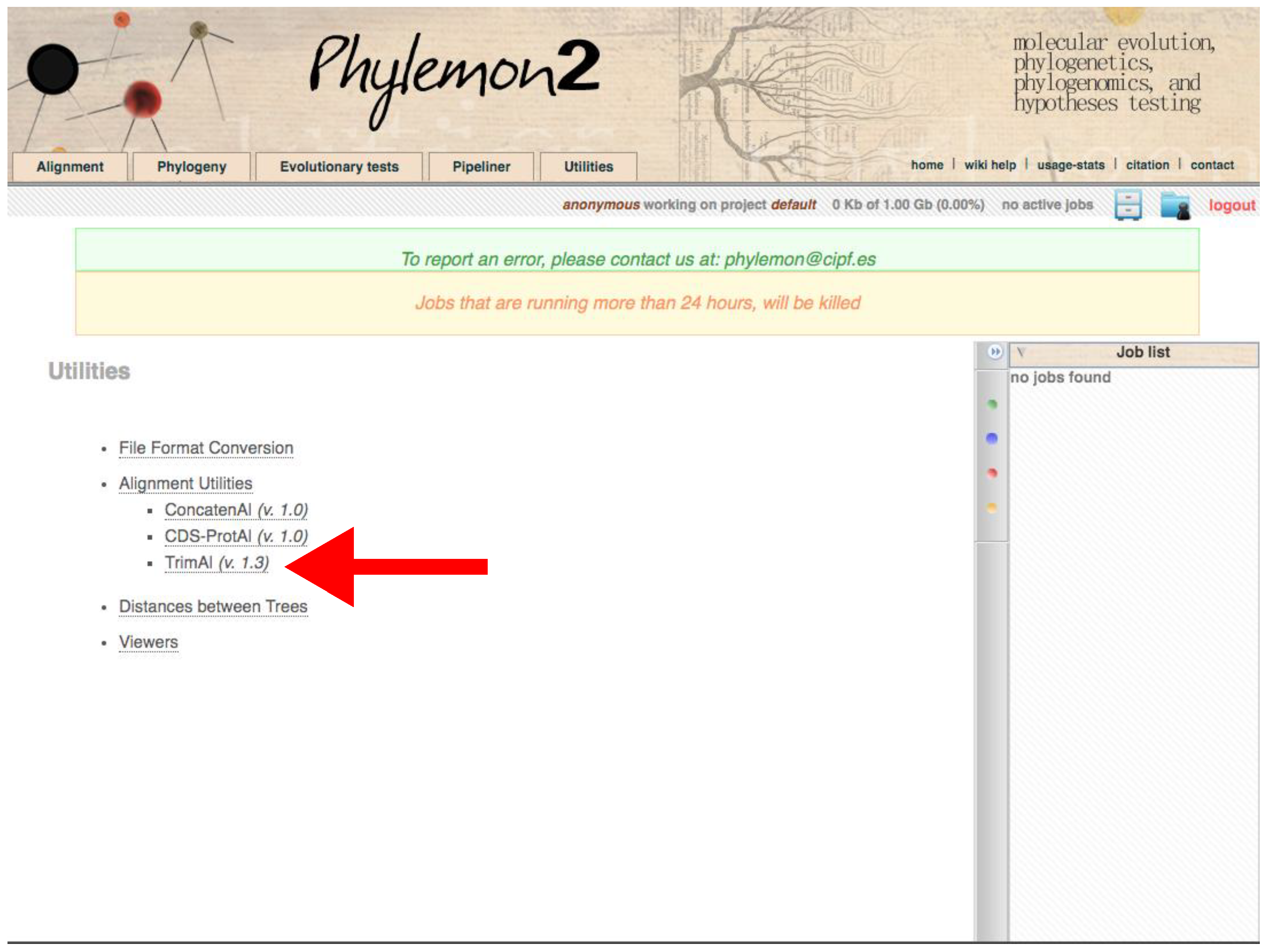
- Using trimAl through the Phylemon Web Server
- Go to http://phylemon2.bioinfo.cipf.es/, accessed on 27 January 2022.
- Create and account and login or star as anonymous user.
- Paste the content of the matrix or upload the file clicking on browse server → Upload new file → Browse → Open the matrix → Select format → Aligned sequences → Upload → Accept.
- Click on Method → User define → In Gap threshold, fraction of positions without gaps in a column set 0.1. Similar output as using Python version.
- Run the job.
- Refresh the page. On the right panel, open the job when finished.
3.2.4. Phylogeny Inference
- A.
- Using IQ-TREE Locally through Python
- Go to http://www.iqtree.org/#download (accessed on 27 January 2022) and download the adequate version for your operating system.
- Decompress the folder.
- Type run phylogenetic_inference.py [iqtree_folder] [trimmed_matrix] [data_type].
- IQ-TREE program is located in the bin folder in the IQ-TREE program folder. Drag this folder to the Spyder console when running.
- The “.treefile” will be stored at Data/Phylogenetic_inference.
- B.
- Using IQ-TREE Web Server
- Go to http://iqtree.cibiv.univie.ac.at/, accessed on 27 January 2022.
- Browse the trimmed matrix in the Alignment file field.
- Select sequence type.
- Do not change any more parameters for a similar run and output as the Python version.
- Enter your e-mail and click on SUBMIT JOB.
- When finished, you will receive and e-mail. Click on the provided link, and with the button on the left, click DOWNLOAD SELECTED JOBS.
Tree Visualization
- Go to the FigTree website (https://github.com/rambaut/figtree/releases (accessed on 27 January 2022)) and download the specific version for your operating system.
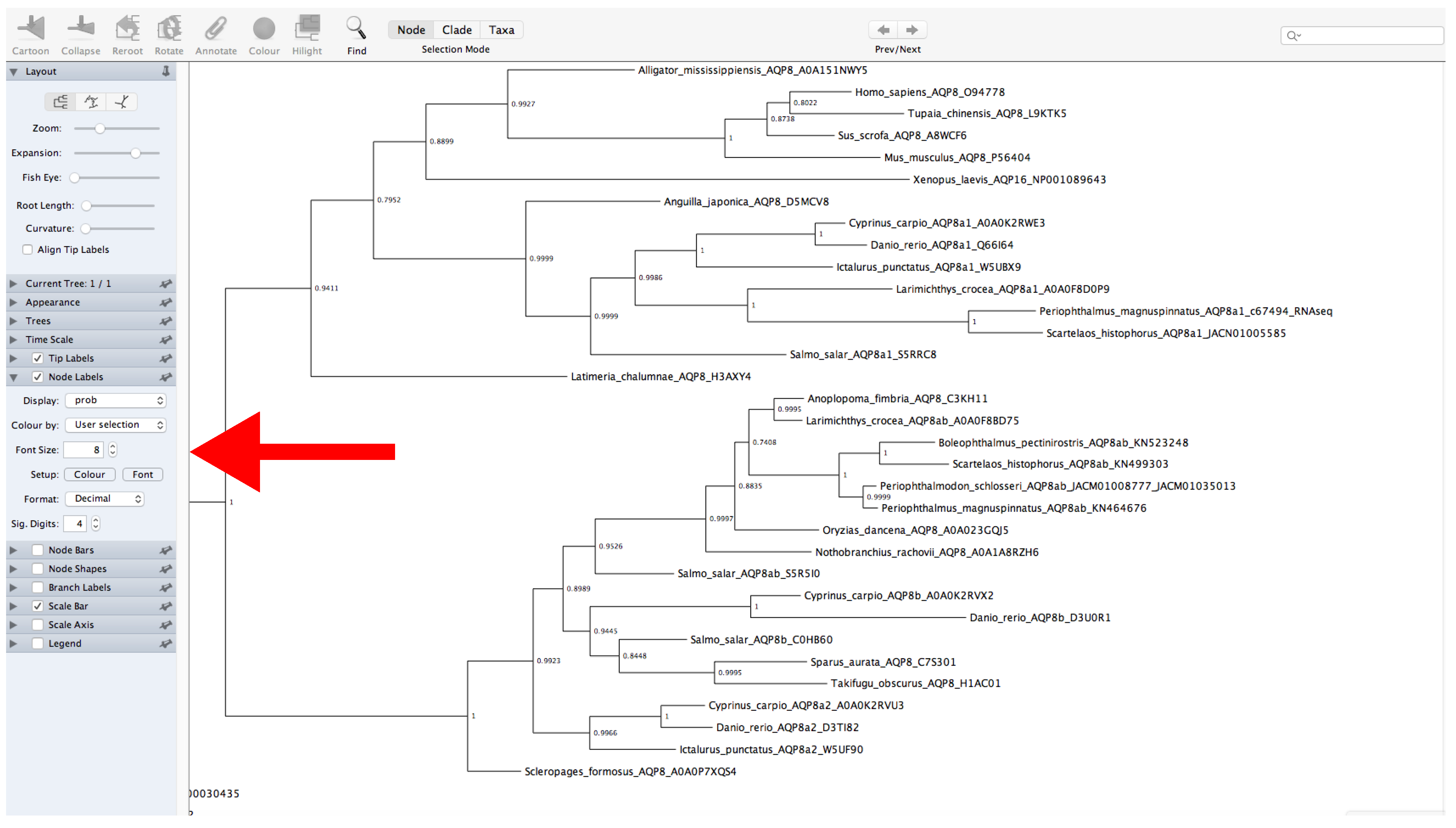
- Decompress the file and open FigTree (Figure 12).
- Click on File → Open → Open “.treefile” file.
- Provide a label for the values of support (or leave unchanged).
- The left panel allows for modification of multiple tree features displayed as collapsible menus. For example, tree appearance options can be changed from the Appearance menu.
- Display the values of support. Click on Node Labels → Display → Select the name of the label provided before (Figure 12).
- The root of the tree can be changed by selecting a specific branch and then clicking the Reroot button at the top of the window.
4. Expected Results
5. Troubleshooting
Author Contributions
Funding
Institutional Review Board Statement
Informed Consent Statement
Data Availability Statement
Acknowledgments
Conflicts of Interest
References
- Ekblom, R.; Galindo, J. Applications of next generation sequencing in molecular ecology of non-model organisms. Heredity 2011, 107, 1–15. [Google Scholar] [CrossRef] [PubMed] [Green Version]
- Lee, C.Y.; Chiu, Y.C.; Wang, L.B.; Kuo, Y.L.; Chuang, E.Y.; Lai, L.C.; Tsai, M.H. Common applications of next-generation sequencing technologies in genomic research. Transl. Cancer Res. 2013, 2, 33–45. [Google Scholar] [CrossRef]
- Shendure, J.; Ji, H. Next-generation DNA sequencing. Nat. Biotechnol. 2008, 26, 1135–1145. [Google Scholar] [CrossRef] [PubMed]
- Schadt, E.E.; Turner, S.; Kasarskis, A. A window into third-generation sequencing. Hum. Mol. Genet. 2010, 19, R227–R240. [Google Scholar] [CrossRef]
- Hardison, R.C. Comparative Genomics. PLoS Biol. 2003, 1, e58. [Google Scholar] [CrossRef]
- San Mauro, D.; Agorreta, A. Molecular systematics: A synthesis of the common methods and the state of knowledge. Cell. Mol. Biol. Lett. 2010, 15, 311–341. [Google Scholar] [CrossRef] [Green Version]
- Alioto, T.; Blanco, E.; Parra, G.; Guigó, R. Using geneid to Identify Genes. Curr. Protoc. Bioinform. 2018, 64, e56. [Google Scholar] [CrossRef]
- Seemann, T. Prokka: Rapid prokaryotic genome annotation. Bioinformatics 2014, 30, 2068–2069. [Google Scholar] [CrossRef]
- Brůna, T.; Lomsadze, A.; Borodovsky, M. GeneMark-EP+: Eukaryotic gene prediction with self-training in the space of genes and proteins. NAR Genom. Bioinform. 2020, 2, lqaa026. [Google Scholar] [CrossRef]
- Kornobis, E.; Cabellos, L.; Aguilar, F.; Frías-López, C.; Rozas, J.; Marco, J.; Zardoya, R. TRUFA: A user-friendly web server for de novo rna-seq analysis using cluster computing. Evol. Bioinform. 2015, 11, EBO-S23873. [Google Scholar] [CrossRef] [Green Version]
- Wheeler, D.; Bhagwat, M. BLAST QuickStart: Example-driven web-based BLAST tutorial. Methods Mol. Biol. 2007, 395, 149–176. [Google Scholar] [CrossRef] [PubMed]
- Inoue, J.; Satoh, N. ORTHOSCOPE: An Automatic Web Tool for Phylogenetically Inferring Bilaterian Orthogroups with User-Selected Taxa. Mol. Biol. Evol. 2019, 36, 621–631. [Google Scholar] [CrossRef] [PubMed]
- Cock, P.J.A.; Antao, T.; Chang, J.T.; Chapman, B.A.; Cox, C.J.; Dalke, A.; Friedberg, I.; Hamelryck, T.; Kauff, F.; Wilczynski, B.; et al. Biopython: Freely available Python tools for computational molecular biology and bioinformatics. Bioinformatics 2009, 25, 1422–1423. [Google Scholar] [CrossRef] [PubMed]
- Richter, D.J.; Berney, C.; Strassert, J.F.H.; Burki, F.; de Vargas, C. EukProt: A database of genome-scale predicted proteins across the diversity of eukaryotic life. bioRxiv 2020. [Google Scholar] [CrossRef]
- Howe, K.L.; Achuthan, P.; Allen, J.; Allen, J.; Alvarez-Jarreta, J.; Ridwan Amode, M.; Armean, I.M.; Azov, A.G.; Bennett, R.; Bhai, J.; et al. Ensembl 2021. Nucleic Acids Res. 2021, 49, D884–D891. [Google Scholar] [CrossRef]
- Sayers, E.W.; Beck, J.; Bolton, E.E.; Bourexis, D.; Brister, J.R.; Canese, K.; Comeau, D.C.; Funk, K.; Kim, S.; Klimke, W.; et al. Database resources of the National Center for Biotechnology Information. Nucleic Acids Res. 2021, 49, D10–D17. [Google Scholar] [CrossRef]
- Pruitt, K.D.; Tatusova, T.; Maglott, D.R. NCBI reference sequences (RefSeq): A curated non-redundant sequence database of genomes, transcripts and proteins. Nucleic Acids Res. 2007, 35, D61–D65. [Google Scholar] [CrossRef] [Green Version]
- Schuler, G.D.; Epstein, J.A.; Ohkawa, H.; Kans, J.A. [10] Entrez: Molecular biology database and retrieval system. Methods Enzymol. 1996, 266, 141–162. [Google Scholar] [CrossRef]
- Altschul, S.F.; Gish, W.; Miller, W.; Myers, E.W.; Lipman, D.J. Basic local alignment search tool. J. Mol. Biol. 1990, 215, 403–410. [Google Scholar] [CrossRef]
- Notredame, C. Recent evolutions of multiple sequence alignment algorithms. PLoS Comput. Biol. 2007, 3, e123. [Google Scholar] [CrossRef] [Green Version]
- Katoh, K.; Rozewicki, J.; Yamada, K.D. MAFFT online service: Multiple sequence alignment, interactive sequence choice and visualization. Brief. Bioinform. 2019, 20, 1160–1166. [Google Scholar] [CrossRef] [PubMed] [Green Version]
- Katoh, K.; Misawa, K.; Kuma, K.I.; Miyata, T. MAFFT: A novel method for rapid multiple sequence alignment based on fast Fourier transform. Nucleic Acids Res. 2002, 30, 3059–3066. [Google Scholar] [CrossRef] [PubMed] [Green Version]
- Thompson, J.D.; Gibson, T.J.; Higgins, D.G. Multiple Sequence Alignment Using ClustalW and ClustalX. Curr. Protoc. Bioinform. 2003, 1, 2.3.1–2.3.22. [Google Scholar] [CrossRef] [PubMed]
- Di Tommaso, P.; Moretti, S.; Xenarios, I.; Orobitg, M.; Montanyola, A.; Chang, J.M.; Taly, J.F.; Notredame, C. T-Coffee: A web server for the multiple sequence alignment of protein and RNA sequences using structural information and homology extension. Nucleic Acids Res. 2011, 39, W13–W17. [Google Scholar] [CrossRef]
- Tamura, K.; Stecher, G.; Kumar, S. MEGA11: Molecular Evolutionary Genetics Analysis Version 11. Mol. Biol. Evol. 2021, 38, 3022–3027. [Google Scholar] [CrossRef]
- Phillips, A.; Janies, D.; Wheeler, W. Multiple sequence alignment in phylogenetic analysis. Mol. Phylogenet. Evol. 2000, 16, 317–330. [Google Scholar] [CrossRef]
- Goldman, N. Effects of sequence alignment procedures on estimates of phylogeny. BioEssays 1998, 20, 287–290. [Google Scholar] [CrossRef]
- Ogden, T.H.; Rosenberg, M.S. Multiple sequence alignment accuracy and phylogenetic inference. Syst. Biol. 2006, 55, 314–328. [Google Scholar] [CrossRef] [Green Version]
- Talavera, G.; Castresana, J. Improvement of phylogenies after removing divergent and ambiguously aligned blocks from protein sequence alignments. Syst. Biol. 2007, 56, 564–577. [Google Scholar] [CrossRef] [PubMed] [Green Version]
- Capella-Gutiérrez, S.; Silla-Martínez, J.M.; Gabaldón, T. trimAl: A tool for automated alignment trimming in large-scale phylogenetic analyses. Bioinformatics 2009, 25, 1972–1973. [Google Scholar] [CrossRef]
- Sánchez, R.; Serra, F.; Tárraga, J.; Medina, I.; Carbonell, J.; Pulido, L.; De María, A.; Capella-Gutíerrez, S.; Huerta-Cepas, J.; Gabaldón, T.; et al. Phylemon 2.0: A suite of web-tools for molecular evolution, phylogenetics, phylogenomics and hypotheses testing. Nucleic Acids Res. 2011, 39, W470–W474. [Google Scholar] [CrossRef] [Green Version]
- Cunningham, C.W.; Zhu, H.; Hillis, D.M. Best-fit maximum-likelihood models for phylogenetic inference: Empirical tests with known phylogenies. Evolution 1998, 52, 978–987. [Google Scholar] [CrossRef] [PubMed]
- Bruno, W.J.; Halpern, A.L. Topological bias and inconsistency of maximum likelihood using wrong models. Mol. Biol. Evol. 1999, 16, 564–566. [Google Scholar] [CrossRef] [PubMed] [Green Version]
- Huelsenbeck, J.P.; Hillis, D.M. Success of phylogenetic methods in the four taxon case. Syst. Biol. 1993, 42, 247–264. [Google Scholar] [CrossRef]
- Nguyen, L.T.; Schmidt, H.A.; Von Haeseler, A.; Minh, B.Q. IQ-TREE: A fast and effective stochastic algorithm for estimating maximum-likelihood phylogenies. Mol. Biol. Evol. 2015, 32, 268–274. [Google Scholar] [CrossRef]
- Minh, B.Q.; Nguyen, M.A.T.; Von Haeseler, A. Ultrafast approximation for phylogenetic bootstrap. Mol. Biol. Evol. 2013, 30, 1188–1195. [Google Scholar] [CrossRef]
- Yang, Z. Maximum-likelihood estimation of phylogeny from DNA sequences when substitution rates differ over sites. Mol. Biol. Evol. 1993, 10, 1188–1195. [Google Scholar] [CrossRef] [Green Version]
- Koshi, J.M.; Goldstein, R.A. Context-dependent optimal substitution matrices. Protein Eng. Des. Sel. 1995, 8, 641–645. [Google Scholar] [CrossRef]
- Goldman, N.; Thorne, J.L.; Jones, D.T. Assessing the impact of secondary structure and solvent accessibility on protein evolution. Genetics 1998, 149, 445–458. [Google Scholar] [CrossRef]
- Thorne, J.L.; Goldman, N.; Jones, D.T. Combining protein evolution and secondary structure. Mol. Biol. Evol. 1996, 13, 666–673. [Google Scholar] [CrossRef] [Green Version]
- Le, S.Q.; Lartillot, N.; Gascuel, O. Phylogenetic mixture models for proteins. Philos. Trans. R. Soc. B Biol. Sci. 2008, 363, 3965–3976. [Google Scholar] [CrossRef] [PubMed] [Green Version]
- Bateman, A. UniProt: A worldwide hub of protein knowledge. Nucleic Acids Res. 2019, 47, D506–D515. [Google Scholar] [CrossRef] [Green Version]
- Finn, R.D.; Clements, J.; Eddy, S.R. HMMER web server: Interactive sequence similarity searching. Nucleic Acids Res. 2011, 39, W29–W37. [Google Scholar] [CrossRef] [PubMed] [Green Version]
- El-Gebali, S.; Mistry, J.; Bateman, A.; Eddy, S.R.; Luciani, A.; Potter, S.C.; Qureshi, M.; Richardson, L.J.; Salazar, G.A.; Smart, A.; et al. The Pfam protein families database in 2019. Nucleic Acids Res. 2019, 47, D427–D432. [Google Scholar] [CrossRef]
- Hunter, S.; Apweiler, R.; Attwood, T.K.; Bairoch, A.; Bateman, A.; Binns, D.; Bork, P.; Das, U.; Daugherty, L.; Duquenne, L.; et al. InterPro: The integrative protein signature database. Nucleic Acids Res. 2009, 37, D211–D215. [Google Scholar] [CrossRef] [Green Version]
- Löytynoja, A. Phylogeny-aware alignment with PRANK. In Multiple Sequence Alignment Methods; Russell, D.J., Ed.; Humana Press: Totowa, NJ, USA, 2014; pp. 155–170. [Google Scholar] [CrossRef]
- Guindon, S.; Lethiec, F.; Duroux, P.; Gascuel, O. PHYML Online—A web server for fast maximum likelihood-based phylogenetic inference. Nucleic Acids Res. 2005, 33, W557–W559. [Google Scholar] [CrossRef] [Green Version]
- Stamatakis, A. RAxML version 8: A tool for phylogenetic analysis and post-analysis of large phylogenies. Bioinformatics 2014, 30, 1312–1313. [Google Scholar] [CrossRef]
- Darriba, D.; Taboada, G.L.; Doallo, R.; Posada, D. ProtTest 3: Fast selection of best-fit models of protein evolution. Bioinformatics 2011, 27, 1164–1165. [Google Scholar] [CrossRef] [Green Version]
- Darriba, D.; Taboada, G.L.; Doallo, R.; Posada, D. JModelTest 2: More models, new heuristics and parallel computing. Nat. Methods 2012, 9, 1164–1165. [Google Scholar] [CrossRef] [Green Version]
- Lanfear, R.; Calcott, B.; Ho, S.Y.W.; Guindon, S. PartitionFinder: Combined selection of partitioning schemes and substitution models for phylogenetic analyses. Mol. Biol. Evol. 2012, 29, 1695–1701. [Google Scholar] [CrossRef] [Green Version]
- Rambaut, A. FigTree v1.4.4. Available online: http://tree.bio.ed.ac.uk/software/figtree/ (accessed on 27 January 2022).
- Huson, D.H.; Scornavacca, C. Dendroscope 3: An interactive tool for rooted phylogenetic trees and networks. Syst. Biol. 2012, 61, 1061–1067. [Google Scholar] [CrossRef] [PubMed] [Green Version]

Publisher’s Note: MDPI stays neutral with regard to jurisdictional claims in published maps and institutional affiliations. |
© 2022 by the authors. Licensee MDPI, Basel, Switzerland. This article is an open access article distributed under the terms and conditions of the Creative Commons Attribution (CC BY) license (https://creativecommons.org/licenses/by/4.0/).
Share and Cite
Lorente-Martínez, H.; Agorreta, A.; San Mauro, D. Genomic Fishing and Data Processing for Molecular Evolution Research. Methods Protoc. 2022, 5, 26. https://doi.org/10.3390/mps5020026
Lorente-Martínez H, Agorreta A, San Mauro D. Genomic Fishing and Data Processing for Molecular Evolution Research. Methods and Protocols. 2022; 5(2):26. https://doi.org/10.3390/mps5020026
Chicago/Turabian StyleLorente-Martínez, Héctor, Ainhoa Agorreta, and Diego San Mauro. 2022. "Genomic Fishing and Data Processing for Molecular Evolution Research" Methods and Protocols 5, no. 2: 26. https://doi.org/10.3390/mps5020026
APA StyleLorente-Martínez, H., Agorreta, A., & San Mauro, D. (2022). Genomic Fishing and Data Processing for Molecular Evolution Research. Methods and Protocols, 5(2), 26. https://doi.org/10.3390/mps5020026


