Article

The Effect of the Marine Environment on the Distribution of Sthenoteuthis oualaniensis in the East Equatorial Indian Ocean

1
Third Institute of Oceanography, Ministry of Natural Resources, Xiamen 361005, China
2
Fujian Institute of Oceanography, Xiamen 361013, China
3
Chinese Academy of Fishery Sciences, Beijing 100141, China
*
Authors to whom correspondence should be addressed.
Fishes 2025, 10(4), 184; https://doi.org/10.3390/fishes10040184
Submission received: 1 April 2025 / Revised: 15 April 2025 / Accepted: 16 April 2025 / Published: 17 April 2025
(This article belongs to the Special Issue Assessment and Management of Fishery Resources)

Abstract

:
Sthenoteuthis oualaniensis is one of the most commercially important marine cephalopod species distributed throughout tropical and subtropical waters of the Indo-Pacific Seas. The Indian Ocean is a main fishing ground for S. oualaniensis with a high population density. To explore the distribution of S. oualaniensis in the east equatorial Indian Ocean, four surveys were carried out using light-lift-net fishing vessels. Meanwhile, marine environmental data were also collected, including the sea surface temperature, sea temperature at 100 m depth, mixed layer depth, sea surface chlorophyll-a concentration, sea surface height, and eddy kinetic energy. Generalized Additive Models were used to analyze the relationship between the catch per unit effort (CPUE) for S. oualaniensis and environmental factors. The results showed that the average CPUE of S. oualaniensis was 14.55 kg/h in the four surveys, which was considerably lower than in the South China Sea and Northwest Indian Ocean. In terms of seasonal distribution, the high-CPUE stations were closer to the continental shelf in spring, while they shifted towards the deeper and offshore water in autumn, demonstrating a seasonal migration trend. Pearson correlation analysis showed that CPUE reflected a significant negative correlation with both sea temperature at 100 m depth and eddy kinetic energy (p < 0.001). The Generalized Additive Models revealed that sea surface height was the most significant factor affecting CPUE with a variance explanation of 30.1%. Furthermore, the optimal CPUE prediction model was established by stepwise regression, which contains two factors, sea surface height and eddy kinetic energy, with a variance explanation of 34.9%. This study provides insights into the environmental factors influencing the distribution of S. oualaniensis, which is essential for the sustainable utilization and management of this species.
Key Contribution: The spatial and temporal distribution of Symplectoteuthis oualaniensis was examined through four surveys conducted in the eastern equatorial Indian Ocean. Utilizing the Generalized Additive Model, the impacts of six environmental factors on the catch per unit effort of S. oualaniensis were analyzed, with sea surface height emerging as the most critical factor.

1. Introduction

Sthenoteuthis oualaniensis (Lesson, 1830) is a warm-water pelagic cephalopod widely distributed in the tropical and subtropical waters of the Indo-Pacific Seas [1]. This species is characterized by its relatively short life cycle, rapid growth rate, and high reproductive capacity [2]. The lifespan of S. oualaniensis is 0.5 to 1 year, with a maximum mantle length of approximately 690 mm [3,4]. S. oualaniensis has a complicated population structure because of morphological distinctions between different forms such as dwarf, medium, and giant. Additionally, S. oualaniensis exhibits behaviors such as diurnal vertical migration and nocturnal phototaxis. During the day, adult S. oualaniensis inhabit water layers deeper than 300 m, while at night, they ascend to shallower water layers between the surface and 200 m for feeding [5,6].
As a significant cephalopod species in the world’s economy, S. oualaniensis has a high abundance [2,4]. The total stock biomass of S. oualaniensis is 8~11 million tons, of which 3~4.2 million tons are in the Indian Ocean and 5~7 million tons are in the Pacific Ocean [7]. Currently, the main fishing grounds for research and development are located in the South China Sea and the Arabian Sea. According to the survey and assessment, S. oualaniensis in the Arabian Sea weighs about 1–1.5 million tons, which increases to over 2.2 million tons in the South China Sea [8,9]. S. oualaniensi play a crucial role in the food web of the entire Eastern Indian Ocean, as predators of plankton and small fish (such as myctophid fishes), as well as an important food source for many large fish, seabirds, and marine mammals [10]. Because of its diurnal migration characteristics, the S. oualaniensi is a key species for nutrient transfer and energy flow between the upper and lower pelagic layers [5].
Due to their short life cycle and pelagic habitat, cephalopods are acutely vulnerable to marine environmental changes; under intensified climate change, their distribution patterns have undergone substantial shifts [11,12,13]. It has been proven that water temperature is a pivotal factor influencing the distribution of S. oualaniensi. The optimal range of water temperature typically governs their growth, reproduction, and habitat selection [14,15]. S. oualaniensi are found at sea surface temperatures (SSTs) ranging from 16 to 32 °C, with peak abundances observed above 27 °C [16,17]. At present, most studies only focus on the impact of surface temperatures on squid S. oualaniensis. Because S. oualaniensis is distributed in deeper waters during the day and feeds at night within the thermocline and mixed-layer waters, it is imperative to examine the effects of deeper water temperature and mixed layer depth (MLD) on its distribution [5,6,18].
In addition to surface temperature, existing studies have focused on the effects of sea surface salinity (SSS), sea surface chlorophyll-a concentration (Chla), and sea surface height (SSH) on the distribution of S. oualaniensis [17,19]. Meanwhile, ocean currents, described by eddy kinetic energy (EKE), have been shown to particularly affect the distributions of some pelagic species, such as the Japanese common squid (Todarodes pacifius), Pacific saury (Cololabis saira), and skipjack tuna (Katsuwonus pelamis) [20,21,22]. However, the effect of EKE on the distribution of S. oualaniensis has not been reported, and the interactions among multiple factors remain unclear. Furthermore, the extent to which the marine environment affects the distribution of S. oualaniensis habitats in the east equatorial Indian Ocean has been scarcely reported.
As a vital component of the marine ecosystem, the sustainable utilization of S. oualaniensis holds significant importance for both the fishery economy and maintenance of marine ecological balance [7,23]. Gaining an understanding of the distribution patterns of S. oualaniensis in the eastern equatorial Indian Ocean and its responsiveness to various marine environmental factors is an indispensable aspect and fundamental requirement for achieving ecosystem-based fishery development, utilization, and management. In this study, four surveys were conducted using light-lift-net fishing vessels in the eastern equatorial Indian Ocean. By integrating catch data with six environmental factors obtained through in situ measurements or remotely sensed data, the impact of these factors on the catch per unit effort (CPUE) of S. oualaniensis was analyzed. Furthermore, an optimal model was established using the Generalized Additive Model (GAM). The aims of this study were to provide a deeper understanding of the abundance and distribution patterns of S. oualaniensis in the eastern equatorial Indian Ocean, as well as a more comprehensive assessment of how marine environmental factors influence the distribution of S. oualaniensi.

2. Materials and Methods
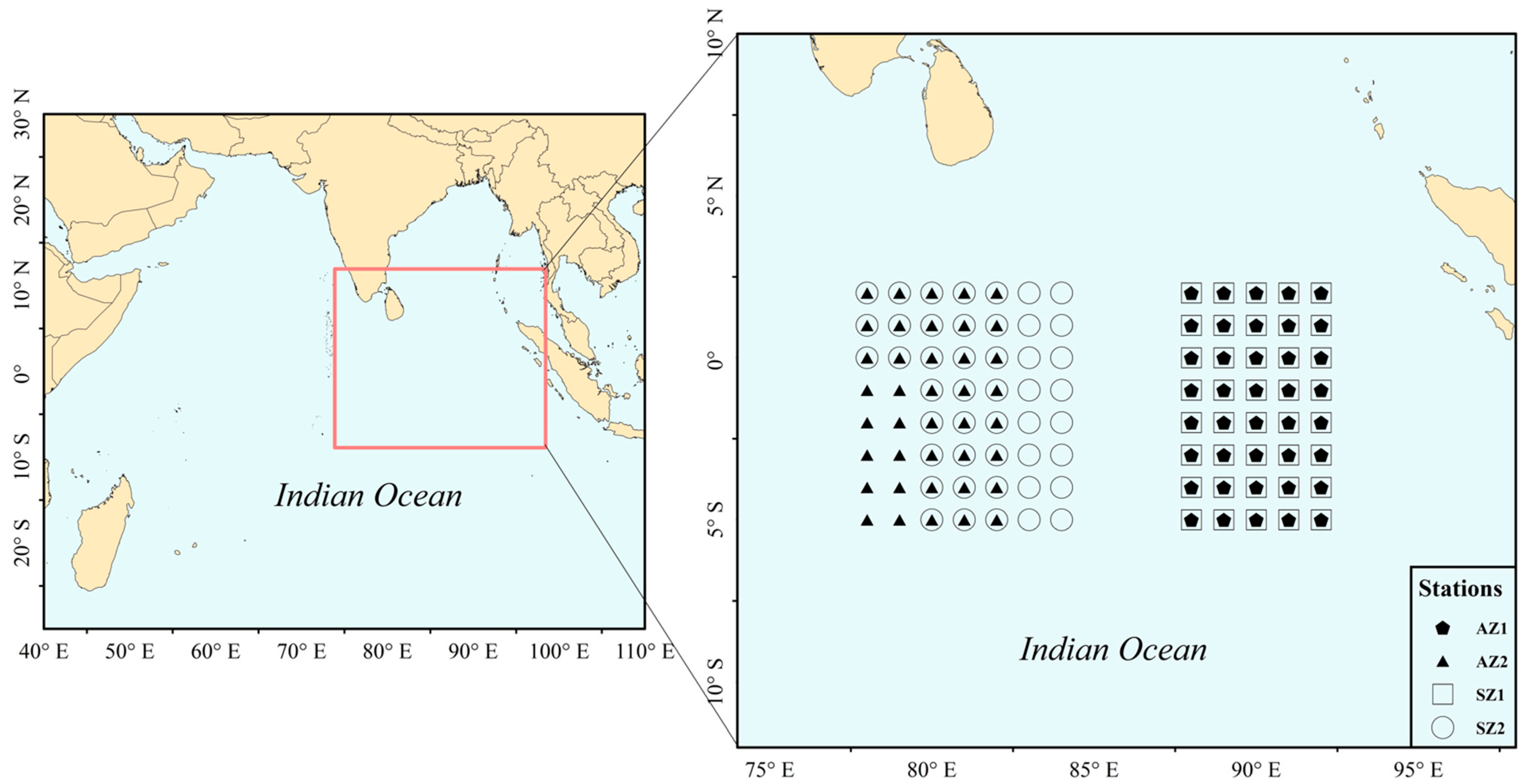
2.1. Fishery Data

The fishery data were obtained both spring and autumn surveys in the two zones of the east equatorial Indian Ocean. The survey area for zone 1 was from 5° N to 2° S, 88° E to 82° E, with the autumn survey from 17 September to 8 October 2019 and the spring survey from 16 May to 5 June 2021. The survey area for zone 2 was from 5° N to 2° S, 78° E to 84° E, with the autumn survey from 2 to 20 October 2020 and the spring survey from 4 to 26 May 2022. Except for zone 2’s spring survey, which had 46 stations, each of the other surveys included 40 stations (Figure 1).
Two light-lift-net fishing vessels named “Fuyuanyu 080” and “Fuyuanyu 082” were used for each survey. Both fishing vessels have identical specifications with 54.64 m length, 10.50 m width, 4.75 m draught, and 960 gross tonnages. Biological samples were collected during nighttime operations using a light-lift-net. The circumference of the mesh coat was 800 m, with a mesh size of the cod-end of 20 mm, and the mesh size of the net mouth was 40 mm.
The maximum effective fishing depth of the net was 50 m. Along the sides of the vessel, 110 attracting lamps (each with a power of 4 kW) were arranged in two rows. Catches were sorted by species, with random subsamples collected on deck. Subsequently, all sampled individuals were then transported to the laboratory for body weight measurements. The CPUE for each station was used as the abundance index for S. oualaniensis. Since the fishing effort of the light-lift-net was primarily determined by the duration of the attracting lamps’ operation, the CPUE for S. oualaniensis (in kg/h) was calculated by dividing the total catch of S. oualaniensis (in kg) by the duration of the light operation (in hours).

2.2. Environment Data

Sea temperature data were obtained using an SV48 conductivity–temperature–depth (CTD) profiler produced by Sea & Sun Technology GmbH (Trappenkamp, Germany). The CTD profiler was placed deeper than 100 m at each station. The data of SST and the sea temperature at 100 m depth (ST100) were extracted separately from the CTD profiler. The MLD was defined as the depth at which the temperature was 1 °C lower than the average temperature within 10 m of the surface layer [24].
Chla concentrations were determined through laboratory analysis of water samples collected in situ. Surface water samples were obtained at a depth of approximately 2 meters using a water sampler. Each sample consisted of 1 L of seawater, which was then filtered through the Whatman GF/F filter membrane (Φ 45 mm). The filter membranes were stored in darkness at −20 °C. After 20~24 h of extraction in 10 cm3 of 90% acetone under low temperature, the fluorescence was measured by the fluorometric method using a Turner Designs 10-Au Fluorometer (detection limit of 0.01 mg/m3). The Chla concentration was calculated based on the classical formula [25]. The relative error of the replicate samples was ±10% at the level of 0.5 mg/m3 for Chla concentration.
The daily SSH and geostrophic currents (u and v components), with a spatial resolution of 0.25°, were derived from Ocean Watch (https://coastwatch.pfeg.noaa.gov, accessed on 14 November 2024), and average values were calculated over the survey period. To represent the energy of sea surface current, the EKE was used, which is calculated from u and v with Equation (1) [22].
EKE = (u2 + v2)/2
where u and v represent the meridional and zonal components of the geostrophic current, respectively.

2.3. Data Analyses

The statistical analysis for differences in environmental factors of each survey was performed using the Kruskal–Wallis test for multi-group comparisons.
The Generalized Additive Model (GAM) was employed to analyze the response of S. oualaniensis to various environmental factors [26]. GAM exhibits a high degree of flexibility as it does not require any assumption about the functional form, merely demanding independence among the predictor variables. This makes it well-suited for analyzing spatiotemporal data and elucidating complex nonlinear relationships between the dependent variable and multiple independent variables.
To establish the optimal model, a stepwise regression approach was adopted. To avoid collinearity among environmental factors, Pearson correlation analysis was performed on the selected environmental indices. During the process of building the optimal model, models containing correlated factors (p < 0.001) were excluded to mitigate the issue of collinearity. The optimal model was chosen based on a comprehensive consideration of the Akaike Information Criterion (AIC) value and the number of model parameters. The equation for the GAM is as follows:
g (y) = β0 + f1 (x1) + f2 (x2) +⋯+ fn (xn) + factors + ϵ
where g is the link function, y is the dependent variable, β0 is the intercept, fi (xi) are smooth functions of the predictor variables xi (representing environmental factors), and ϵ is the error term. The smooth functions fi capture the nonlinear relationships between the response and the predictors without imposing a specific parametric form. In this study, CPUE was set as the dependent variable and environmental factors ware set as independent variables, while year, season, and zone were set as the factor variables. The CPUE was subjected to a log (CPUE + 1) transformation to conform to a normal distribution and utilize the 0-value. The GAM was completed using the MGCV package in R (version 3.6.1) [27].

3. Results

3.1. The Distribution of CPUE of S. oualaniensis

The average CPUE was significantly higher in autumn than in spring in zone 1, with 27.58 kg/h and 4.02 kg/h, respectively. There are 13 stations with a CPUE exceeding 30 kg/h in the zone 1 autumn survey, mainly located in the western and southern parts of zone 1, with the highest CPUE of 142.04 kg/h in 1° N, 88° E (Figure 2A and Figure 3A). However, there were no stations with a CPUE exceeding 30 kg/h in the zone 1 spring survey and only five stations exceeding 10 kg/h. Those stations mainly concentrated in the west-central part of the surveyed area, with the highest CPUE reaching 22.86 kg/h at 2° S, 91° E (Figure 2B and Figure 3B).
In contrast, the average CPUE in spring was significantly higher than that in autumn in zone 2, with 22.02 kg/h and 5.90 kg/h, respectively. There was only one station with a CPUE over 30 kg/h in AZ2, with 33.9 kg/h at 4°S, 80°E (Figure 2C and Figure 3C). In addition, there were five stations with a CPUE between 10 and 30 kg/h mainly distributed in the most southern and northern section of zone 2. There were 12 stations with a CPUE over 30 kg/h in the zone 2 spring survey (Figure 2D). Those stations mainly concentrated in the northern part of the surveyed area, with the highest CPUE reaching 91.25 kg/h at 1° S, 84° E (Figure 3D).

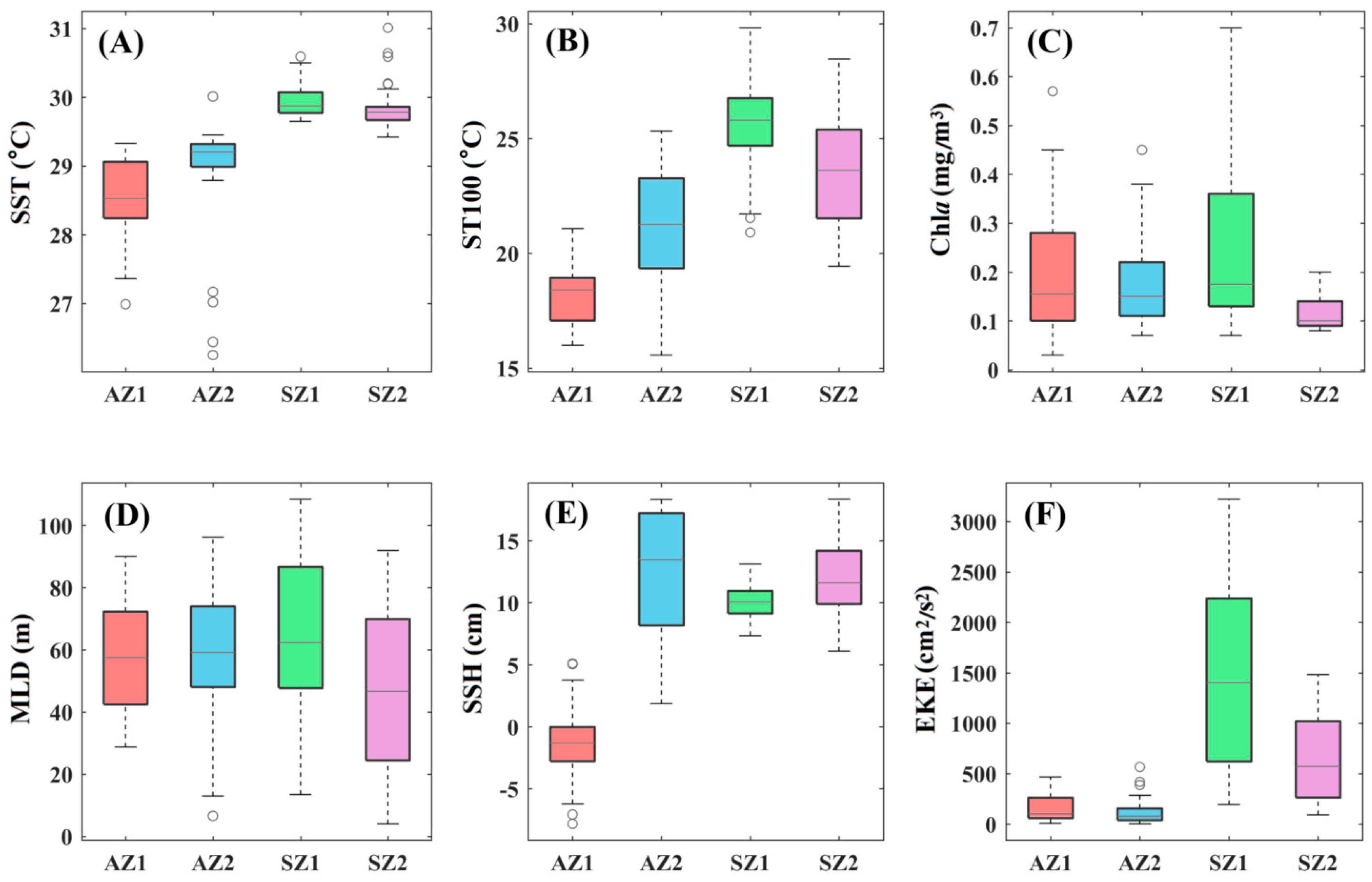
3.2. Environmental Factors at Survey Stations

Significant between-group differences (p < 0.05.) were demonstrated by the Kruskal–Wallis test for each environmental factor investigated. The Kruskal–Wallis chi-squared was highest for SST (122.79) and lowest for MLD (10.30). Across the four surveys, SST varied from 26.25 to 31.01 °C, with maximum and minimum medians occurring in the zone 1 spring survey and zone 1 autumn survey, respectively (Figure 4A). Both survey zones showed higher water temperatures in spring than in autumn. ST100 exhibited similar variations to SST, varying from 15.57 to 29.82 °C (Figure 4B). Chla varied from 0.03 to 0.70 mg/m3, with maximum and minimum medians occurring in the zone 1 spring survey and the zone 2 spring survey, respectively (Figure 4C). The MLD varied from 4.06 to 108.38 m, exhibiting similar trends to those of Chla (Figure 4D). SSH varied from −7.84 to 18.36 cm, with maximum and minimum medians occurring in the zone 2 autumn survey and zone 1 autumn survey, respectively (Figure 4E). The variation in SSH was shown by significantly higher values in zone 2 compared to zone 1. The EKE varied from 3.71 to 3220.91 m2/s2, with maximum and minimum medians occurring in the zone 1 spring survey and zone 2 autumn survey (Figure 4F). The variation in EKE was shown by significantly higher values in spring compared to autumn, with zone 1 being higher than zone 2.

3.3. GAM Analysis

The results of Pearson correlation analysis indicated that CPUE is significantly negatively correlated with ST100 and SSH at the p < 0.001 level (Figure 5). Significant correlations were also observed between multiple pairs of environmental factors, particularly between SST, ST100, and EKE.
The optimal CPUE prediction model was established using stepwise regression (Table 1). The single independent variable model with best fit and AIC values was constructed using SSH, with an adjusted R2 value of 0.327, explaining 30.1% of the deviance (Model 5 in Table 1). In the subsequent stepwise regression, to avoid covariance between the independent variables, factors correlated with SSH were excluded from the two independent variable models. The results indicated that the model with best fit and AIC values was constructed using the SSH and EKE, with an adjusted R2 value of 0.305, explaining 34.9% of the deviance (Model 9 in Table 1). Stepwise regression terminated as the remaining environmental factors were all correlated with EKE. Therefore, Model 9, with the two independent variables SSH and EKE, is the optimal model for predicting the CPUE of S. oualaniensis.
The response curves of each independent variable in the optimal model (model 9) to relative CPUEs were plotted (Figure 6). According to this model, the partial effect of SSH on CPUE is positive when SSH has values that are less than 0 cm (with the maximum CPUE occurring around an SSH of 0 cm). For SSH values between 0 cm and 0.1 cm, the partial effect becomes negative (with the lowest CPUE occurring around an SSH of 0.1 cm). The partial effect on CPUE is positive for SSH values between 0.1 cm and 0.14 cm, and then returns to being negative for SSH values greater than 0.14 cm (Figure 6A). In the same model, the partial effect of EKE on CPUE is positive when EKE values are less than 1200 m2/s2 (with the maximum CPUE occurring around an EKE of 1200 m2/s2). For EKE values higher than 1200 m2/s2, the effect becomes negative (Figure 6B).

4. Discussion

4.1. The Distribution of S. oualaniensis

S. oualaniensis is one of the most economically important cephalopods in the world, and its abundance and distribution have been of great interest [1]. Although S. oualaniensis is widely distributed in the Indo-Pacific equatorial waters, current research on S. oualaniensis has focused on the South China Sea and the Northwest Indian Ocean [8,9]. According to an assessment of S. oualaniensis in the Arabian Sea, the average abundance is 4.2 t/km2, with the maximum sustainable yield estimated as 0.63 million tons [4]. Tian et al. [18] showed that the average CPUE in the Northwest Indian Ocean is 5.24 t/d. Xie et al. [19] showed that the CPUE in the South China Sea is about 3 t/d. In order to understand the resource status of S. oualaniensis in the east equatorial Indian Ocean, this study conducted spring and autumn surveys in two zones, separately. The research showed that the average CPUE of S. oualaniensis in the surveyed zones was 14.55 kg/h, which is much lower than that in the South China Sea and the Northwest Indian Ocean [18,19]. Therefore, the current abundance of S. oualaniensis in the east equatorial Indian Ocean is not sufficient to be a good fishery ground. The low productivity of this region compared to the South China Sea and the Northwest Indian Ocean may be the main reason for the relatively low abundance of S. oualaniensis resources [28].
It is well known that S. oualaniensis also conducts daily vertical migration, migrating to the surface at night from a depth of 200 m [4]. In addition, further research has shown that the vertical migration of S. oualaniensis is most likely driven by the upward migration of preys such as chaetognaths [5,6]. In the sea survey of this study, the echo fish detection equipment can clearly observe the vertical migration behavior of S. oualaniensis. During the light-lift-net fishing during night, the average S. oualaniensis group would be gathered at depths of more than 50 m and eventually be caught. In this study, the CPUE of S. oualaniensis between the two zones showed an opposite seasonal variation: zone 1 had a significantly higher CPUE in the autumn than in the spring, while zone 2 showed the opposite trend. However, both zones shared a similar characteristic: in spring, the high-CPUE area was close to the continental shelf, whereas in autumn, it was farther from the continental shelf (Figure 3). Studies in the South China Sea have shown that S. oualaniensis undergoes seasonal migration, moving to shallow waters for spawning in spring and deep water for feeding in autumn [29]. Therefore, the seasonal shifts in the high-CPUE area observed in this study reflect the characteristics of its spawning–feeding migration pattern in the east equatorial Indian Ocean.

4.2. The Effect of Environmental Factors on the Distribution of S. oualaniensis

It has been revealed that marine environmental factors, including water temperature, salinity, food, and currents, have an important influence on the distribution of pelagic species [22,30,31]. In this study, six environmental factors were used to establish a GAM analysis with the CPUE of S. oualaniensis (Table 1). The models with a single independent variable (Models 1 to 6) showed that the environmental factor with the highest variance explanation was an SSH with 30.1%. The results indicated that SSH was the most important environmental factor affecting the CPUE of S. oualaniensis in this study.
SSH reflects dynamic environmental parameters such as sea level, sea current direction, and flow velocity [32]. An SSH value lower than the mean sea level indicates a divergence or upwelling of ocean currents, which leads to the continuous replenishment of nutrient-rich waters from the bottom layers to the surface, thereby promoting the growth, development, and reproduction of S. oualaniensis [3,33]. The formation of the S. oualaniensis habitat in the Northwest Indian Ocean has been shown to be influenced by upwelling, which carries nutrient-rich water from the deeper layers to the upper layers, increasing productivity and Chla concentrations in the region [34,35]. Furthermore, numerous observations and practices have revealed that high-density fish populations are not distributed in the central areas of upwelling with the highest plankton concentrations but rather in the periphery of the upwelling or in the center of the downwelling [33,35,36]. Similar patterns have been observed in studies of the S. oualaniensis. The exploratory fishery for S. oualaniensis in the Indian Ocean from 2004 to 2005 showed that most of the high-catch centers were located in the area with an SSH less than 0 m, and the centers were distributed on the cold-water eddy side of the confluence of the cold and warm eddies [37]. This is consistent with the results of the present study that a lower SSH favors the aggregation of S. oualaniensis.
The results of the GAM in this study show that in addition to SSH, EKE is included in the optimal model. The EKE is a reflection of the velocity of the sea current in the horizontal direction, which plays a pivotal role in transporting highly productive offshore water masses to deeper and more distant seas, thereby enhancing productivity in proximity to these currents [38,39]. Several studies have demonstrated a robust influence of EKE on the formation of fisheries [20,40]. Furthermore, currents facilitate the dissemination of eggs and larvae of S. oualaniensis, while also providing suitable food sources and habitats for the adults [22]. Certain specific current systems, including oceanic circulation and coastal currents, exert additional influences on the migration routes and distribution patterns of S. oualaniensis [37].
Water temperature is generally regarded as a crucial factor influencing the distribution of S. oualaniensis [14]. The pivotal role of suitable SST ranges in determining habitat preferences of S. oualaniensis varies across different growth stages [15]. Furthermore, seasonal changes in SST can lead to migrations in the distribution of S. oualaniensis, spreading to cooler waters during the warm season and vice versa during the cold season [6,34]. In this study, besides SST, two other temperature-related factors, ST100 and MLD, were also considered. Several studies have indicated that water temperature at deeper layers may have a more significant impact on fish distribution than surface temperatures [41,42]. Yan Lei et al. [43] conducted a Gray Relational Analysis on S. oualaniensis in the South China Sea, revealing that the vertical temperature gradient between 5 and 50 m is the most influential factor affecting S. oualaniensis yield. Specifically, S. oualaniensis yield decreased with an increase in the vertical temperature gradient in spring, whereas the average squid yield increased with an increase in the vertical temperature gradient in autumn.
In this study, the results of the GAMs revealed that SST and ST100 factors exhibited a relatively high variance explanation, accounting for 13.9% and 13.2%, respectively, of the CPUE of S. oualaniensis. Furthermore, the Pearson correlation analysis indicated a significant negative correlation between ST100 and the CPUE of S. oualaniensis, confirming that a lower ST100, or equivalently a higher temperature gradient, corresponded to a higher CPUE. However, both SST and ST100 were found to be correlated with SSH, and the AIC values for the single-independent-variable models were higher than that for the SSH model. This could be attributed to the fact that the surveyed zones are located in the equatorial zone, where water temperature variations are relatively minimal, leading to a weaker explanatory power of temperature (Figure 4). Given that the independent variables in the model should be uncorrelated, these factors were excluded from the optimal GAM.
In addition to marine environmental factors, biological factors are intimately tied to the distribution patterns of S. oualaniensis [10,44]. As a crucial component within the marine food chain, the distribution of S. oualaniensis is significantly influenced by the availability and distribution of its prey and natural predators. For instance, abundant zooplankton and small fish resources often serve as attractants, drawing S. oualaniensis into aggregations, whereas the presence of natural predators may prompt them to steer clear of specific regions [45]. Therefore, it is imperative to incorporate biological factors into future investigations to gain a more comprehensive understanding of the distributional mechanisms underlying S. oualaniensis.

5. Conclusions

This study utilized light-lift-net fishing vessels to conduct spring and autumn surveys in two separate zones in the eastern equatorial Indian Ocean. The survey results showed that the average CPUE of S. oualaniensis for the four surveys, in descending order, was the zone 1 autumn survey (27.58 kg/h), zone 2 spring survey (22.02 kg/h), zone 2 autumn survey (5.90 kg/h), and zone 1 spring survey (4.02 kg/h). The average CPUE of S. oualaniensis across the four surveys was 14.55 kg/h, which was considerably lower than in the South China Sea and Northwest Indian Ocean. In terms of the seasonal distribution of CPUE, there is a trend of spawning migration from closer to the continental shelf in spring to deeper and offshore waters in autumn. Pearson correlation analysis showed that the CPUE of S. oualaniensis reflected a significant negative correlation with both ST100 and EKE (p < 0.001). Furthermore, the GAM revealed that SSH was the most significant factor affecting the CPUE of S. oualaniensis with a 30.1% variance explanation, and the optimal prediction model includes two factors, SSH and EKE, with a variance explanation of 34.9%. These findings revealed the distribution and seasonal variations of S. oualaniensis in the eastern equatorial Indian Ocean, as well as its response to the marine environment.

Author Contributions

Conceptualization, S.L., L.Z., P.S., R.W. and Y.L.; data curation, S.L. and L.Z.; formal analysis, S.L. and R.W.; funding acquisition, S.L., L.L. and Y.L.; investigation, S.L., J.K., P.S., X.M. and Y.L.; methodology, S.L., L.Z. and P.L.; project administration, L.L. and Y.L.; resources, L.L.; software, S.L. and R.W.; supervision, L.L. and Y.L.; validation, S.L., L.Z. and R.W.; visualization, S.L.; writing—original draft preparation, S.L., L.Z., J.K. and R.W.; writing—review and editing, Y.L. All authors have read and agreed to the published version of the manuscript.

Funding

This study was supported by the National Key Research and Development Program of China (2023YFF0611803), the Scientific Research Foundation of the Third Institute of Oceanography, MNR (2023019), the National Programme on Global Change and Air-Sea Interaction (GASI-01-EIND-YD01/02aut/spr), and The central public-interest scientific Institution basal research Fund from the Chinese Academy of Fishery Sciences (2023TD12).

Institutional Review Board Statement

The animal study of our manuscript was reviewed and approved by the Ethics Committee of the Third Marine Institute, Ministry of Natural Resources, (Approval Code: TIO-IACUC-01-2024-11-08; Approval Date: 8 November 2024.).

Data Availability Statement

The datasets generated and analyzed during the current study are available from the corresponding author upon reasonable request.

Conflicts of Interest

All authors acknowledge that there are no conflicts of interest with their involvement and publication of this work.

References

  1. Dunning, M.C. A Review of Systematics, Distribution and Biology of the Arrow Squid Genera Ommastrephes d’Orbigny, 1835, Sthenoteuthis Verrill, 1880 and Ornithoteuthis Okada, 1927 (Cephalopoda: Ommastrephidae); Voss, N.A., Vecchione, M., Toll, R.B., Sweeney, M.J., Eds.; Systematics and Biogeography of Cephalopods; Smithsonian University Press: Washington, DC, USA, 1998; pp. 425–433. [Google Scholar]
  2. Chen, X.; Liu, B.; Tian, S.; Qian, W.; Zhao, X. Fishery Biology of Purpleback Squid, Sthenoteuthis oualaniensis, in the Northwest Indian Ocean. Fish. Res. 2007, 83, 98–104. [Google Scholar]
  3. Trotsenko, B.G.; Pinchukov, M.A. Mesoscale distribution features of the purpleblack squid Sthenoteuthis oualaniensis with reference to the structure of the upper quasi-homogeneous layer in theWest India Ocean. Oceanology 1994, 34, 380–385. [Google Scholar]
  4. Kurichithara, K.K.; Najmudeen, T.M.; Ragesh, N.; Jeena, N.S.; Rahuman, S.; Sunil, K.S.; Sasikumar, G.; Mohamed, K.S. Characterisation of an individual of the giant form of the purpleback flying squid Sthenoteuthis oualaniensis (Cephalopoda: Ommastriphidae) in the Arabian Sea and its biological descriptors. Molluscan Res. 2021, 41, 275–284. [Google Scholar]
  5. Young, R.E.; Hirota, J. Review of the ecology of Sthenoteuthis oualaniensis near the Hawaiian Archipelago. In Contributed Papers to International Symposium on Large Pelagic Squids; Japan Marine Fishery Resources Research Center: Tokyo, Japan, 1998; pp. 113–143. [Google Scholar]
  6. Fan, J.; Chen, Z.; Feng, X.; Yu, W. Climate-related changes in seasonal habitat pattern of Sthenoteuthis oualaniensis in the South China Sea. Ecosyst. Health Sustain. 2021, 7, 1926338. [Google Scholar] [CrossRef]
  7. Nigmatullin, C.M. Resources and perspectives of the fisheries of nektonic epipelagic squids in the World Ocean. In Abstracts of the All-Union Conference on Reserve Food Biological Resources of the Open Ocean and Seas of the USSR, Kaliningrad, 1990; MIK: Moscow, Russia, 1990; pp. 11–13. [Google Scholar]
  8. Mohamed, K.S.; Sasikumar, G.; Koya, K.P.S.; Venkatesan, V.; Kripa, V.; Durgekar, N.R.; Joseph, M.; Alloycious, P.S.; Mani, R.; Vijay, D. Know… The Master of the Arabian Sea—Purple-Back Flying Squid Sthenoteuthis oualaniensis; ICAR—Central Marine Fisheries Research Institute: Kochi, India, 2011. [Google Scholar]
  9. Zhang, J.; Chen, Z.; Chen, G.; Qiu, Y.; Liu, S.; Yao, S. Hydroacoustic Detection and Estimation Techniques of Squid Sthenoteuthis oualaniensis in the South China Sea. South China Fish. Sci. 2014, 10, 1–11. [Google Scholar]
  10. Gong, Y.; Zhan, F.; Yang, Y.; Zhang, P.; Kong, X.; Jiang, Y.; Chen, Z. Feeding habits of Symplectoteuthis oualaniensis in the South China Sea. South China Fish. Sci. 2016, 12, 80–87. [Google Scholar]
  11. André, J.; Haddon, M.; Pecl, G.T. Modelling climate-change-induced nonlinear thresholds in cephalopod population dynamics. Glob. Change Biol. 2010, 16, 2866–2875. [Google Scholar] [CrossRef]
  12. Pang, Y.; Tian, Y.; Fu, C.; Wang, B.; Li, J.; Ren, Y.; Wan, R. Variability of coastal cephalopods in overexploited China Seas under climate change with implications on fisheries management. Fish. Res. 2018, 208, 22–33. [Google Scholar] [CrossRef]
  13. Ma, S.; Cheng, J.; Li, J.; Liu, Y.; Wan, R.; Tian, Y. Interannual to decadal variability in the catches of small pelagic fishes from China seas and its responses to climatic regime shifts. Deep-Sea Res. II Top. Stud. Oceanogr. 2019, 159, 112–129. [Google Scholar] [CrossRef]
  14. Han, H.; Jiang, B.; Shi, Y.; Jiang, P.; Zhang, H.; Shang, C.; Sun, Y.; Li, Y.; Xiang, D. Response of the Northwest Indian Ocean purpleback flying squid (Sthenoteuthis oualaniensis) fishing grounds to marine environmental changes and its prediction model construction based on multi-models and multi-spatial and temporal scales. Ecol. Indic. 2023, 154, 110809. [Google Scholar] [CrossRef]
  15. Su, L.; Chen, Z.; Zhang, P. Reproductive biology of purpleback flying squid (Symplectoteuthis oualaniensis) in the south-central South China Sea in spring and autumn. South China Fish. Sci. 2016, 12, 96–102. [Google Scholar]
  16. Zhou, W.; Xu, H.; Li, A.; Cui, X.; Chen, G. Comparison of habitat suitability index models for purpleback flying squid (Sthenoteuthis oualaniensis) in the open South China Sea. Appl. Ecol. Env. Res. 2019, 17, 4903–4913. [Google Scholar] [CrossRef]
  17. Guo, Y.; Wu, W.; Ling, W.; Zhao, C.; Feng, B.; Yan, Y. Relationship between CPUE of Sthenoteuthis oualaniensis and environmental factors in the southeastern Coast of Hainan in Spring. J. Guangdong Ocean Univ. 2020, 40, 63–70. [Google Scholar]
  18. Tian, S.; Chen, X.; Yang, X. Study on the Fishing Ground Distribution of Symlectoteuthis oualaniensis and Its Relationship with the Environmental Factors in the High Sea of the Northern Arabian Sea. Trans. Oceanogr. Limnol. 2006, 1, 51–57. [Google Scholar]
  19. Xie, E.; Zhou, Y.; Feng, F.; Wu, Q. Catch per unit effort (CPUE) standardization of purpleback flying squid Sthenoteuthis oualaniensis for Chinese large-scale lighting net fishery in the open sea of South China Sea. J. Dalian Ocean Univ. 2020, 35, 439–446. [Google Scholar]
  20. Mugo, R.; Saitoh, S.I.; Nihira, A.; Kuroyama, T. Habitat characteristics of skipjack tuna (Katsuwonus pelamis) in the western North Pacific: A remote sensing perspective. Fish. Oceanogr. 2010, 19, 382–396. [Google Scholar] [CrossRef]
  21. Yu, W.; Chen, X.; Chen, Y.; Yi, Q.; Zhang, Y. Effects of environmental variations on the abundance of western winter-spring cohort of neon flying squid (Ommastrephes bartramii) in the Northwest Pacific Ocean. Acta Oceanol. Sin. 2015, 34, 43–51. [Google Scholar] [CrossRef]
  22. Liu, S.; Liu, Y.; Li, J.; Cao, C.; Tian, H.; Li, W.; Tian, Y.; Watanabe, Y.; Lin, L.; Li, Y. Effects of oceanographic environment on the distribution and migration of Pacific saury (Cololabis saira) during main fishing season. Sci. Rep. 2022, 12, 13585. [Google Scholar] [CrossRef]
  23. Yu, W.; Wen, J.; Chen, X.; Gong, Y.; Liu, B. Trans-Pacific multidecadal changes of habitat patterns of two squid species. Fish. Res. 2021, 233, 105762. [Google Scholar] [CrossRef]
  24. Shi, P.; Du, Y.; Wang, D.; Gan, Z. Annual cycle of mixed layer in South China Sea. J. Trop. Oceanogr. 2001, 20, 10–17. [Google Scholar]
  25. Yentsch, C.S.; Menzel, D.W. A method for the determination of phytoplankton chlorophyll and phaeophytin by fluorescence. Deep Sea Res. Oceanogr. Abstr. 1963, 10, 221–231. [Google Scholar] [CrossRef]
  26. Hastie, T.; Tibshirani, R. Generalized additive models: Some applications. J. Am. Stat. Assoc. 1987, 82, 371–386. [Google Scholar] [CrossRef]
  27. R Core Team. R: A Language and Environment for Statistical Computing; Foundation for Statistical Computing: Vienna, Austria, 2013. [Google Scholar]
  28. Stock, C.A.; John, J.G.; Rykaczewski, R.R.; Asch, R.G.; Cheung, W.W.; Dunne, J.P.; Friedland, K.D.; Lam, V.W.Y.; Sarmiento, J.L.; Watson, R.A. Reconciling fisheries catch and ocean productivity. Proc. Natl. Acad. Sci. USA 2017, 114, E1441–E1449. [Google Scholar] [CrossRef] [PubMed]
  29. Yu, J.; Hu, Q.; Tang, D.; Zhao, H.; Chen, P. Response of Sthenoteuthis oualaniensis to marine environmental changes in the north-central South China Sea based on satellite and in situ observations. PLoS ONE 2019, 14, e0211474. [Google Scholar] [CrossRef]
  30. Xing, Q.; Yu, H.; Liu, Y.; Li, J.; Tian, Y.; Bakun, A.; Cao, C.; Tian, H.; Li, W. Application of a fish habitat model considering mesoscale oceanographic features in evaluating climatic impact on distribution and abundance of Pacific saury (Cololabis saira). Prog. Oceanogr. 2022, 201, 102743. [Google Scholar] [CrossRef]
  31. Liu, S.; Li, Y.; Wang, R.; Miao, X.; Zhang, R.; Chen, S.; Song, P.; Lin, L. Effects of Vertical Water Column Temperature on Distribution of Juvenile Tuna Species in the South China Sea. Fishes 2023, 8, 135. [Google Scholar] [CrossRef]
  32. Killworth, P.D.; Dieterich, C.; Le Provost, C.; Oschlies, A.; Willebrand, J. Assimilation of altimetric data and mean sea surface height into an eddy-permitting model of the North Atlantic. Prog. Oceanogr. 2001, 48, 313–335. [Google Scholar] [CrossRef]
  33. Xing, Q.; Yu, H.; Wang, H.; Ito, S.-I.; Chai, F. Mesoscale eddies modulate the dynamics of human fishing activities in the global midlatitude ocean. Fish and Fish. 2023, 24, 527–543. [Google Scholar] [CrossRef]
  34. Yang, X.; Chen, X.; Zhou, Y.; Tian, S. A marine remote sensing-based preliminary analysis on the fishing ground of purple flying squid Sthenoteuthis oualaniensis in the northwest Indian Ocean. J. Fish. China 2006, 30, 669–675. [Google Scholar]
  35. Fu, Y.; Wu, X.; Jin, P.; Yu, W. Impacts of mesoscale eddies on the spatial and temporal distribution of Sthenoteuthis oualaniensis in the Northwest Indian Ocean. J. Fish. Sci. China 2024, 31, 454–464. [Google Scholar]
  36. Bakun, A. Ocean eddies, predator pits and bluefin tuna: Implications of an inferred ‘low risk–limited payoff’ reproductive scheme of a (former) archetypical top predator. Fish Fish. 2013, 14, 424–438. [Google Scholar] [CrossRef]
  37. Shao, F.; Chen, X. Relationship between fishing ground of Symlectoteuthis oualaniensis and sea surface height in the northwest Indian ocean. Mar. Sci. 2008, 32, 88–92. [Google Scholar]
  38. Appen, W.J.V.; Baumann, T.M.; Janout, M.; Koldunov, N.; Lenn, Y.D.; Pickart, R.S.; Scott, R.B.; Wang, Q. Eddies and the Distribution of Eddy Kinetic Energy in the Arctic Ocean. Oceanogr. 2022, 35, 42–51. [Google Scholar] [CrossRef]
  39. Wang, T.; Du, Y.; Adeagbo, Z.O.S. Influence of rossby wave in southern Indian Ocean on the low frequency variability of eddy kinetic energy within agulhas current system. Deep-Sea Res. I Oceanogr. Res. Pap. 2024, 203, 104218. [Google Scholar] [CrossRef]
  40. Syah, A.F.; Saitoh, S.-I.; Alabia, I.D.; Hirawake, T. Detection of potential fishing zone for Pacific saury (Cololabis saira) using generalized additive model and remotely sensed data. IOP Conf. Ser. Earth Environ. Sci. 2017, 54, 012074. [Google Scholar] [CrossRef]
  41. Lan, K.W.; Lee, M.A.; Nishida, T.; Lu, H.J.; Weng, J.-S.; Chang, Y. Environmental effects on yellowfin tuna catch by the Taiwan longline fishery in the Arabian Sea. Int. J. Remote Sens. 2012, 33, 7491–7506. [Google Scholar] [CrossRef]
  42. Wang, L.; Li, Y.; Zhang, R.; Tian, Y.; Zhang, J.; Lin, L. Relationship between the resource distribution of Scomber japonicus and seawater temperature vertical structure of Northwestern Pacific Ocean. Period. Ocean Univ. China 2019, 49, 29–38. [Google Scholar]
  43. Yan, L.; Zhang, P.; Yang, B.; Chen, S.; Li, Y.; Li, Y.; Song, P.; Lin, L. Relationship between the catch of Symplectoteuthis oualaniensis and surface temperature and the vertical temperature structure in the South China Sea. J. Fish. Sci. China 2016, 23, 469–477. [Google Scholar]
  44. Wei, J.; Cui, G.; Xuan, W.; Tao, Y.; Su, S.; Zhu, W. Effects of SST and Chl-a on the spatiotemporal distribution of Sthenoteuthis oualaniensis fishing ground in the Northwest Indian Ocean. J. Fish. Sci. China 2022, 29, 388–397. [Google Scholar]
  45. Qian, W.G.; Chen, X.J.; Liu, B.L.; Tian, S.; Ye, X. The relationship between fishing ground distribution of Symlectoteuthis oualaniensis and zooplankton in the northwestern Indian Ocean in autumn. Mar. Fish. 2006, 28, 265–271. [Google Scholar]
Figure 1. Distribution of stations from zone 1 autumn survey (AZ1, 2019), zone 2 autumn survey (AZ2, 2020), zone 1 spring survey (SZ1, 2021), and zone 2 spring survey (SZ2, 2022).
Fishes 10 00184 g001
Figure 2. Frequency distribution of S. oualaniensis CPUE from (A) zone 1 autumn survey (2019), (B) zone 2 autumn survey (2020), (C) zone 1 spring survey (2021), and (D) zone 2 spring survey (2022).
Fishes 10 00184 g002
Figure 3. Distribution of S. oualaniensis CPUE from (A) zone 1 autumn survey (2019), (B) zone 1 spring survey (2021), (C) zone 2 autumn survey (2020), and (D) zone 2 spring survey (2022).
Fishes 10 00184 g003
Figure 4. Box plots of environmental factors in the stations of zone 1 in the autumn survey (AZ1, 2019), zone 2 in the autumn survey (AZ2, 2020), zone 1 in the spring survey (SZ1, 2021), and zone 2 in the spring survey (SZ2, 2022). (A) Sea surface temperature (SST), (B) sea temperature at a depth of 100 m (ST100), (C) sea surface chlorophyll-a concentration (Chla), (D) mixed layer depth (MLD), (E) sea surface height (SSH), and (F) eddy kinetic energy (EKE). Boxes represent the interquartile range (IQR), which covers the middle 50% of the data (from the 25th to the 75th percentile). The line inside the box marks the median (50th percentile). The whiskers extend to the minimum and maximum values within 1.5 times the IQR, and any dots beyond the whiskers indicate potential outliers.
Fishes 10 00184 g004
Figure 5. Correlation analysis among S. oualaniensis CPUE and environmental factors. The figure presents bivariate scatterplots with fitted lines in the lower panels, single-variable histograms along the diagonal, and Pearson correlation coefficients in the upper panels. Significant correlations (p < 0.001) are highlighted in bold red font.
Fishes 10 00184 g005
Figure 6. Impact of SSH (A) and EKE (B) on CPUE of S. oualaniensis in optimal GAM.
Fishes 10 00184 g006
Table 1. GAM stepwise statistical regression parameters of S. oualaniensis.
ModelCovariantDegree of FreedomAIC ValueVariance Explanation %R-Sq. (adj)
1SST4.15247.0713.900.11
2ST1001.00242.0013.200.12
3Chla1.00255.325.810.04
4MLD2.32259.225.080.03
5SSH5.59214.2330.100.37
6EKE3.15247.0012.800.10
7SSH + Chla6.91214.7331.700.28
8SSH + MLD7.92215.0432.400.28
9SSH + EKE8.35209.7234.900.31
Disclaimer/Publisher’s Note: The statements, opinions and data contained in all publications are solely those of the individual author(s) and contributor(s) and not of MDPI and/or the editor(s). MDPI and/or the editor(s) disclaim responsibility for any injury to people or property resulting from any ideas, methods, instructions or products referred to in the content.

