Abstract
To describe the growth pattern of the bonnethead shark (Sphyrna tiburo) in the Gulf of Mexico, a von Bertalanffy (VB) model has been automatically fit, which indicated a single−phase continuous growth without oscillations, though this would generate biases if this hypothesis is not confirmed. The objective of this research was to describe the growth pattern of S. tiburo under a multimodel approach based on information theory and contrasting single−phase models (VB, Gompertz, logistic models, and variants) and biphasic models (Soriano model and variants). The VB model was not supported. The Soriano model, with the variant in growth rate (k) and including length at birth (L0), was selected with 100% supporting evidence. The hypothesis of the two−phase growth of S. tiburo with an increase in k, more than L∞, fitted to L0, is confirmed, and a correspondence was identified between growth−phase change sizes and the sizes reported in the literature for change in the juvenile–adult stages in females and for onset of reproductive maturity in males and both sexes.
1. Introduction
Along the coast of the Gulf of Mexico (GM) coexist several highly important fisheries, including of the Atlantic sharpnose shark (Rhizoprionodon terraenovae) [1]. In the particular case from the coast of Tamaulipas, Mexico, this fishing resource ranks 10th in value and volume among the main fisheries from the state [2]. Specifically, the bonnethead shark Sphyrna tiburo [3] represents 50% of the total volume contributed by the group of small coastal sharks in the southeastern United States and 15% of the volume of the annual catch in the GM [4]. Recently, it was found that the bonnethead shark, along with the Atlantic sharpnose shark, were the two most captured shark species in the southeastern GM [5].
In the coast of Tamaulipas are found the group of dogfish sharks made up of the following species: Atlantic sharpnose shark, bonnethead shark, blacknose shark (Carcharhinus acronotus) [6] and porous shark (C. porosus) [7], characterized by being small in size (<150 cm in total length) and recognized as a species of “high biological productivity” for having a rapid growth rate, high reproductive potential and reaching the age of first maturity during their first four years of life [8,9].
In this same coastal region, as in the rest of Mexico, there is a commercial shark fishery, managed through commercial fishing permits, which is why it represents a directed fishery, whose target species are sharks. This shark fishery in Mexico is represented by three fishery units: the coastal artisanal fishery that is carried out along the two sea coasts with vessels smaller than 10.5 m in length, which contributes to approximately 40% of national production; the medium height one, which is carried out with boats between 10 and 27 m in length in coastal waters on both coasts; and deep−sea fishing in which vessels of more than 27 m in length operate to capture sharks both in coastal waters and in oceanic waters within the Exclusive Economic Zone of the Pacific Ocean [10].
The bonnethead shark, the Atlantic sharpnose shark, the blacknose shark, and the finetooth shark Carcharhinus isodon [11] make up the group of small coastal sharks [12] on the east coast of the United States of America. S. tiburo is a very abundant small shark that is found in shallow waters such as the estuaries and bays of the coasts of the Atlantic and Pacific oceans of the Americas, including the GM [13], and whose regional migrations show spatial and temporal variations [14].
In the modelling of fish growth, it is generally chosen a priori to fit the von Bertalanffy model to the data of observed age frequencies [15,16], so it is assumed that the fish species follow an isometric growth pattern without oscillations and with continuity at all ages; sharks are no exception [17]. This a priori choice carries with it the risk of overestimating or underestimating parameters. Therefore, it is always advisable to test more than one growth model to find the one that best describes the observed data [18,19]. There is a rising trend in growth model selection, and specifically in multimodel inference, of estimating average parameters based on the specific statistical weight of each model [16].
In most vertebrate and plant growth investigations, the growth pattern is described as a single curve [20], but this approach has been criticized [21]. The most common single phase models (Von Bertalanffy, Logistic, and Gompertz) are generally easy to fit and generally apply to length-at-age data. In the case of fish, a criticism of these models is that growth throughout life comprises two or more stages that result from reproductive investment [21,22,23] or changes in habitat, food, or other stressors [21,24,25]. Describing these stages with a single curve can obscure important ecological and evolutionary information [21]. This is how the two state or biphasic models arise, where the growth acceleration generally changes around a transition age [26]. Such biphasic models have already been successfully applied to elasmobranch species, where such transitions are detectable only from length-at-age data [21]. It is important to estimate the growth parameters because they are inputs for the estimation methods of the instantaneous rates of total, natural and fishing mortality, directly, and they also represent inputs for the predictive models of yield per recruit of Beverton and Holt [27] and Thompson and Bell [28], directly and indirectly, respectively.
Research on the growth of S. tiburo is scarce. It has been studied on both sides (east and west) of the state of Florida, USA [29,30,31,32]. With the exception of Frazier et al. [32], all studies have chosen a priori to use the VB model to fit the data and model the growth pattern of the species, but biases will arise if this model is not confirmed to be right. Frazier et al. [32], in their research on the species in the Atlantic Ocean (east side of Florida), have been the only ones that have used the multimodel approach along with information theory to choose the model with the best fit for this species. They did not apply multimodel inference, and even though it was not the best model, they selected the VB model based on one biological criterion. It is presumed that in the west of the GM, S. tiburo has two growth phases.
The objective of the present study was to describe the growth pattern of the bonnethead shark S. tiburo of western GM under the multimodel approach, fitting single phase and biphasic models and making use of information theory to choose the best fitting model or applying the multimodel inference, as needed, to provide more robust estimates of its growth parameters.
2. Materials and Methods
2.1. Study Area
Samples of artisanal fishing were carried out in the Carbajal Fishing Zone, in the Municipality of San Fernando and in the towns of La Pesca and Miguel de la Madrid Hurtado (El Canal) in the Municipality of Soto La Marina, Tamaulipas, Mexico (Figure 1), from September 2016 to April 2019. The fishing gear used was mainly longlines and cazonera (shark) nets. The longlines were monofilaments with lengths between 600 and 1500 m on average and included snoods of 1.5 to 2.5 m in length, between 150 and 500 on average per longline, and between 350 and 750 “eagle claw” size 5–6 hooks per longline. The cazoneras were made of nylon and polyethylene, with lengths between 450 and 1000 m, a drop of 6 m, and a mesh opening of 12.5 cm. The sex of each captured organism was determined by the presence or absence of the (male) myxopterygium (copulatory organ). The total length (TL) in centimeters and the gutted weight in kilograms were taken with an ichthyometer (±1 mm) 1 m in length, graduated at every millimeter, and a Torrey OLEQ5−N digital scale with a capacity of 5 kg (± 0.1 g), respectively.
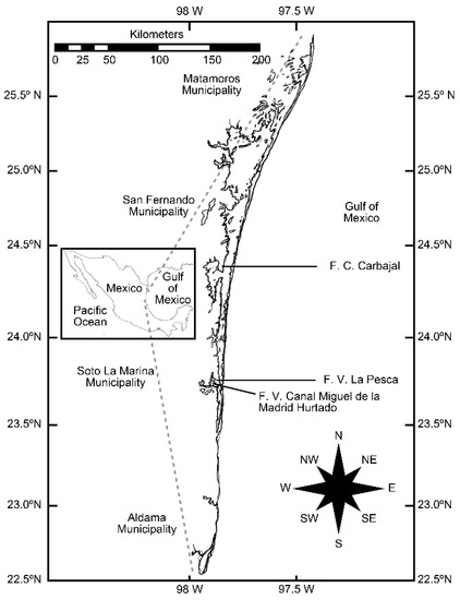
Figure 1.
Sampling sites of the bonnethead shark Sphyrna tiburo in the western Gulf of Mexico.
2.2. Multinomial Analysis
The modes present in the size distribution of the annual samples of females, males, and the total catches were determined through multinomial distribution with the following density probability function [33]:
where is the number of times that an i−type event occurs in n samples, n is the sample size, and is the probability of the i−type event. Haddon (2001) recommends that to estimate the parameters of the model, the equation must be converted into a likelihood expression as follows:
The main assumption underlying the estimation of the parameters is that the size distribution for each average or modal length assumes a normal distribution, each mode corresponding to a different cohort in the population. Under this condition, the estimates of the expected relative proportions of each length category were described through the following density function:
where and are the mean and standard deviation of the total length of each cohort, respectively. The starting values of the parameters in the previous equation were assigned according to a visual inspection of the frequency distributions of the data [34]. Then, to estimate the expected frequencies and the parameters of the models, the estimated and observed values were contrasted through the negative of the logarithm function of the maximum likelihood of the multinomial distribution [33,35]:
where the parameters and correspond to the mean and standard deviation of the total length corresponding to the n means that are present in the length distribution. The model parameters were estimated when the likelihood function (the latter expression) was minimized with Newton’s direct search algorithm [36].
2.3. Age Determination
For age determination, the separation index (SI) of a mean greater than 2 was used, according to Sparre and Venema [37] and the following equation:
where and correspond to the mean and standard deviation of the total length. In the first year of life, the bonnethead shark S. tiburo reaches 58.69 cm on average in females (range 50.73 to 62.38 cm), while in males the average size reached is 56.99 cm (range 41.17 to 62.32 cm), in Tampa Bay, Florida [38]. The smallest TLs observed in the modes obtained in this study (female = 56.02 cm and male = 59.43 cm) lie within these confidence intervals, so it was assumed that the TLs we found corresponded to the first year of life of S. tiburo.
2.4. Candidate Models
To identify the model that best described the growth of S. tiburo, 13 models were fit to the three data series (females, males, and both) of average TL of the modes and their correlative ages to estimate the growth parameters of each model and of the average models (Table 1). Seven models were applied in their basic forms, as were eight variants of them. The models fit in their basic form were von Bertalanffy [39], Soriano et al. [40] (S), Gompertz [41] (G), Johnson [42] (J), and logistic [41] (L). Variations of all the models but J were tested. The variation was done by substituting the parameter t0 by the parameter L0, according to the algorithm of each model with its respective source. In sum, the 13 models were VB1, VB2, S1, S2, S3, S4, S5, S6, G1 [43], G2 [44], J, L1, and L2 (Table 1). S and its variants were biphasic models, and the other models and their variants were single−phase models. These models were selected because they have been used traditionally to describe growth in fishes such as sharks.

Table 1.
A comparison of models describing the growth pattern of the bonnethead shark (Sphyrna tiburo) in the western Gulf of Mexico.
2.5. Model Fitting
The models were fit using an iterative process with the Excel solver function that used Newton’s direct search algorithm [36], assuming the types of error in the residuals were additive and multiplicative and maximizing the objective likelihood function [33]:
where = model parameters and = standard deviation of the error, calculated using the following equations:
, for the additive error, and for the multiplicative error, where TL = total length observed and = total length estimated. When the analysis was performed using the multiplicative error for the modelling, σ and were recalculated at an additive error scale to obtain consistent scales and comparable information criteria (indicated below).
2.6. Selection of Models
For the selection of models, the Akaike information criterion (AIC) was used [45] in its corrected version for small samples (AICc) [18] because n/Φ was less than 40, where n = sample size and Φ = is the number of parameters. The formula is: AICc = AIC + (2k(k + 1)/(n – k − 1), where AIC = −2 ML + 2k; k = number of parameters, n = number of data points, and LL is the log−likelihood maximum. It was assumed that the deviations were normally distributed, with constant variances. The model with the lowest AICc was selected as the one that best fit the data.
2.7. Differences and Plausibility of the Models
Once the growth parameter and AICc values were determined, the statistical support was evaluated, and the evidence of each of the models was quantified by estimating the differences (∆i) and the plausibility (the weight of evidence supporting model i) of each model (wi) according to the criterion of Burnham and Anderson [18]. To estimate ∆i, we started with the following formula:
where IC = AICc and ICmin = the model with the lowest AICc. According to Burnham and Anderson [18], the scale of ∆i is as follows: ∆i > 10 indicates a candidate model without statistical support and should not be considered further; ∆i < 2 indicates a candidate model supported by strong evidence; and 4 < ∆i < 7 indicates a candidate model that can be considered, though with less statistical support than the second category. The wi were calculated from the following probability model:
where Δi = AICc difference and k = number of parameters. To choose the model with the best fit, the criterion proposed by Burnham and Anderson [18], which holds that a winning model is one with wi ≥ 0.90, was used; in case no model reached this value of wi, we proceeded with multimodel inference (MMI).
∆i = IC − ICmin,
2.8. Multimodel Inference
The average values of L∞, k, L0, th (age at which the shark transitions between the two growth phases), h, and Lth, were estimated for females, males, and both by adding the products of the original value of the parameter of each candidate model to their respective wi, according to the following equations: ; where is the original value of the parameter of each candidate model; wi = specific weight of each model, and , where = estimated average parameter of and R = number of models.
2.9. Uncertainty in the Average Model
Based on the criterion of Burnham and Anderson [18] and with a confidence level of 95%, the confidence intervals (CIs) of the parameters of the individual models and of the average model were estimated as follows: Lsup = + (1.96) × SE; and Linf = − (1.96) × SE, where Lsup is the upper limit, Linf is the lower limit, is the average parameter, and SE is the standard error. SE was calculated as:, where represents the variance of the estimate of the given model .
2.10. Statistical Tests
Based on the criterion and procedure of Zar [46], significant differences were tested (a) between the average TL of females and males through Student’s t−test, (b) between the growth curves by applying the χ2 test, and (c) between the values of ML, IC, and wi for each type of error assumed (additive and multiplicative) in the residuals when running the Newton search algorithm [36] while fitting the selected or average models, as the case may be, by performing a single factor analysis of variance on females, males, and both. A single−factor analysis of variance on females, males, and both was also performed to identify the relationship, its magnitude, and its statistical significance between the AICc value (dependent variable) and the number of model parameters (independent variable), measured by the coefficient of determination (r2) and verifying the relationship’s statistical significance by applying Student’s t test to the slope [46] found for females, males, and both.
3. Results
3.1. Structure of Total Lengths and Gutted Weights
TL (cm) and gutted weight (kg) data were taken from 119 specimens of S. tiburo, 64 females and 55 males. The average TL values for females and males were 71.58 ± 2.07 and 70.59 ± 2.21, respectively (range: females 50−98, males 51−94, overall 50−98). The mean gutted weights were 1.559 ± 0.15 and 1.302 ± 0.12 for females and males, respectively (range: female 0.62–3.55, male 0.38–2.48, overall 0.38–3.55).
3.2. Identification of Modes in the Size Frequency Distributions
In months other than February, females and males presented the same number of modes: 3 in April and 4 in May (in February, there were three in females and two in males) (Table 2 and Figure 2). Overall, three were recorded in February 2017 and two in February 2018, four were observed in April and five were estimated in May. The range of average sizes (cm) of the modes varied between females and males. In April in females, the range was from 62.41 to 98.21, and in males it was from 62.34 to 85.11; in May the range in females was from 56.02 to 86.45 and in males from 59.34 to 94.73, while overall in April a mode of 101.23 was recorded, and in May a fifth mode of 96.02 was reached.
Table 2.
Modes identified in the total length frequency distributions in females, males, and combined sexes of the bonnethead shark (Sphyrna tiburo) in the western Gulf of Mexico.
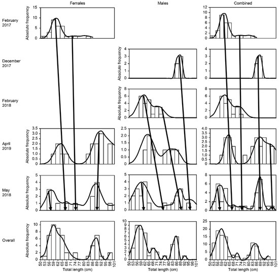
Figure 2.
Size frequency distribution (bars) and modal groups (lines) estimated for the bonnethead shark (Sphyrna tiburo) in the western Gulf of Mexico. (The months of the year are sorted sequentially without considering the year).
3.3. Fit of Growth Models
The VB1 model was not supported by any evidence (∆i > 10) in any of the three datasets (females, males, total) or according to either types of error assumed in the residuals (additive or multiplicative) (Table 3), while the model of Soriano et al. [40], with the variation in k and including L0 instead of t0, was the one selected for three datasets (females and total: S6; males: S4) with practically 100% of the evidence (wi) in its favor (females = 0.971, males = 1.00, total = 0.881) (Table 3 and Figure 3). In the total sample, S6 was selected because it was the only one that met the criterion of Δi < 2 (Table 3). This strong evidence in favor of the Soriano et al. [40] models selected with the L0 variation, estimated by the Gompertz model (S6) and by the same model (S4), in all three datasets (Figure 3) negated the need to use MMI.
Table 3.
Values of the maximum likelihood, the information criterion, and the specific weight of each candidate model, contributing to the description of growth patterns in females, males, and combined sexes of the bonnethead shark (Sphyrna tiburo) in the western Gulf of Mexico, under additive and multiplicative errors.
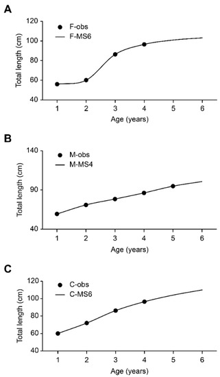
Figure 3.
Growth curves of females (A), males (B), and combined sexes (C) of Sphyrna tiburo from the western Gulf of Mexico. Dark filled circles are the observed values, and the lines are the estimated values. F−obs = observed values for females; F−S6 = model selected for females; M−obs = observed values for males; M−S6 = model selected for males; C−obs = observed values for combined sexes; and C−S6 = model selected for combined sexes.
Several models overestimated L∞ in females (VB2, G1, G2, J, and L1), in males (VB2, S5, S6, G1, and G2), and overall (VB2, S4, G1, G2, and J), and some also overestimated k in females (S1, S2, and S3), males (S1, S2, S3, and J), and overall (S1, S2, and S3) (Table 4). Several models underestimated k in females (G1, M2, and J), males (S6), and C (VB2). Based on the selected models (females and total: S6; males: S4), L0 was smaller in females (42.63 cm) than in males (44.37 cm) and the total sample (46.45 cm) (Table 4), and th occurred earlier in females (1.641 ± 0.061) than in males (3.48 ± 0.025), corresponding to Lth values of 53.34 cm (±0.919) and 81.35 cm (±0.025), respectively, while the overall th was 1.45 (±0.202) which was similar to the th in females, corresponding to a TL of 64.31 cm (Table 4).
Table 4.
Number of parameters (Φ) and values of the parameters estimated per model for females, males, and both sexes combined for the bonnethead shark (Sphyrna tiburo) in the western Gulf of Mexico.
In females, the AICc values were explained in a significant way (40%) by the number of parameters of the models (r2 = 0.399) (t = −3.4966, df = 1 and p < 0.05), but this hypothesis was not corroborated in males (r2 = 0.012; t = −0.3761, df = 1 and p > 0.05) or overall (r2 = 0.257, t = −2.0424, df = 1 and p > 0.05).
3.4. Differences in Total Lengths and Growth Curves
No significant differences were found between (a) the average sizes of females and males (t(1.98) = 0.329; df = 118; p > 0.05), (b) the values of ML, IC, and wi of the selected models in females (females(1, 5.317) = 3.60 × 10⁻⁷; p > 0.05), males (females(1, 5.317) = 3.10 × 10⁻⁶; p > 0.05) and C (females(1, 5.317) = 5.66 × 10⁻⁸; p > 0.05) (Table 3), or (c) the growth curves (χ2(9.488); df = 4; p > 0.05) of (i) the individual models selected from females (S6) and males (S4) (χ2 = 3.476), (ii) the individual selected and average models for females (χ2 = 0.1564), males (χ2 = 0.0641), and overall (χ2 = 0.0647), or (iii) the average model of females and males (χ2 = 4.0768) (Table 5). Therefore, based on a biological interpretation of the parameters, for both sexes, the S6 model, fit using the additive error in the Newton search algorithm [36], is adequate for representing the growth pattern of S. tiburo (Table 5).
Table 5.
Point estimates and confidence intervals of the growth parameters for the selected models and average models of the bonnethead shark (Sphyrna tiburo) in the western Gulf of Mexico.
4. Discussion
The objective of the present investigation was to describe the growth pattern of the bonnethead shark S. tiburo of western GM under the multimodel approach by fitting single−phase and biphasic models. In the three datasets (females, males, and both), the VB1 model did not present any statistical evidence in its favor (∆i > 10), and the model of Soriano et al. [40], with the second variant of the VB curve and including L0, was selected among the three datasets (females and total: S6; males: S4). L0 was similar in the three datasets (females = 42.63 cm, males = 44.37 cm, total = 46.45 cm). The age at which the transition between the two growth phases occurs in the selected model of Soriano et al. [40] was similar in females (1.641 ± 0.061) and total samples (1.449 ± 0.202) and lower than in males (3.48 ± 0.025). The model selected in C (S6) was sufficient to represent the growth pattern in S. tiburo.
To better characterize the growth of sharks, it is always recommended to use more than one growth function [19]. This study fit 13 growth models to frequency data of lengths with relative ages of S. tiburo. Multimodel inference was not applied because the selected models already provided enough evidence to choose them (wi = 0.90 or Δi < 2) [18]. The VB1 model did not provide enough statistical support to be selected, and the values of its parameters were not congruent with the biological reality of the species. Five studies that have described the growth pattern of S. tiburo: four in the GM [30,31,38,47], which were all on the western side of the state of Florida; and one for the Atlantic Ocean (east of Florida) [32]. The studies on the growth of this species in the GM have not applied the multimodel approach; only the one on the Atlantic population did. The studies carried out in the GM have only fit the VB1 model, and the study in the Atlantic used the multimodel approach to fit the classic growth models, VB, Gompertz, and logistic, finding that the best−fitting models were the Gompertz in females and VB in males.
Models with more than three parameters show better fits in large samples (n > 100) [48]. This was corroborated in this study, where the sample size was 104 specimens, and the best fitting model was Soriano et al. [40] model S6 with four parameters, while in males and females separately, the selected models were also those of Soriano et al. [40], S6 and S4 with four and five parameters, respectively. That is, they also had the greatest number of parameters. In some situations, several models (e.g., Gompertz and logistic) provide more precision than others (Von Bertalanffy and Schnute) in the estimation of the parameters in small samples (n ≤ 100) [48].
There is mounting evidence of biphasic growth in some species of sharks and rays, a group of large and a group of small organisms [17,49,50,51]. Braccini et al. [49] studied the growth pattern of the shark Squalus megalops in southeastern Australia by fitting five models whose base models were VB and Gompertz. In VB, the number of parameters 2 and 3 varied, and the second VB variant of the model of Soriano et al. [40] in its original version was applied (that is, without the recommendation of Cailliet et al. [19] to replace L0 by t0). The outcome was a choice of models and not a multimodel inference, favoring the model mentioned by Soriano et al. [40], both for females (wi = 0.54) and for males (wi = 95) because no model presented a value of Δi < 2. Mejía−Falla et al. [51] fit 10 monophasic and one biphasic growth model [40], using the model’s own variants and with different L0 values, to the age and size data of the round ray Urotrygon rogersi, which inhabits the Pacific coast of Colombia. In females and males, the model selected was the two−phase model of Soriano et al. [40]; in females it was variant 2 with five parameters, and in males it was the same model but with 4 parameters, where L0 was included according to Cailliet et al. [19] and its value was obtained from the literature. Biphasic growth in bony fishes has also been recently revealed. Aversa et al. [52] investigated the Argentine hake (Merluccius hubbsi) fishery and evaluated growth by fitting three models: VB, Gompertz, and the two−phase model, variant 2 of the Soriano et al. [40]. Like Braccini et al. [49] in their study of the Squalus megalops shark in southeastern Australia, the result was a choice of models and not a multimodel inference, thanks to the strong evidence in favor of the model of Soriano et al. [40] (wi = 0.99). In short, the studies on the growth pattern of elasmobranchs that have included the Soriano et al. [40] model among their set of candidate models have found that the observed data are better represented by this model than traditional models (Von Bertalanffy, Gompertz and Logistic).
The presence of these growth phases should be recognized by the models, but the models in use (VB, Gompertz, and logistic) usually do not record such growth phases (monophasic models) and tend to hide important ecological and evolutionary information [21]. This was the main hypothesis to be tested in this investigation in S. tiburo: the possible presence of two growth phases. In this study, seven single phase models (VB1, VB2, G1, G2, J, L1, and L2) and six biphasic models (all variants of [40]) with and without L0 competed. The model selected in females and overall was variant 2 of Soriano et al. [40] with the modification of L0 added by Caillet et al. [19], which was the one estimated with the Gompertz model and offered the best fit; in males, the model chosen was the same as in females but with the exception that L0 was estimated by the model of Soriano et al. [40] in its variant 2. The hypothesis guiding the study was corroborated: S. tiburo does present two growth phases. The possible causes of these growth phases are (a) energy investment in the reproductive process [22,23], (b) changes in habitat, (c) changes in diet, and (d) stressful situations [21,24,25].
The values of the growth parameters of S. tiburo estimated in this study are within the range of those reported in the literature [8,9,29,30,31,32,47,53,54,55,56]. In our study, the values of L∞ for females (106.45 cm) and males (122.18) were within the range of values reported in the literature: 80.40−139.80 cm and 70.30−125.08 cm, respectively (Table 6). The reported overall value (L∞ = 128.58 cm) is slightly higher than that estimated in the study based on the Castillo−Géniz [8] data for Playa Bagdad, Tamaulipas (127.10 cm). In the literature in some cases, L∞ was not estimated, and for comparative purposes in this study, it was calculated using the empirical method of Froese and Binohlan [57] (Table 6). Our value of k for males (0.22) was within the range of values reported in the literature (0.21−0.69 year−1) (Table 6), while those corresponding to females and overall were outside the estimated published limits (females = 0.16−0.37 year−1 and total = 0.17−0.24 year−1) (Table 6). Some studies have not reported k values, so we estimated it for comparative purposes using the empirical method of Munro and Pauly [58] and Moreau et al. [59] (Table 6).
Table 6.
Growth parameters (L∞, k, and L0) of the bonnethead shark Sphyrna tiburo reported in the literature.
The parameter th, according to the literature, varies by the biological event to be represented, based on the species. In teleosts, as fit by Soriano et al. [40], this parameter corresponds to a change in diet, mainly from juvenile to adult, while Araya and Cubillos [17] point out that th represents the age of onset of gonadal maturity. These authors found a significant linear relationship (r2 = 0.6797) between Lth and the size at gonadic maturity in sharks. Minte−Vera et al. [60] define the model of Soriano et al. [40] as that which includes two sequential VB model−type curves, whose point where the phases intersect corresponds to the beginning of reproductive maturity. In the case of the ray Urotrygon rogersi, this is not the case: Mejía−Falla et al. [51] fit the model of Soriano et al. [40] with the second variant of the VB curve to age and size data of U. rogersi, an endemic species of the Pacific coast of Colombia, indicating that th does not correspond to the size at reproductive maturity, but more likely to the size at fecundity.
In this study, th in females (1.64 years, equivalent to Lth = 53.34 cm) and both sexes (1.45 years, equivalent to Lth = 64.31 cm) would correspond more to the change in diet between the juvenile and adult stages, while in males (3.48 years, equivalent to Lth = 81.35 cm) it would correspond more to the size at the beginning of reproductive maturity. Kroetz et al. [61] point out that in this species, growth may decelerate because the organisms undergo a dietary change when transitioning from the juvenile phase to the adult phase; and Bethea et al. [62] managed to measure this change through the relative importance index (RII). They found that in the juvenile phase (1 year old), the dietary trend is to consume plant material (RII = 62.1), while the adult diet is composed mainly of crustaceans (RII = 73.1). As for reproductive maturity, the females matured between 85 and 90 cm and 80 and 85 cm in Tampa Bay and Florida Bay in the state of Florida [14], and in the GM, its size ranged from 77 to 91.2 cm [9,31,32,59]; in males, reproductive maturity occurs between 63.6 and 83 cm [31,32,59] in the GM; and in the overall population, Lombardi−Carlson [47] identified a reproductive maturity size of 77 cm over the combined areas of the state of Florida (northeast Florida, Tampa Bay, and Florida Bay) for the combined sexes. It is likely that this sexual dimorphism in the diet−change size and the reproductive−maturity size is because females (both juveniles and mature) inhabit estuarine waters, and males (juveniles and adults) mainly occur in coastal waters [63]. In this study, th occurred first in females (th = 1.64 years; Lth = 53.34 cm) and then in males (th = 3.48 years; Lth = 81.35 cm). Considering the reproductive−maturity size of females reported in the literature (80−90 cm) and assuming that in males the value of th (3.48 years; Lth = 81.35 cm) obtained in this study represents the size at reproductive maturity, the order of size at reproductive maturity in females and males that we found coincides with Araya and Cubillos [17], who identified such a pattern in seven of 10 analyzed shark species. The same was found by Cortés [64] studying S. tiburo off the coast of Florida, where females became reproductively mature at ages (2−3 years) older than males (2 years) off the coast of Florida. The point values of L0 estimated in this study are similar to those recorded for the Bays of Florida in the western part and greater than those indicated for the Atlantic Ocean side of Florida, and for the coastal states of the GM (Veracruz, Tabasco, Campeche, and Yucatan) (Table 6). However, the point values and the ranges of values obtained in this study (females 37.56−47.70 cm, males 42.27−46.46 cm, total 46.43−46.48 cm) lie within the range of values reported by the literature for the GM (females 37.21−55.18, males 36.02−55.54) (Table 6). The values in Table 6 for the GM were not estimated directly by Lombardi−Carlson [47] but were calculated by Frazier et al. [32] for comparative purposes between the GM and the Atlantic Ocean and were established based on the furcal length. With the same algorithms derived by Frazier et al. [32], we converted L0 values into total lengths (Table 6). The differences in the lengths of the offspring at birth (L0) may be due mainly to environmental factors at the localities where the organisms live [65].
Our findings have important implications. The main contribution of this study is the confirmation of the hypothesis of the biphasic growth pattern of the S. tiburo stock located in the west GM. Now the challenge is to corroborate this hypothesis in the rest of the stock throughout the entire GM. To do this, it is advisable to fit two−phase growth models to the average age and size data reported in the literature for the coasts of Florida [30,31,32,38] and to include biphasic models in the sets of candidate models for future investigations on the growth pattern of this species in the southeastern GM. In this way, the hypothesis that this species follows a growth pattern that has no oscillations but rather is isometric and continuous over all ages (VB1 model) in all areas of the GM would be indirectly tested.
Choosing only the VB1 model a priori brings the risk of underestimating or overestimating parameters, ignoring the uncertainty associated with model selection and losing the advantages of fitting the data to a parsimonious model [66]. If this research had been carried out in the traditional way, where only the VB1 model is chosen a priori, biased results would have been obtained. An example is the estimation of longevity with the Fabens [67] model specific to sharks [(5(ln2))k−1]. Using the values of k (0.54 year−1) obtained by the VB1 model in this study would have resulted in a longevity of 6.42 years, while using the value of k (0.23 year−1) estimated by the S6 model for both sexes in this work resulted in a longevity of 15.36 years, which is less biased than the values reported by the literature (12 years) [13].
Carefully estimating L∞ and k is essential to accurately assessing parameters and the fishing management reference points of any stock. One of the core parameters in any fisheries assessment is natural mortality, and in the literature many methods are reported to estimate it, several of which require the parameters L∞ and k, among others. Kenchington [68] indicated 17 methods of estimating mortality in fishes in general that require the value of the parameter k, while Zhou et al. [69] indicated nine methods that use mortality and one that uses k directly to estimate biological reference points in teleosts and chondrichthyans.
This study confirms the latitudinal variation pattern of the maximum lengths (Lmax) observed and the values of the growth parameters (L∞ and k) of S. tiburo, proposed by Lombardi−Carlson et al. [31]. The values of Lmax, L∞, and k estimated in this study for females (98 cm, 105.6 cm, and 0.54 year−1, respectively) and males (94 cm, 122.18 cm, and 0.22 year−1, respectively) are closer to those provided by Lombardi−Carlson et al. [31] for Florida Bay, which is the southernmost part of Florida (females 100 cm, 93.9 ± 58, and 0.29 ± 0.09 year−1, respectively; males 85 cm, 85.8 ± 9.2, and 0.25 ± 0.12 year−1), than for those reported from the Tampa Bay and northwest Florida. Florida Bay is geographically located at ~24°50′ N, while the study area of this paper is the coast of the municipalities of San Fernando and Soto La Marina in the state of Tamaulipas, Mexico, located at ~24°50′ N and ~23°78′ N, respectively. Tampa Bay and the northwest region of Florida are located at 28°10′ N and 29°40′ N, respectively.
Small samples are common in S. tiburo growth studies (n ≈ 100). In growth research of S. tiburo, small samples are often obtained from both commercial fishing and scientific sampling. Parsons [29], in his study from July 1982 to December 1986, obtained samples of 144 (females = 96, males = 48) and 99 individuals (females = 45, males = 44) from Tampa Bay and Florida Bay, respectively; in northeastern Florida (San Andrés Bay System and an arm of the sea in San Andrés) Carlson and Parsons [30] observed 115 individuals (females = 65, males = 50) in the period from October 1992 to October 1995; and Lombardi−Carlson [47] from March 1998 to September 2000 obtained samples from 191 individuals (females = 99, males = 92) in northeast Florida, 164 individuals in Tampa Bay (females = 79, males = 84), and 145 organisms in Florida Bay (females = 76, males = 69). Castillo−Géniz [8], in a study aiming to determine the size structure of the species in Playa Bagdad, Tamaulipas, collected only 73 individuals over 12 consecutive months. This author reported that this species represents 14.66% of commercial fisheries in the GM and 0.71% in Playa Bagdad in the Municipality of Matamoros, Tamaulipas, leading to the suggestion that this species’ low contribution to local fisheries production prevented them from estimating the catch per unit effort. In this study, the sample size was 104 individuals collected discontinuously from September 2016 to April 2019 for reasons related to the abundance of the species.
5. Conclusions
In this study, the hypothesis of two phase growth of S. tiburo is confirmed for the first time, and the hypothesis of continuous growth (VB models) traditionally reported by the literature is discarded. In particular, this species grows through the increase in the growth rate as a function of age, rather than the infinite length, adjusting for length at birth. The VB1 model did not have any supporting evidence of fitting the data observed in the three datasets (females, males, and total), while the evidence supporting the model of Soriano et al. [27] (two−phase) was so strong (wi = 100%) that it was not necessary to apply the MMI to any of the three datasets.
Taking the traditional approach of choosing VB1 a priori in this study would have yielded biased results, probably reflected as overestimated k values, which in turn would have led to an underestimation of longevity compared to what was obtained in this study and to that reported by the literature. The TL where the two growth phases overlap in females and both sexes is highly similar to the TL described by the scientific literature, where a dietary change occurs between the juvenile and adult stages, while in males this transition coincides more with the TLs reported by other studies, when reproductive maturity begins.
Now the challenge is to corroborate this hypothesis of two phase growth in the entire fishing stock of S. tiburo throughout the GM, mainly in southeastern Mexico and on both coasts of Florida, with published data and future data, and to verify this finding in the stocks of the rest of the small coastal sharks of the GM.
Author Contributions
Conceptualization, J.H.R.-C. and S.E.O.-d.l.F.; Methodology, J.H.R.-C., S.E.O.-d.l.F., F.T.-T.; Software, J.H.R.-C., J.A.R.-O.; Formal analysis, J.H.R.-C., J.A.R.-d.L., F.T.-T.; Research, J.H.R.-C., S.E.O.-d.l.F., J.A.R.-d.L., J.A.R.-O., F.T.-T.; Resources, J.H.R.-C., F.C.C.-R., F.T.-T.; Data processing, J.H.R.-C., S.E.O.-d.l.F., J.A.R.-O.; Writing of the original draft of the manuscript, J.H.R.-C., S.E.O.-d.l.F.; Writing, reviewing, and editing, J.H.R.-C., S.E.O.-d.l.F., F.T.-T.; Proofreading, J.H.R.-C., S.E.O.-d.l.F., J.A.R.-d.L., F.C.C.-R., J.A.R.-O., F.T.-T.; Supervision, J.H.R.-C., S.E.O.-d.l.F., J.A.R.-d.L., F.C.C.-R.; Project management, J.H.R.-C., F.T.-T. All authors have read and accepted the published version of the manuscript.
Funding
This work presents some results of the research project HIM/2015/017/SSA.1207 “Effects of mindfulness training on psychological distress and quality of life of the family caregiver”, Main researcher: Filiberto Toledano−Toledano. The present research was funded with federal funds for health research and was approved by the Commissions of Research, Ethics and Biosafety [Comisiones de Investigación, Ética y Bioseguridad], Hospital Infantil de México Federico Gómez, National Institute of Health. The funding agency had no control over the design of the study; the collection, analysis and interpretation of the data; or the writing of the manuscript.
Institutional Review Board Statement
The study was conducted according to the guidelines of the Declaration of Helsinki and approved by the Commissions of Research, Ethics and Biosafety [Comisiones de Investigación, Ética y Bioseguridad], Hospital Infantil de México Federico Gómez National Institute of Health.
Informed Consent Statement
Informed consent was obtained from all subjects involved in the study.
Data Availability Statement
The datasets used during the current study are available from the corresponding author on reasonable request.
Acknowledgments
The authors S.E.O.-d.l.F. and J.H.R.-C. thank biologists Alejandra Hernández Antonio and Gabriela Cárdenas Carreón for their help with sampling and the shark fishermen of San Fernando and Soto La Marina in Tamaulipas, Mexico, for allowing us to collect specimen data from their catches.
Conflicts of Interest
The authors declare no conflict of interest.
References
- Richardson, J. The Fish. In Fauna Boreali-Americana; or the Zoology of the Northern Parts of British America; J. Murray: London, UK, 1836; Volume 3, pp. 74–97. [Google Scholar]
- Rodríguez−Castro, J.H.; Adame−Garza, J.A.; Olmeda-de la Fuente, S.E. La actividad pesquera en Tamaulipas, ejemplo nacional. CienciaUAT 2010, 4, 28–35. [Google Scholar]
- Linnaeus, C. Systema Naturae per Regna tria Naturae, Secundum Classes, Ordinus, Genera, Species, cum Characteribus, Differentiis, Synonymis, Locis, 10th ed.; Laurentii Salvii: Holmiae, Sweden, 1758; 824p. [Google Scholar]
- Cortés, E.; Neer, J. Updated Catches of Atlantic Sharks. SEDAR 11 LCS05/06−DW−16; National Marine Fisheries Service, Southeast Fisheries Science Center: Panama, FL, USA, 2005.
- Pérez−Jiménez, J.C.; Mendez−Loeza, I. The small−scale shark fisheries in the Southern Gulf of Mexico: Understanding their heterogeneity to improve their management. Fish. Res. 2015, 172, 96–104. [Google Scholar] [CrossRef]
- Poey, F. Memorias Sobre la Historia Natural de la isla de Cuba, Acompañadas de Sumarios Latinos y Extractos en Francés; Imprenta de Barcina: Habana, Cuba, 1860; Volume 2. [Google Scholar]
- Ranzani, C. Dispositio familiae Molarum in genera et in species. Novi Comment. Acad. Sci. Inst. Bononiensis 1839, 3, 63–82. [Google Scholar]
- Castillo−Géniz, J.L. Aspectos Biológico−Pesqueros de los Tiburones Que Habitan las Aguas del Golfo de México; Tesis de Maestría, Facultad de Ciencias, Universidad Nacional Autónoma de México: México City, México, 2001. [Google Scholar]
- Márquez−Farias, F.; Castillo−Géniz, J.L.; de la Cruz, M.C.R. Demography of the bonnethead shark, Sphyrna tiburo (Linnaeus, 1758), in the Southeastern Gulf of Mexico. Cienc. Mar. 1998, 24, 13–34. [Google Scholar] [CrossRef][Green Version]
- DOF. NORMA Oficial Mexicana NOM−029−PESC−2006, Pesca Responsable de Tiburones y Rayas. Especificaciones para su Aprovechamiento; Diario Oficial de la Federación: México City, México, 2007.
- Müller, J.; Henle, F.G.J. Systematische Beschreibung der Plagiostomen; Veit und Comp.: Berlín, Germany, 1839; pp. 1–200. [Google Scholar]
- SEDAR. Stock Assessment Report Small Coastal Shark Complex, Atlantic Sharpnose, Blacknose, Bonnethead, and Finetooth Shark. In SEDAR 13 Stock Assessment Report; SEDAR: Calgary, Alberta, 2013. [Google Scholar]
- Cortés, E.; Parsons, G.R. Comparative demography of two populations of the bonnethead shark (Sphyrna tiburo). Can. J. Fish. Aquat. Sci. 1996, 53, 709–718. [Google Scholar] [CrossRef]
- Parsons, G.R.; Hoffmayer, E.R. Seasonal changes in the distribution and relative abundance of the Atlantic sharpnose shark rhizoprionodon terraenovaein the North Central Gulf of Mexico. Copeia 2005, 914–920. [Google Scholar] [CrossRef]
- Arkhipkin, A.I.; Roa−Ureta, R. Identification of ontogenetic growth models for squid. Mar. Freshw. Res. 2005, 56, 371–386. [Google Scholar] [CrossRef]
- Katsanevakis, S.; Maravelias, C.D. Modelling fish growth: Multi−model inference as a better alternative to a priori using von Bertalanffy equation. Fish Fish. 2008, 9, 178–187. [Google Scholar] [CrossRef]
- Araya, M.; Cubillos, L.A. Evidence of two−phase growth in elasmobranchs. Environ. Biol. Fishes 2006, 77, 293–300. [Google Scholar] [CrossRef]
- Burnham, K.P.; Anderson, D.R. Model Selection and Multimodel Inference: A Practical Information−Theoretic Approach; Springer: New York, NY, USA, 2002. [Google Scholar]
- Cailliet, G.M.; Smith, W.D.; Mollet, H.F.; Goldman, K.J. Age and growth studies of chondrichthyan fishes: The need for consistency in terminology, verification, validation, and growth function fitting. Environ. Biol. Fishes 2006, 77, 211–228. [Google Scholar] [CrossRef]
- Paine, C.E.T.; Marthews, T.R.; Vogt, D.R.; Purves, D.; Rees, M.; Hector, A.; Turnbull, L.A. How to fit nonlinear plant growth models and calculate growth rates: An update for ecologists. Methods Ecol. Evolut. 2012, 3, 245–256. [Google Scholar] [CrossRef]
- Wilson, K.L.; Honsey, A.E.; Moe, B.; Venturelli, P. Growing the biphasic framework: Techniques and recommendations for fitting emerging growth models. Methods Ecol. Evol. 2017, 9, 822–833. [Google Scholar] [CrossRef]
- Day, T.; Taylor, P.D. Von Bertalanffy’s growth equation should not be used to model age and size at maturity. Am. Nat. 1997, 149, 381–393. [Google Scholar] [CrossRef]
- Lester, N.P.; Shuter, B.J.; Abrams, P.A. Interpreting the von Bertalanffy model of somatic growth in fishes: The cost of reproduction. Proc. Biol. Sci. 2004, 271, 1625–1631. [Google Scholar] [CrossRef]
- Paloheimo, J.E.; Dickie, L.M. Food and growth of fishes: I. A growth curve derived from experimental data. J. Fish. Res. Board Can. 1965, 22, 521–542. [Google Scholar] [CrossRef]
- Parker, R.R.; Larkin, P.A. A concept of growth in fishes. J. Fish. Res. Board Can. 1959, 16, 721–745. [Google Scholar] [CrossRef]
- Contreras−Reyes, J.E.; Wiff, R.; Soto, J.; Donovan, C.R.; Araya, M. Biphasic growth modelling in elasmobranchs based on asymmetric and heavy-tailed errors. Environ. Biol. Fish 2021, 104, 615–628. [Google Scholar] [CrossRef]
- Beverton, R.J.H.; Holt, S.J. On the Dynamics of Exploited Fish Populations; Fisheries Investment Series; U.K. Ministry of Agriculture and Fisheries: London, UK, 1957; Volume 19.
- Thompson, W.F.; Bell, F.H. Biological statistics of the Pacific halibut fishery. 2. Effect of changes in intensity upon total yield and yield per unit of gear. Rep. Int. Fish. Commn. 1934, 8, 49. [Google Scholar]
- Parsons, G.R. Geographic variation in reproduction between two populations of the bonnethead shark, Sphyrna tiburo. Environ. Biol. Fishes 1993, 38, 25–35. [Google Scholar] [CrossRef]
- Carlson, J.K.; Parsons, G.R. Age and growth of the bonnethead shark, Sphyrna tiburo, from Northwest Florida, with comments on clinal variation. Environ. Biol. Fishes 1997, 50, 331–341. [Google Scholar] [CrossRef]
- Lombardi−Carlson, L.A.; Cortés, E.; Parsons, G.R.; Manire, C.A. Latitudinal variation in life−history traits of bonnethead sharks, Sphyrna tiburo, (Carcharhiniformes: Sphyrnidae) from the Eastern Gulf of Mexico. Mar. Freshw. Res. 2003, 54, 875–883. [Google Scholar] [CrossRef]
- Frazier, B.S.; Driggers, W.B.; Adams, D.H.; Jones, C.M.; Loefer, J.K. Validated age, growth and maturity of the bonnethead Sphyrna tiburo in the Western North Atlantic ocean. J. Fish Biol. 2014, 85, 688–712. [Google Scholar] [CrossRef] [PubMed]
- Haddon, M. Modelling and Quantitative Methods in Fisheries; Chapman and Hall: New York, NY, USA, 2001. [Google Scholar]
- Montgomery, S.S.; Walsh, C.T.; Kesby, C.L.; Johnson, D.D. Studies on the Growth and Mortality of School Prawns; FRDC Project No 2001(/029); Industry and Investment NSW–Fisheries Final Report Series No. 119; Cronulla Fisheries Research Centre of Excellence: Cronulla, Australia, 2010. [Google Scholar]
- Aguirre−Villasenor, H.; Morales-Bojórquez, E.; Morán-Angulo, R.E.; Madrid-Vera, J.; Valdez-Pineda, M.C. Biological indicators for the Pacific sierra (Scomberomorus sierra) fishery in the southern Gulf of California, Mexico. Cienc. Mar. 2006, 32, 471–484. [Google Scholar] [CrossRef][Green Version]
- Neter, J.; Kutner, M.H.; Nachtschien, J.; Wasserman, W. Applied Linear Statistical Models; McGraw−Hill: New York, NY, USA, 1996. [Google Scholar]
- Sparre, P.; Venema, S.C. Introduction to Tropical Fish Stock Assessment, Part 1: Manual. In FAO Fisheries and Aquaculture Technical Paper 306/1, Rev. 2; FAO: Rome, Italy, 1998. [Google Scholar]
- Parsons, G.R. Age determination and growth of the bonnethead shark Sphyrna tiburo: A comparison of two populations. Mar. Biol. 1993, 117, 23–31. [Google Scholar] [CrossRef]
- von Bertalanffy, L. A Quantitative theory of organic growth (inquiries on growth laws. II). Hum. Biol. 1938, 10, 181–213. [Google Scholar]
- Soriano, M.; Moreau, J.; Hoenig, J.M.; Pauly, D. New functions for the analysis of two−phase growth of juvenile and adult fishes, with application to nile perch. Trans. Am. Fish. Soc. 1992, 121, 486–493. [Google Scholar] [CrossRef]
- Ricker, W.E. Growth rates and models. In Fish Physiology: Bioenergetics and Growth; Hoar, W.S., Randall, D.J., Brett, J.R., Eds.; Academic Press: New York, NY, USA, 1979; pp. 677–743. [Google Scholar]
- Grosjean, P. Growth Model of the Reared Sea Urchin Paracentrotus Lividus (Lamarck, 1816). Ph.D. Thesis, Faculte des Sciences Laboratoire de Biologie Marine, Universite Libre de Bruxelles, Bruxelles, Belgium, 2001. [Google Scholar]
- Ricker, W.E. Computation and interpretation of biological statistics of fish populations. Bull. Fish. Res. Board Can. 1975, 191, 1–382. [Google Scholar]
- Mollet, H.F.; Ezcurra, J.M.; O’Sullivan, J.B. Captive biology of the pelagic stingray, Dasyatis violacea (Bonaparte, 1832). Mar. Freshw. Res. 2002, 53, 531–541. [Google Scholar] [CrossRef]
- Akaike, H. Information theory as an extension of the maximum likelihood principle. In Proceedings of the 2nd International Symposium on Information Theory, Tsahkadsor, Armenia, 2–8 September 1971; Petrov, B.N., Csaki, F., Eds.; pp. 267–281. [Google Scholar]
- Zar, J. Biostatistical Analysis; Prentice Hall: Hoboken, NJ, USA, 2009. [Google Scholar]
- Lombardi−Carlson, L.A. Life History Traits of Bonnethead Sharks, Sphyrna tiburo, from the Eastern Gulf of Mexico; SEDAR 13−DW−24; SEDAR: North Charleston, SC, USA, 2007. [Google Scholar]
- Thorson, J.T.; Simpfendorfer, C.A. Gear selectivity and sample size effects on growth curve selection in shark age and growth studies. Fish. Res. 2009, 98, 75–84. [Google Scholar] [CrossRef]
- Braccini, J.M.; Gillanders, B.M.; Walker, T.I.; Tovar−Avila, J. Comparison of deterministic growth models fitted to length−at−age data of the piked spurdog (Squalus megalops) in South−Eastern Australia. Mar. Freshw. Res. 2007, 58, 24–33. [Google Scholar] [CrossRef]
- Tribuzio, C.; Kruse, G.; Fujioka, J. Age and growth of spiny dogfish (Squalus acanthias) in the Gulf of Alaska: Analysis of alternative growth models. Fish. Bull. 2010, 108, 119–135. [Google Scholar]
- Mejía−Falla, P.A.; Cortés, E.; Navia, A.F.; Zapata, F.A. Age and growth of the round stingray Urotrygon rogersi, a particularly fast−growing and short−lived elasmobranch. PLoS ONE 2014, 9, e96077. [Google Scholar] [CrossRef] [PubMed]
- Aversa, M.I.; Dans, S.L.; GarcÍA, N.A.; Crespo, E.A. Growth models fitted to Dipturus chilensis length−at−age−data support a two phase growth. Rev. Chil. Hist. Nat. 2011, 84, 33–49. [Google Scholar] [CrossRef]
- Hernández−Betancourt, S.; Serrano−Flores, F.; Chumba−Segura, L.; Sélem−Salas, C.I. Los Tiburones en la Costa Norte de Yucatán: Poblaciones Amenazadas por la Sobrepesca? 2020. Available online: chrome-extension://efaidnbmnnnibpcajpcglclefindmkaj/viewer.html?pdfurl=https%3A%2F%2Fwww.ccba.uady.mx%2Fbioagro%2FV4N2%2FV4N2.pdf&clen=1738846&chunk=true (accessed on 11 February 2022).
- González−de Acevedo, M. Reproductive Biology of the Bonnethead (Sphyrna tiburo) from the Southeastern U.S. Atlantic Coast. Master’s Thesis, University of North Florida, Jacksonville, FL, USA, 2014. [Google Scholar]
- García−Alvarez, M.A. Uso de Recursos Tróficos por Rhizoprionodon terraenovae y Sphyrna tiburo, en el Sureste del Golfo de México. Master´s Thesis, Universidad Veracruzana, Veracrúz, México, 2014. [Google Scholar]
- Palacios−Hernández, D.; Castillo−Géniz, J.L.; Méndez−Loeza, I.; Pérez−Jiménez, J.C. Temporal and latitudinal comparisons of reproductive parameters in a heavily exploited shark, the bonnethead, Sphyrna tiburo (L. 1758), in the Southern Gulf of Mexico. J. Fish Biol. 2020, 97, 100–112. [Google Scholar] [CrossRef] [PubMed]
- Froese, R.; Binohlan, C. Empirical relationships to estimate asymptotic length, length at first maturity and length at maximum yield per recruit in fishes, with a simple method to evaluate length frequency data. J. Fish Biol. 2000, 56, 758–773. [Google Scholar] [CrossRef]
- Munro, J.L.; Pauly, D. A simple method for comparing the growth of fishes and invertebrates. Fishbyte 1983, 1, 5–6. [Google Scholar]
- Moreau, J.; Bambino, C.; Pauly, D. Indices of overall fish growth performance of 100 Tilapia (Cichlidae) populations. In The First Asian Fisheries Forum; Maclean, J.L., Dizon, L.B., Hosillos, L.V., Eds.; Asian Fisheries Society: Manilla, Philippines, 1986; pp. 201–206. [Google Scholar]
- Minte-Vera, C.V.; Maunder, M.N.; Casselman, J.M.; Campana, S.E. Growth functions that incorporate the cost of reproduction. Fish. Res. 2016, 180, 31–44. [Google Scholar] [CrossRef]
- Kroetz, A.M.; Drymon, J.M.; Powers, S.P. Comparative dietary diversity and trophic ecology of two estuarine mesopredators. Estuaries Coasts 2017, 40, 1171–1182. [Google Scholar] [CrossRef]
- Bethea, D.M.; Hale, L.; Carlson, J.K.; Cortés, E.; Manire, C.A.; Gelsleichter, J. Geographic and ontogenetic variation in the diet and daily ration of the bonnethead shark, Sphyrna tiburo, from the eastern Gulf of Mexico. Mar. Biol. 2007, 152, 1009–1020. [Google Scholar] [CrossRef]
- Ulrich, G.; Jones, C.; Driggers, W.B.I.; Drymon, M.; Oakley, D.; Riley, C. Habitat utilization, relative abundance and seasonality of sharks in the estuarine and near shore waters of South Carolina. Am. Fish. Soc. Symp. 2007, 50, 125–139. [Google Scholar]
- Cortés, E. Life history patterns and correlations in sharks. Rev. Fish. Sci. 2000, 8, 299–344. [Google Scholar] [CrossRef]
- Branstetter, S. Early life-history implications of selected carcharhinid and lamnoid sharks of the Northwest Atlantic. In Elasmobranchs as Living Resources: Advances in the Biology, Ecology, Systematics, and the Status of the Fisheries; Pratt, H.L., Gruber, S.H., Taniuchi, T., Eds.; NMFS: Maryland, MA, USA, 1990; pp. 17–28. [Google Scholar]
- Katsanevakis, S. Multi−model inference and model selection in Mexican fisheries. Cienc. Pesq. 2014, 22, 6–7. [Google Scholar]
- Fabens, A.J. Properties and fitting of the Von Bertalanffy growth curve. Growth 1965, 29, 265–289. [Google Scholar] [PubMed]
- Kenchington, T.J. Natural mortality estimators for information−limited fisheries. Fish Fish. 2013, 15, 533–562. [Google Scholar] [CrossRef]
- Zhou, S.; Yin, S.; Thorson, J.T.; Smith, A.D.M.; Fuller, M. Linking fishing mortality reference points to life history traits: An empirical study. Can. J. Fish. Aquat. Sci. 2012, 69, 1292–1301. [Google Scholar] [CrossRef]
Publisher’s Note: MDPI stays neutral with regard to jurisdictional claims in published maps and institutional affiliations. |
© 2022 by the authors. Licensee MDPI, Basel, Switzerland. This article is an open access article distributed under the terms and conditions of the Creative Commons Attribution (CC BY) license (https://creativecommons.org/licenses/by/4.0/).