Vortex Dynamics and Pinning in CaKFe₄As₄ Single Crystals from DC Magnetization Relaxation and AC Susceptibility

Abstract

Among various “families” of iron-based superconductors, the quite recently discovered AeAFe₄As₄ (where Ae is an alkali-earth metal and A is an alkali metal) has high critical current density, a very high upper critical field, and a low anisotropy, and has recently received much interest for the possibility of high magnetic field applications at the liquid hydrogen temperature. We have performed DC magnetization relaxation and frequency-dependent AC susceptibility measurements on high-quality single crystals of CaKFe₄As₄ with the aim of determining the pinning potential U*. The temperature dependence of U* displays a clear crossover between elastic creep and plastic creep. At temperatures around 27–28 K, U* has a very high value, up to 1200 K, resulting in an infinitesimally small probability of thermally activated flux jumps. From the dependence of the normalized pinning potential on irreversible magnetization, we have determined the creep exponents in the two creep regimes, which are in complete agreement with theoretical models. The estimation of the pinning potential from multifrequency AC susceptibility measurements was possible only near the critical temperature due to equipment limitations, and the resulting value is very close to the one that resulted from the magnetization relaxation data. Magnetic hysteresis loops revealed a second magnetization peak and very high values of the critical current density.

1. Introduction

In recent years, among many families of iron-based superconductors, the 122 system based on the AeFe₂As₂ “parent compound”, where Ae is an alkali-earth metal (Ca, Sr, Ba), became one of the most popular materials for fundamental studies and possible applications. The first reason for this was the possibility of growing quite large single crystals, which allowed a comprehensive investigation of their physical properties. It was revealed that they have a rather high critical temperature T_c up to 38 K [1], very high upper critical fields µ₀H_c2 (>70 T) [2,3] and low anisotropies γ (<2) [3], which make them strong candidates for high-field applications. Superconductivity in a non-superconducting “parent” compound AeFe₂As₂ is induced by alkali metal A substitution at Ae sites (A = Na, K, Rb, Cs). (Ae_1−xA_x)Fe₂As₂ has the same crystal structure symmetry as the parent compound, I4/mmm, because Ae and A randomly occupy equivalent sites. Actually, (Ae_1−xA_x)Fe₂As₂ can be viewed as solid solutions between AeFe₂As₂ and AFe₂As₂ compounds with the same crystallographic structure. However, if the difference in the ionic radius of Ae and A is too large, Ae and A cannot occupy equivalent sites in the unit cell, and a new “family” of IBSs appears [4], with a different structure: CaAFe₄As₄ (A = K, Rb, Cs) and SrAFe₄As₄ (A = Rb, Cs), noted AeA1144, in which there is an alternate stacking of the Ae and A layers across the Fe₂As₂ layer, changing the symmetry to P/4 mmm. The compounds are superconducting materials with critical temperatures T_c between 31 and 36 K. The most studied material in this new family is CaKFe₄As₄ (CaK1144). Considering potential high-field applications, the investigations of the types and strength of various effective pinning centers and of the critical current density and its dependence on temperature and field are of great importance. Planar defects, which are intergrowth of CaFe₂As₂ layers, with separation between them of about 50 nm, were revealed by high-resolution transmission electron microscopy (HRTEM). Due to their high density, it was suggested that those intergrowths are the strongest pinning centers for vortices along the ab-plane (when the applied field is parallel to the ab-plane) and they are responsible for the enhancement of J_c//ab at around 1 T [5]. More recently, HRTEM, combined with electron energy loss spectroscopy (EELS), showed that these planar defects consist of a network consisting of one or two layers of KFe₂As₂ spread over the periodically ordered KFe₂As₂, and of CaFe₂As₂ monolayers. In the same study, it was suggested that the regions with dark contrast are distributions of local strain due to the substitution of Ca by K in a unit cell [6]. In the above-mentioned studies on the excellent properties of CaKFe₄As₄ (CaK1144), the strength of the pinning centers was determined as a bulk pinning force from DC magnetic hysteresis loops. Here we investigated the mean pinning potential of the pinning centers in CaK1144 single crystals from magnetization relaxation measurements and frequency-dependent AC susceptibility studies.

2. Results

2.1. Magnetic Memory Effects

We first assessed the quality of the single crystals by checking the superconducting transition and the magnetic hysteresis loops, which all looked as expected. For reliable results from DC magnetic relaxation, it is important that the samples do not have magnetic history, i.e., there is no difference in the magnetic response for the three cooling protocols: zero-field cooling (ZFC), field-cooling (FC), and, respectively, field-cooling and measurement taken upon warming up (FCW). Figure 1 shows the temperature dependencies of the in-phase (real) and out-of-phase (imaginary) third harmonic susceptibility response, which is the most sensitive to discern between different vortex dynamics [7].

Figure 1 reveals that the third harmonic susceptibility response of the sample does not depend on the cooling regime, meaning it is a single crystal with excellent superconducting properties. In many other iron-based superconducting single crystals, there have been reported differences between the three cooling protocols, but the single crystal studied in this work displays absolutely no magnetic history effects.

2.2. Magnetization Relaxation

DC magnetization relaxation measurements can provide very useful information on the pinning potential (activation energy), the type of vortex creep (elastic or plastic), and the vortex creep exponent p that appears in the dependence of the pinning potential on the current density J [8]. We have performed a large number of such measurements at various temperatures.

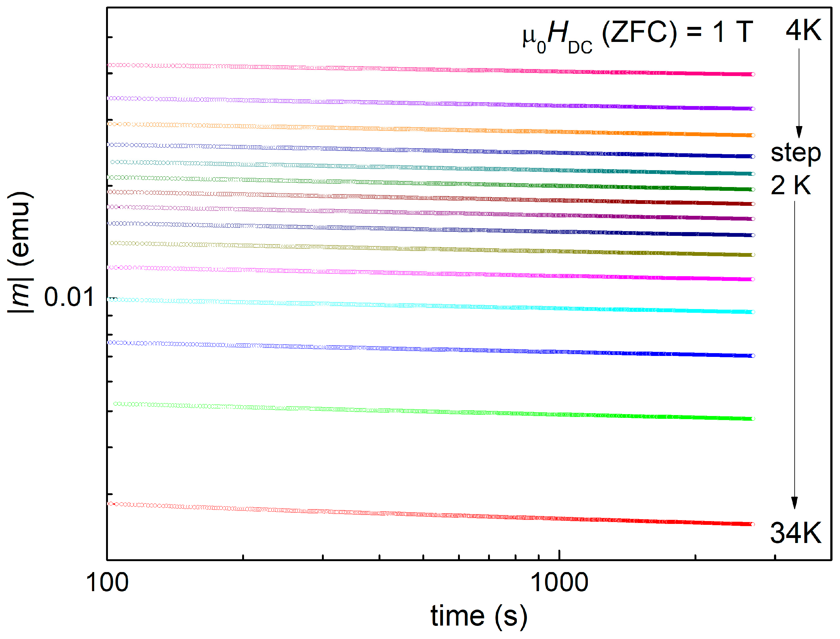
Figure 2 shows such magnetic relaxation measurements, |m|(t), at various temperatures and in a DC applied field, μ₀H_DC = 1 T, plotted in a double-logarithmic scale, which are clearly straight lines.

For relatively long measurement time t, the results of DC magnetization relaxation are consistent with thermally activated flux creep [8]. After the application of a DC external magnetic field H, and its subsequent removal, considering the parameterization of the pinning potential U [9] and the general vortex creep relation [10], the dependence of the pinning potential on temperature and time-dependent critical current U[J(t), T] is given by

U[J(t), T] = (U_c/p)[(J_c0/J)^p − 1] = Tln(t/t₀),

(1)

where U_c(T) is a characteristic pinning energy, J_c0(T) is the creep-free critical current density, and t₀ is the macroscopic time scale for creep (~10⁻⁶–1 s), which varies weakly with J(t). The theoretical models stated that the vortex creep exponent p is positive in the case of a collective (elastic) vortex creep regime, is negative for plastic creep regime, and depends mainly on the magnetic field H and the ratio J/J_c0. It should be noted that Equation (1) describes both elastic and plastic creep, while in a large number of publications, when dealing with (collective) elastic creep, creep exponent is expressed by μ, notation p being used only for the plastic creep. A hypothetical fit of the magnetization relaxation curves m_irr(t) ∝ J(t) using Equation (1) implies four parameters, clearly too many for acceptable conclusions, and usually results in values of the creep exponent p that are not consistent with any accepted model. The analysis is much more simplified in the cases in which, for a reasonably long measurement time, the double-logarithmic plots of m_irr(t) are straight lines, as is evident in Figure 2. In such cases, one can introduce and calculate a normalized relaxation rate S = −dln(|m_irr|)/dln(t) = −dln(J)/dln(t) and a normalized pinning potential U* = T/S [11]. In these conditions, for constant H and T, and if the overall J relaxation is not very high, which is the case of high-performance superconductors, p and t₀ can be considered constant, and the dependence of the normalized pinning potential on the current density is given by

U*(J) = U_c(J_c0/J)^p = U_c(|m₀|/|m_irr|)^p.

(2)

Following Equations (1) and (2), the normalized pinning potential is U* = U_c + pTln(t/t₀). For a moderate, window time for measurement and averaging t_w, we can consider that ln(t/t₀)~ln(t_w/t₀)~constant, and the normalized pinning potential is given by

U*(T) ~ U_c + pTln(t_w/t₀),

(3)

where U_c for elastic pinning is lower than the pinning energy for plastic pinning, when the plastic pinning structure can accommodate the vortices. Assuming that ln(U_c) and ln(J_c0) depend only weakly on temperature, which is the case for a relatively large T interval at fixed H_DC, the creep exponent p can be determined from the results of the magnetization relaxation measurements using Equation (2). For samples with strong pinning, as in our case, the data in the double-logarithmic plot (Figure 2) are very well described by a straight line with the slope being the normalized relaxation rate S = −dln(|m|)/dln(t). If the time of the measurement t_w is not too large, but is large in comparison with the macroscopic time for flux creep (~10⁻⁶–1 s), to stress the independence of the normalized relaxation rate on time, the normalized relation rate is often noted in the literature as S* = −Δln(|m|)/Δln(t). Using these considerations, we assumed that in the timeframe of our measurements (t₁ = 100 s < t < t_w = 2700 s), the slope is constant in time. In Figure 2, it is obvious that the experimental results are straight lines in the double-logarithmic scale. It can also be seen that for a fixed temperature, the time dependence of |m| ∝ J is very small in comparison with the change due to the variation of temperature, which is important for the determination of creep parameter p. 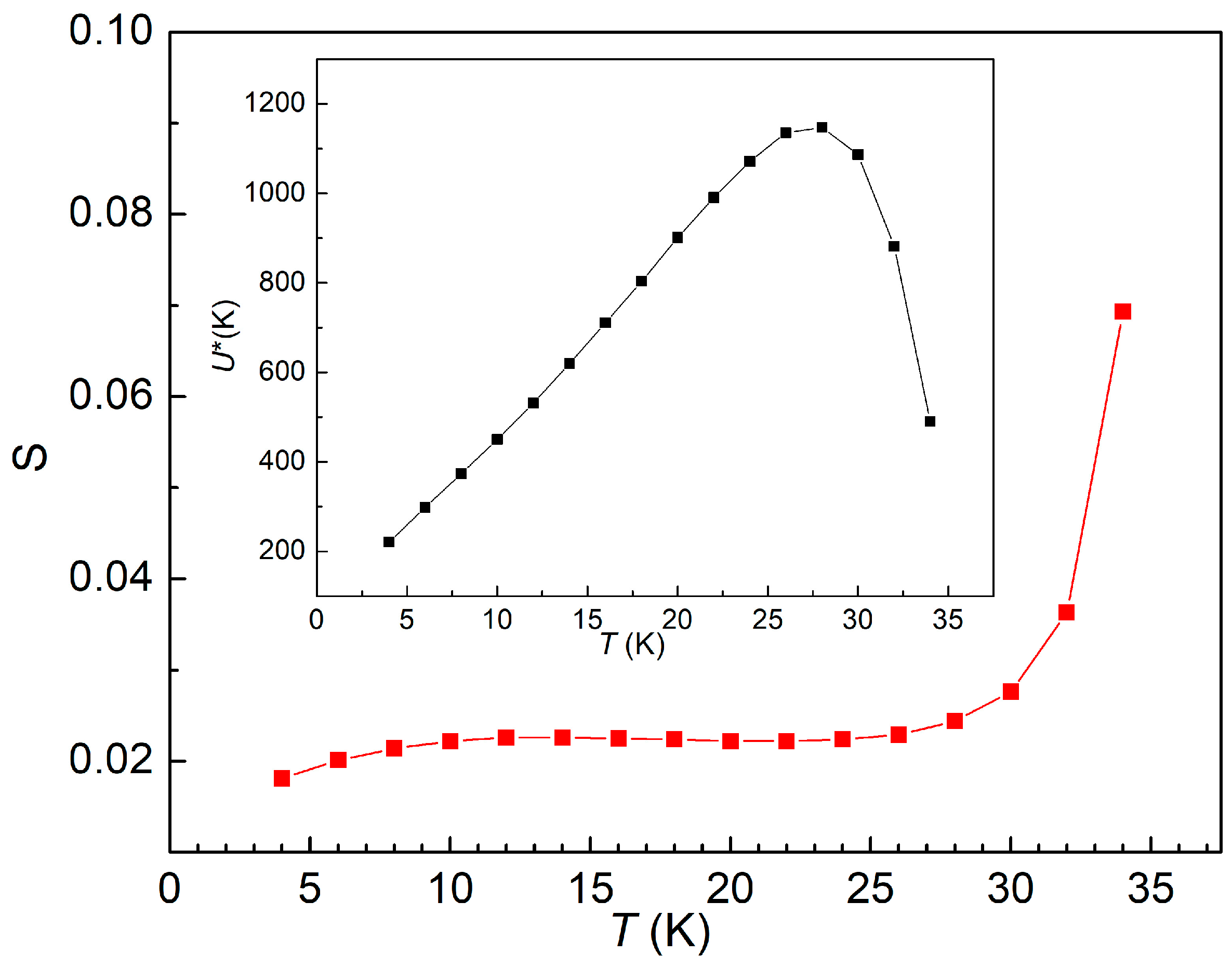From the measurements showed in Figure 2, we have determined for the DC field of 1 T the temperature dependence of the normalized relaxation rate S = −dln(|m|)/dln(t), as shown in Figure 3, and the normalized pinning potential, U* = T/S, as shown in the inset of Figure 3. Similar qualitative results were also obtained for other DC magnetic fields and reported elsewhere [12].

As can be seen in the inset of Figure 3, the temperature dependence of the normalized pinning potential U*(T) has a low-temperature region in which dU*(T)/dT is positive, characteristic of elastic creep, a high-temperature region in which dU*(T)/dT is negative, characteristic of plastic creep, and a maximum that separates the two regions, situated at about 28 K in 1 T. Equation (2), which gives the dependence of the pinning potential on the current density J ∝ |m| at a fixed temperature and magnetic field, allows the estimation of the creep exponent p, if, for not too long measurement time t_w, the decrease in |m| with time is small compared with the decrease in |m| with increasing temperature, which is the case for our sample (see Figure 2). With this approximation, we will consider a J_av(T,H) ∝ |m_av| (T,H) averaged over our measurement time. Averaging is made in the double-logarithmic scale, where the dependence is linear, as can be seen in Figure 2.

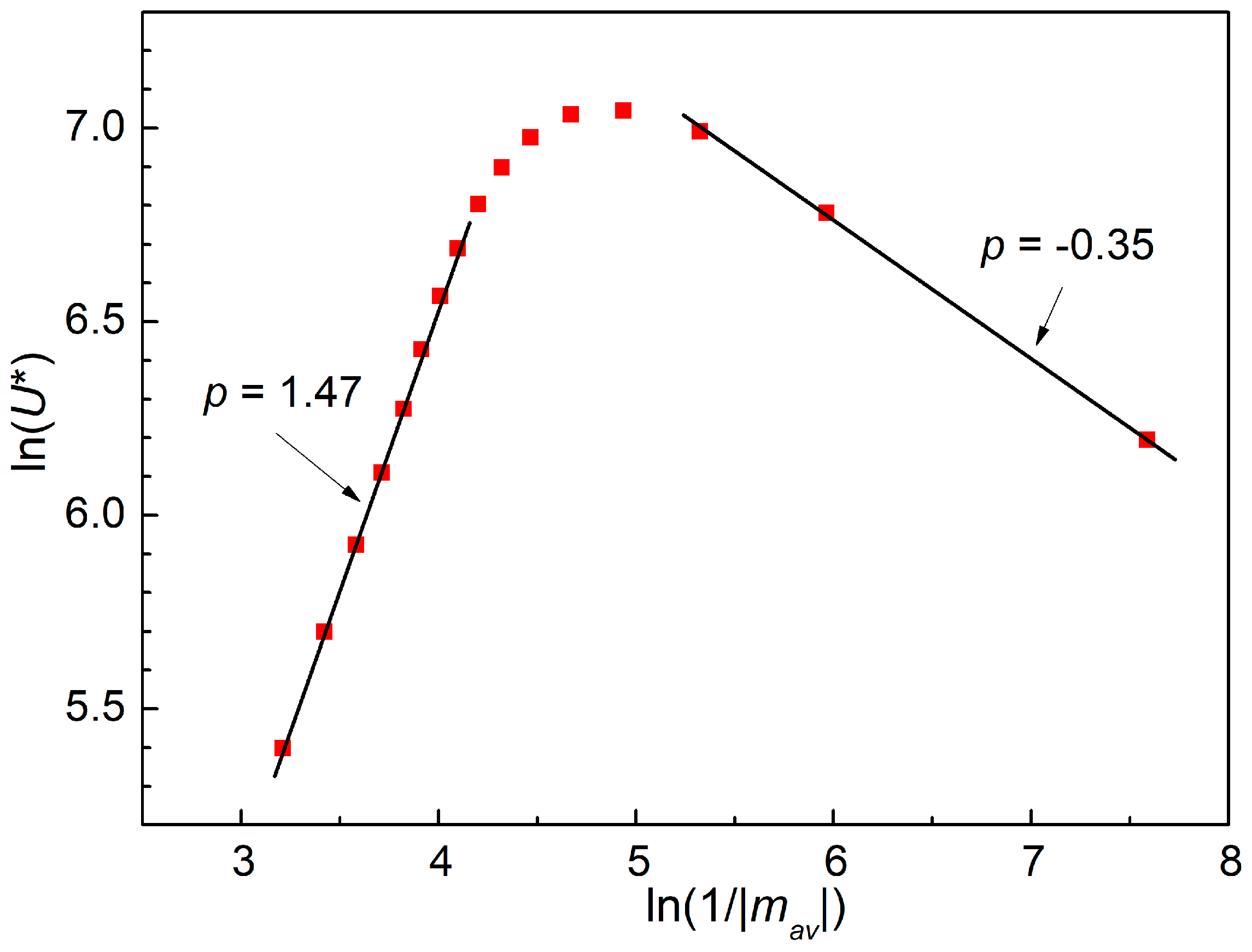
If we rewrite Equation (2) as ln(U*) = p[ln(1/|m_irr|) + const], the dependence of ln(U*) on ln(1/|m_av|) = ln(1/J_av) taken from the experimental data for each temperature, shown in Figure 4, allows the distinction between elastic creep and plastic creep, and the determination of the creep exponents.

In Figure 4, a rounded maximum of ln(U*) can be seen, which represents a crossover between elastic creep (left-hand side of the graph) and plastic creep (right-hand side). As can be seen from Equation (2), the slopes of the regions in Figure 4, where ln(U*) vs. ln(1/|m_av|) dependence is linear, represent the vortex creep exponent p, which is positive for elastic creep and negative for plastic creep.

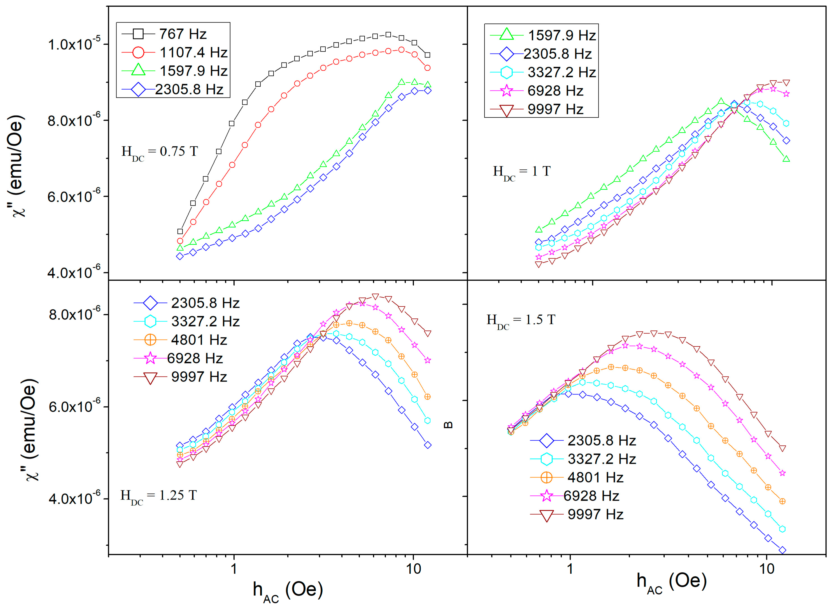
2.3. Frequency-Dependent AC Susceptibility

An alternative method of determining the pinning potential in superconductors is by employing the imaginary (out-of-phase) AC susceptibility response of the sample, χ″, as a function of AC field amplitude h_ac, for many frequencies of the AC field, at fixed temperatures T and fixed DC fields μ₀H_DC. At a fixed T, for several μ₀H_DC, χ″(h_ac) dependence may show a peak at h_ac = h*. The field h* actually represents the AC field of full penetration of the excitation in the center of the sample, which, in the critical state model, can be correlated with the critical current density of the material [13]. The positions of the above-mentioned peak depend on the frequency of the AC field excitation due to the different timescale for the vortices to leave the pinning centers. In the case of our CaK1144 single crystal, due to the very high critical current density, the experimental window in which the method is applicable was very close to the critical temperature. In fact, we could obtain useful results only at 35 K very close to the critical temperature, and for four applied DC fields, 0.75, 1, 1.25 and 1.5 T. The results are shown in Figure 5, the frequencies of the AC excitation fields being indicated in the figure. The selected measurement frequencies were equally distributed, in a logarithmic scale, between a minimum and a maximum one, hence the rather unusual values. It should be noted that the same frequency corresponds to the same symbol and color of the experimental data in any of the four panels of Figure 5.

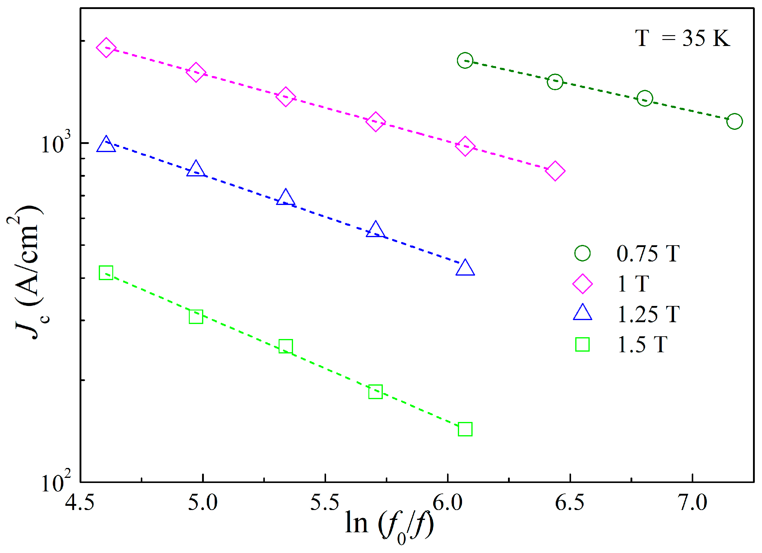
The thickness c of the crystal, 0.04 mm, is much smaller than the other two dimensions, so we could use the Brandt approach on the magnetic flux penetration [14], which gives the critical current density as a function of the position of the maximum h* in the χ″(h_ac) dependence as

J_c = h*/αc

(4)

where α ≈ 0.9 is a coefficient that depends slightly on the geometry (rectangle, square or disc), and c is the thickness, with h* in Oe, c in cm, and J_c in A/cm². By using Equation (4), from the h* values taken from the curves in Figure 5, we estimated the critical current densities at respective frequencies at 35 K and in the four μ₀H_DC mentioned above. Figure 6 presents the dependence of the critical current density J_c, shown in logarithmic scale, on ln(f₀/f), where f₀ is a macroscopic attempt frequency of about 10⁶ Hz. The shape of the experimental curves in Figure 6 indicates which model of pinning is suitable for our sample [15]: a downward curvature indicates an Anderson–Kim model of pinning with a linear dependence of the pinning potential on the probing current, an upward curvature indicates a collective pinning model with a power-law dependence of the pinning potential on the current, and a straight line in the double-logarithmic plot, as is the case of our measurements, is consistent with a logarithmic dependence of the pinning potential on the probing current density.

As was shown in [15], for the case of logarithmic dependence of the pinning potential on the current, the slope b of the straight lines in Figure 6 is related to the pinning potential U₀ = k_BT(1 + 1/b). From the slopes in Figure 6, we estimated the resulted values of U₀ in K (k_B = 1), for each μ₀H_DC: 260 ± 5 K (0.8 T), 210 ± 5 K (1 T),170 ± 5 K (1.25 T), and, respectively, 150 ± 5 K (1.5 T).

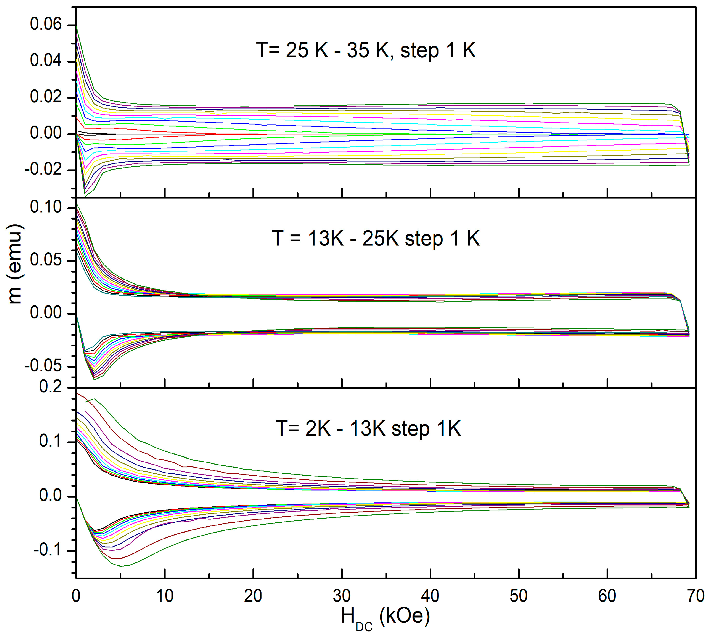
2.4. Magnetic Hysteresis Loops and Critical Current Density

Considering the high values of pinning potential in a wide temperature range, with values higher than 1000 K around the temperature of liquid hydrogen, it is also important to evaluate the critical current density J_c. For this purpose, we have performed magnetization hysteresis measurements to determine the field dependence of the irreversible magnetization, at various temperatures. Such measurements are shown in Figure 7, in which, for clarity, we present the results in three panels, with different scales for the magnetic moment m(H_DC, T), for the increasing and, respectively, decreasing applied magnetic field.

Several things can be seen in Figure 7. First, in increasing field branches at low fields, the Meissner screening is evident, followed by penetration of vortices, with diamagnetic response decreasing in absolute values. Then, at high temperatures (top panel) for fields higher than a certain value (irreversibility field, H_irr), magnetization is zero for both increasing (H)↑ and decreasing (H)↓ applied field. Also, a small Second Magnetization Peak (SMP) can be seen, which is a nonmonotonic variation of Δm(H) = m(H)↓ − m(H)↑. At an intermediate temperature, SMP is also very well seen, with a quite flat dependence of Δm(H) on the temperature. At low temperatures (bottom panel), SMP disappears, and Δm(H) has the normal decrease with increasing temperature and field.

Neglecting the low field data (for fields smaller than the lower critical field H_c1), from the Δm(H) data we can estimate the critical current density as a function of temperature and field, using the modified Bean critical state model [13]. With the dimensions of the rectangle (the face of the sample perpendicular to the magnetic field) l (length) and w (width), with l > w, and the sample dimension in the field direction d (thickness), the critical current density, in A/cm², is given by

$$J_c=\frac{60\Delta m}{w^{2}d\left(3l-w\right)},$$

(5)

with Δm(H) = m(H)↓ − m(H)↑ in emu, and all three dimensions in cm. If the sample is a square plate, i.e., l = w (which is the case of our sample), Equation (5) becomes

$$J_c=\frac{30\Delta m}{w^{3}d}$$

(6)

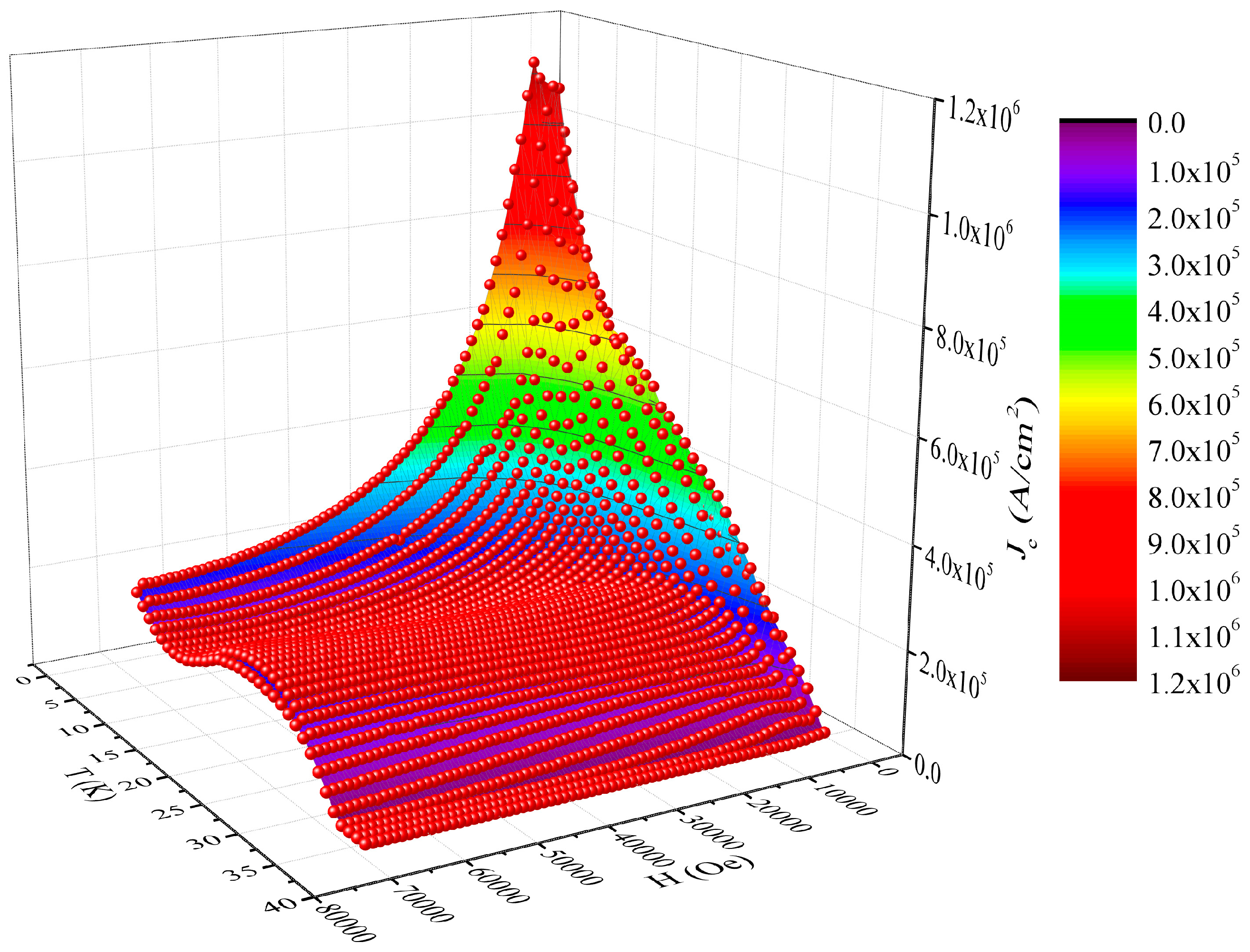
Using the data in Figure 7 and Equation (6), we evaluated the values of the critical current density as a function of field and temperature J_c (H, T), as shown in the 3-dimensional plot in Figure 8.

In Figure 8 we can clearly see the surface showing the second magnetization peak, as well as the quite high values of the critical current density, for temperatures not too close to the critical temperature, and for a wide range of applied magnetic fields. For temperatures around the temperature of liquid hydrogen (20 K), J_c is of the order of 10⁵ A/cm² even at the highest field of our measurements, which is quite important for future applications.

3. Discussion

A very important result from the magnetization relaxation measurements is the very high values of the normalized pinning potential U*, up to 1200 K at peak position, as can be seen in the inset of Figure 3. As the vortex creep is a thermally activated process, we can estimate the probability of a thermally activated flux jump (flux creep) out of the potential well associated with the pinning centers, which is proportional to exp(−U*/T), with U* in K (k_B = 1), which, for 1 T at about 27–28 K (U* ≈ 1200 K), is exp (−1200/27.5) = exp (−43.64) ≈ 10⁻¹⁹, an infinitesimally low value. For the lowest values of U* of 200 K at 4 K, liquid He temperature, the flux creep probability is exp (−200/4) = exp (−25) ≈ 10⁻¹¹. With these values, it is obvious that in CaK1144, at temperatures of practical interest, the dissipation due to thermally activated flux jump (flux creep) is negligible. Even at higher temperatures, in the plastic creep regime such probabilities are small, e.g., for U* ≈ 200 K at T ≈ 32 K, we have exp (−200/32) = exp (−6.25) ≈ 2 × 10⁻³.

Another important issue that resulted from magnetic relaxation measurement is the very clear crossover from elastic creep to plastic creep, with the creep exponents obtained for the two regions in very good agreement with theoretical predictions. Theoretical models for various collective (elastic) or plastic vortex creep regimes predict well-established values for vortex creep exponents [16]: 1/7 for single vortex collective creep, 3/2 or 5/2 [8] for small vortex bundle creep, and 7/9 for large vortex bundle creep. For high temperatures, the creep involves plastic vortex deformations, and p is negative (p = −0.5 for dislocation-mediated plastic creep) [17]. The smallest value for p is −1 (in the linear Anderson–Kim model [18]), while the largest one indicated by the elastic manifold theory in the small vortex bundle creep regime is 2.5 [8]. As can be seen in Figure 4, the creep exponent in the plastic creep region is p = −0.35, which is in good agreement with theoretical predictions p = −0.5 for dislocation-mediated plastic creep, while in the region of elastic creep, the value of the creep exponent, p = 1.47, is practically 3/2, as predicted, in the case of small vortex bundle elastic creep.

In the case of frequency-dependent AC susceptibility measurements, since CaK1144 has a very large critical current density and the maximum available h_ac provided by the equipment is 16 Oe, with this method, we had to probe a region in which critical current density is small enough to ensure that the corresponding h* (see Equation (4)) will not exceed 16 Oe. We could obtain the desired maxima in χ″(h_ac) only very close to the critical temperature in the plastic creep regime. For all four DC fields in which we obtained at least 4 curves, at various frequencies, that display a clear maximum, the frequency-dependent critical current is linear in a double-logarithmic plot, consistent with a logarithmic dependence of the pinning potential on the probing current as proposed by Zeldov et al., [19]. From the slopes of those dependences, we determined the values of the pinning potential.

In the case of DC magnetization relaxation measurements, we have estimated the normalized pinning potential in a large range of temperatures, between 4 K and critical temperature, covering the elastic creep regime, the plastic creep regime, and the crossover between the two regimes. The results of the AC susceptibility measurements allowed us to probe the vortex dynamics only in the plastic creep regime, very close to the critical temperature, where we were able to observe a maximum in χ″(h_ac). Extrapolating the U*(T) dependence from the magnetization relaxation in the insert of Figure 3 towards T = 35 K, one can estimate U*(35 K, 1 T) to be between 200 and 250 K, and a closer look at Figure 6b will show a value from AC susceptibility at the same temperature and DC field, U₀ (35 K, 1 T) ≈ 210 K, which is quite unexpected if one takes into account the much different timescale of the two types of measurements, 10³ s and 10⁻³ s, respectively. The probable explanation of this fact is that, very close to T_c, the viscosity of the plastic vortex matter is very small (practically becomes a vortex liquid), and the timescale of the low-viscosity plastic creep is less important.

From the magnetic hysteresis loops, we have observed a clear second magnetization peak at intermediate temperatures (around the temperature of liquid hydrogen) extended over a wide range of magnetic fields, as well as very high values of the critical current density in high magnetic fields in the region of SMP.

From the applications point of view, our results demonstrate the very high performance of this quite new superconducting material, especially for applications within the future hydrogen economy.

4. Materials and Methods

Single crystals of CaK1144 were grown at AIST Tsukuba, Japan using the FeAs-flux method. A precursor FeAs was prepared from Fe and As powders mixed in a 1:1 ratio and heated for 10 h at 900 °C in an evacuated quartz tube. Ca, K, and FeAs were mixed in a ratio of 1:1.1:10, which is a very large excess of FeAs. The mixture was placed in a zirconia crucible, which was sealed in a Ta container using an arc-welding chamber, then the Ta container was sealed in an evacuated quartz tube to protect Ta from oxidation, heated during 5 h to 650 °C and held at that temperature for 5 h for the preliminary sintering. The melting and crystallization were performed by heating to 1180 °C in 5 h, holding the temperature for another 5 h, cooling over 5 h to 1050 °C, and, finally, by very slowly cooling (0.025 °C/min) to 930 °C for 80 h. For this work, we have investigated single crystals having the shape of thin square discs, with dimensions a ≈ 1.2 mm, b ≈ 1.2 mm and c ≈ 0.04 mm.

We have used a commercial Quantum Design Magnetic Property Measurement System (MPMS) for the measurements of the DC magnetic hysteresis curves and magnetization relaxation. At temperatures well below T_c and above the field for the first full vortex penetration (in increasing H), or at any H in a decreasing field, the irreversible magnetic moment is considered to be the measured moment m. For the AC susceptibility measurements, we have used a commercial Quantum Design Physical Property Measurement System (PPMS) with the possibility of DC fields up to 14 T, in the ACMS set-up with frequencies up to 10 kHz and AC field amplitudes up to 16 Oe. In all the measurements presented in this paper, both DC and AC applied fields were perpendicular to the largest plane a–b of the single crystal, i.e., parallel to the c-axis.