Author Contributions
Conceptualization, M.P.P., S.B. and M.S.; methodology, M.P.P. and S.B.; software, M.P.P.; validation, M.P.P.; formal analysis, M.P.P.; investigation, M.P.P., S.B. and M.S.; data curation, M.P.P.; writing—original draft preparation, M.P.P.; writing—review and editing, M.P.P., S.B. and M.S.; visualization, M.P.P.; supervision, S.B. and M.S.; funding acquisition, S.B. and M.S. All authors have read and agreed to the published version of the manuscript.
Figure 1.
A 3D visualization of the simplified geometry. The detector planes are shown in blue, the container model in red and some generic objects representing the container content in green. In addition, an example of a trajectory of an air shower particle (gray line) with secondary particle production (yellow lines) is depicted.
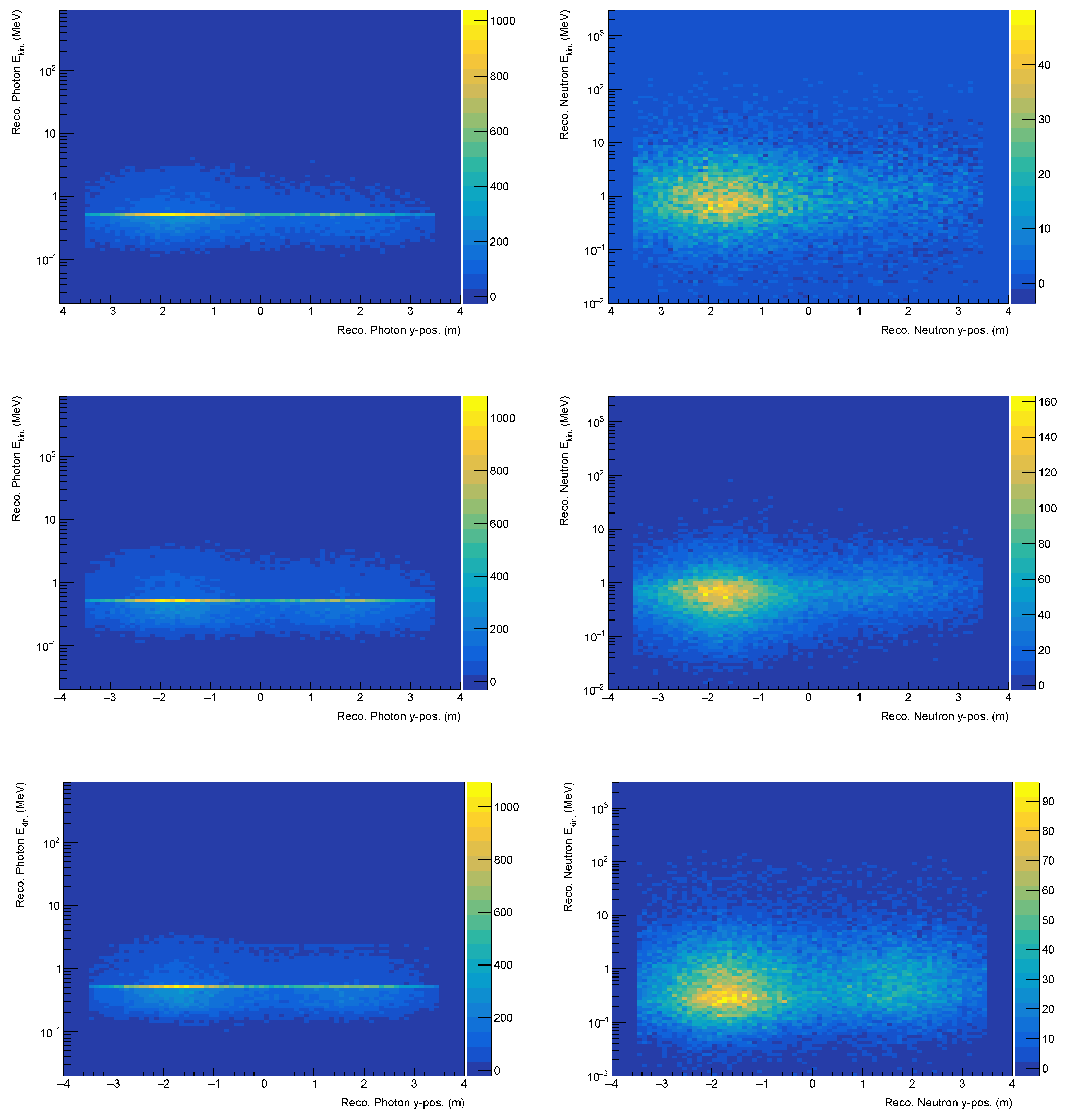
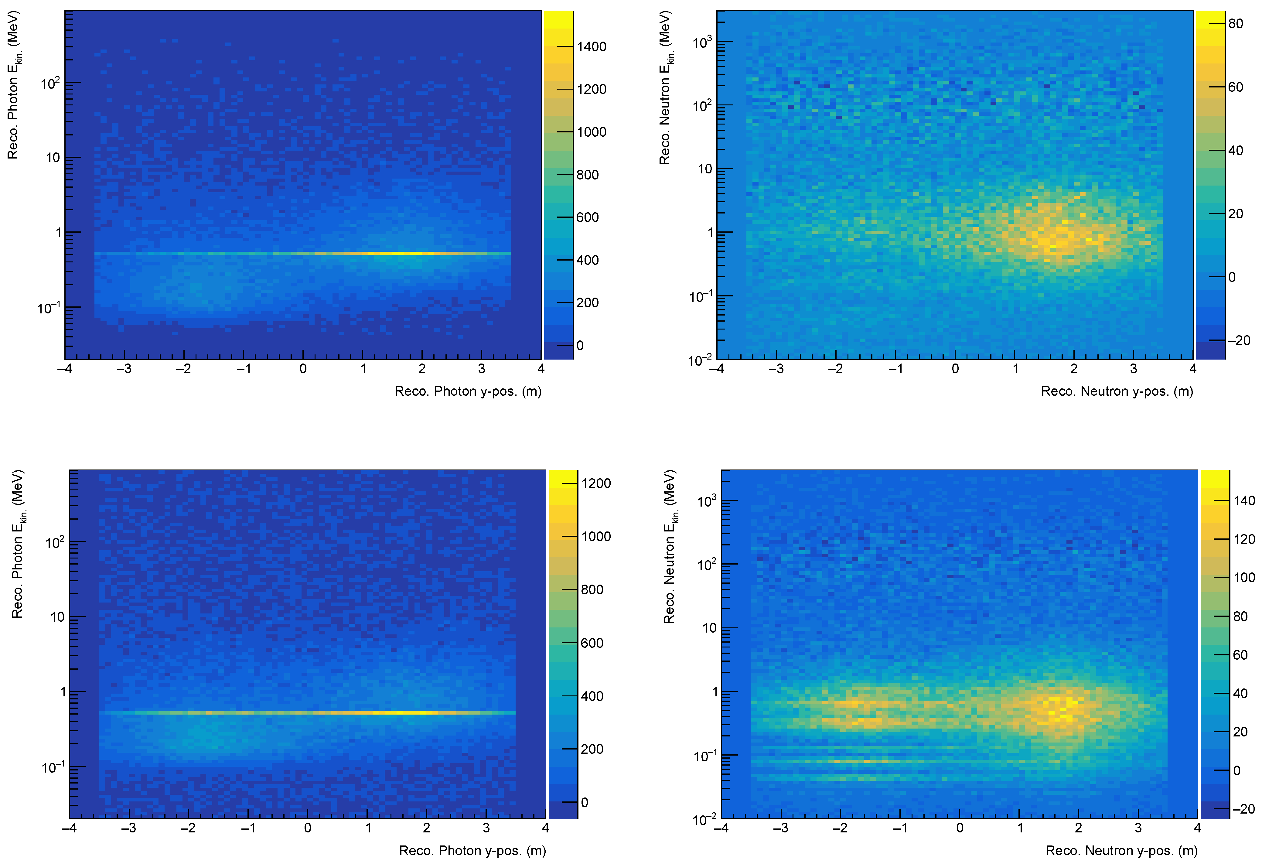
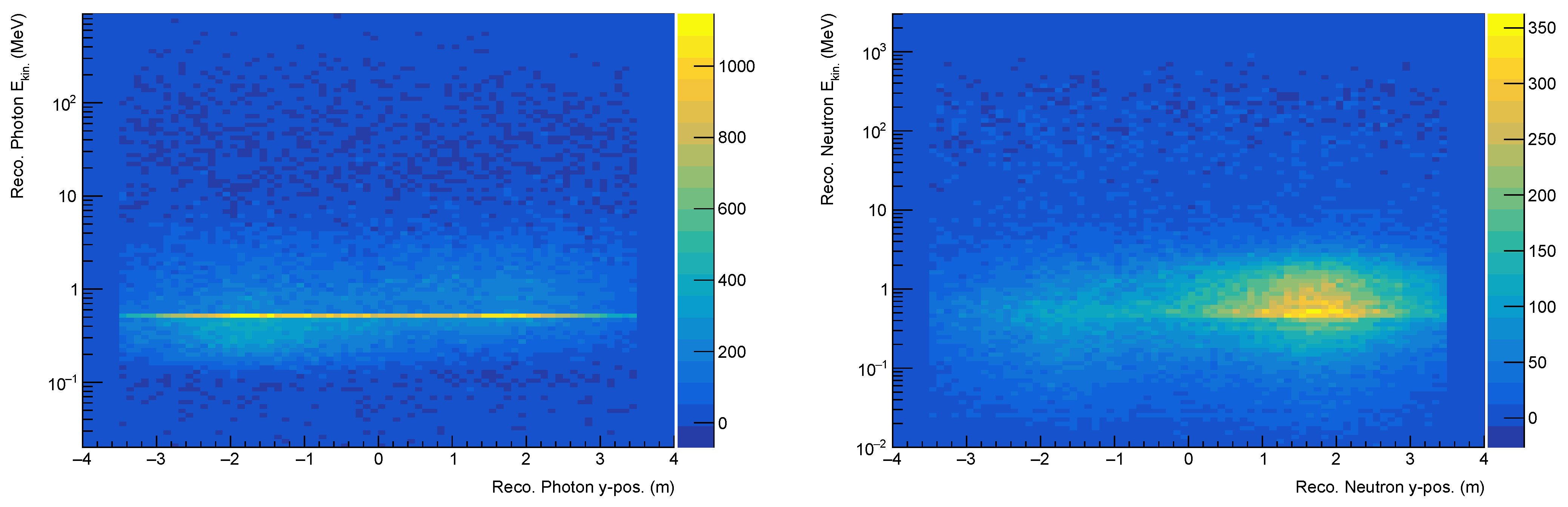
Figure 2.
The distribution of the kinetic energy as a function of the of the reconstructed photons (left column) and neutrons (right column) in the upper detector plane. The materials analyzed are Cesium (upper row), Tin (middle row) and Palladium (bottom row). The hits from the empty container are subtracted.
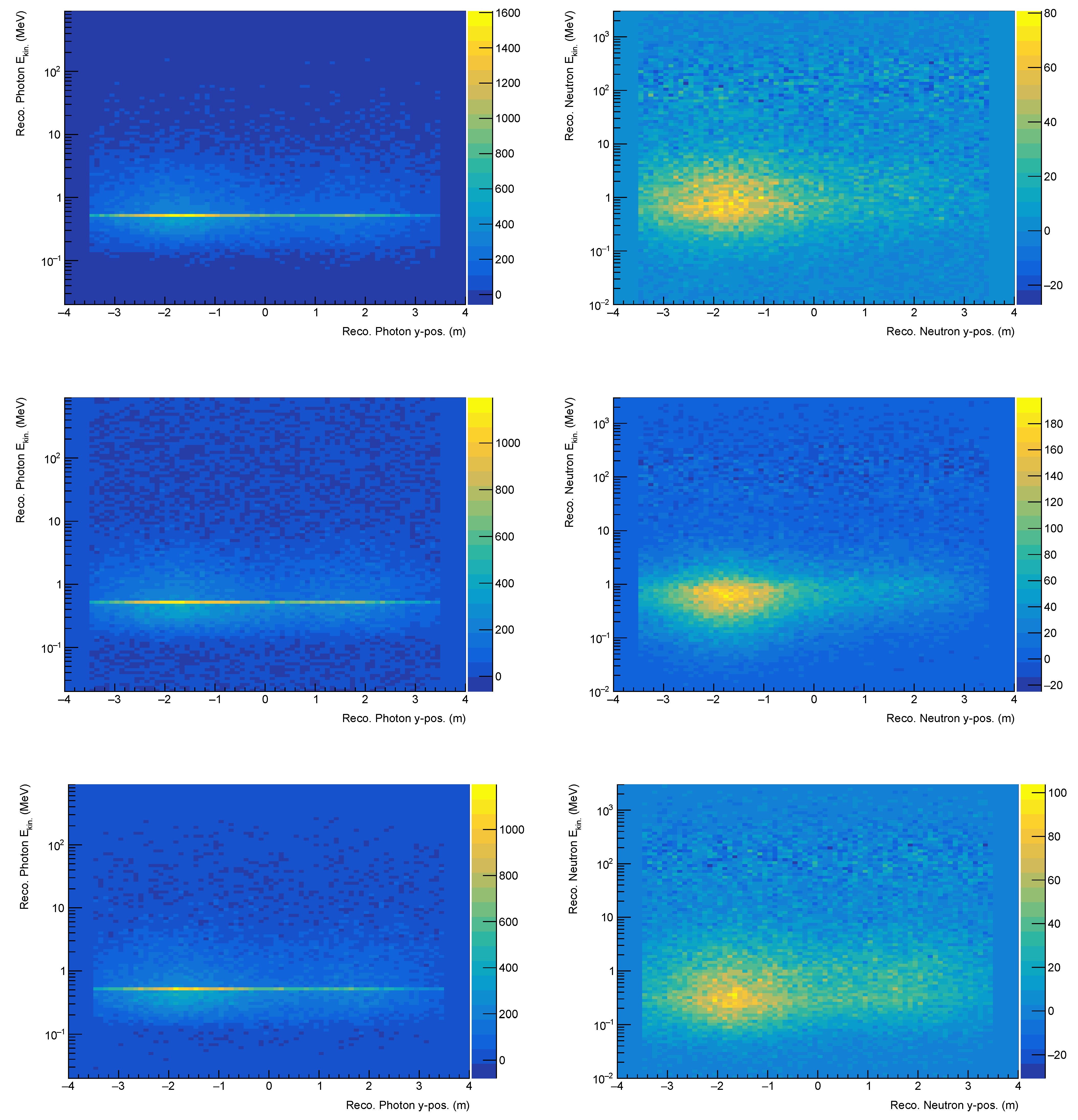
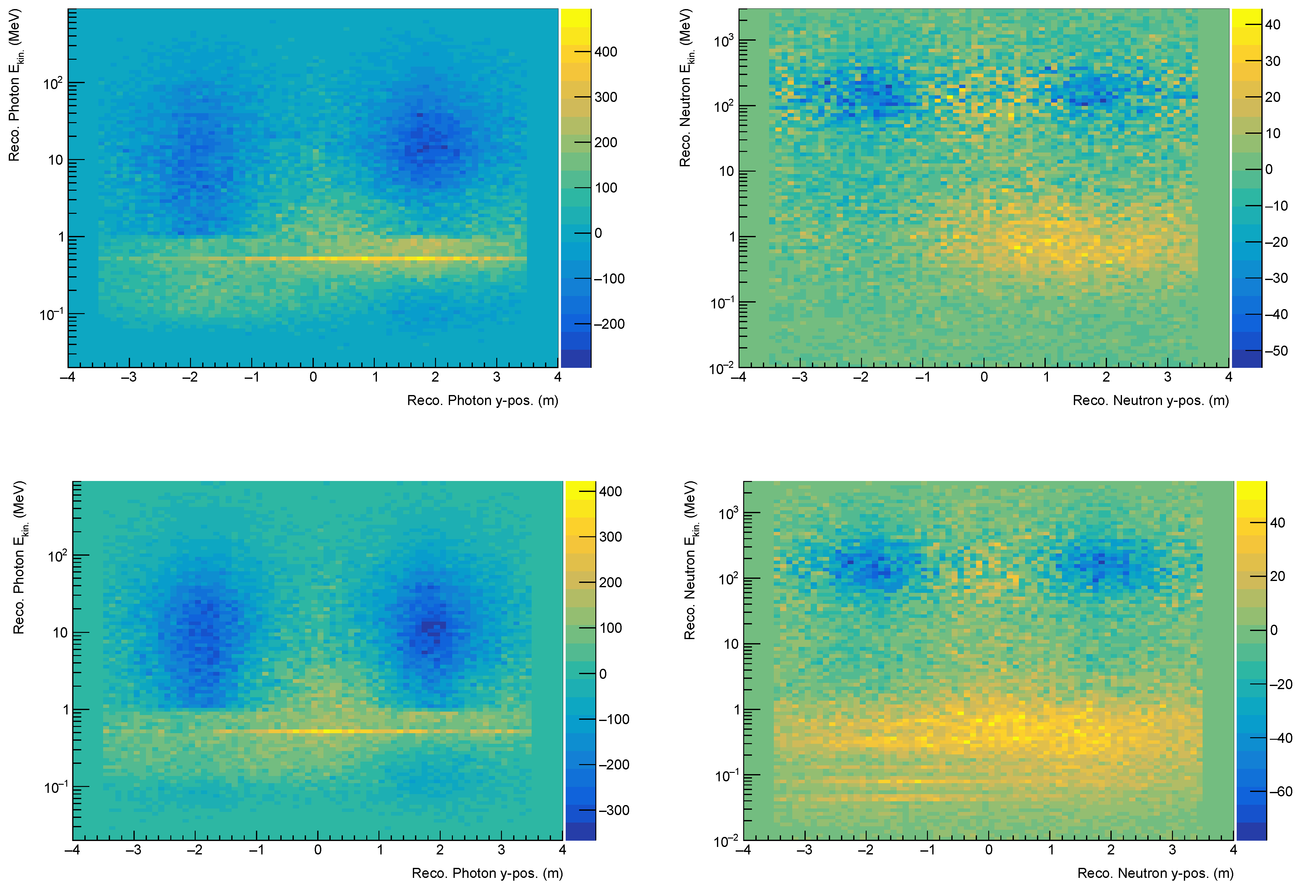
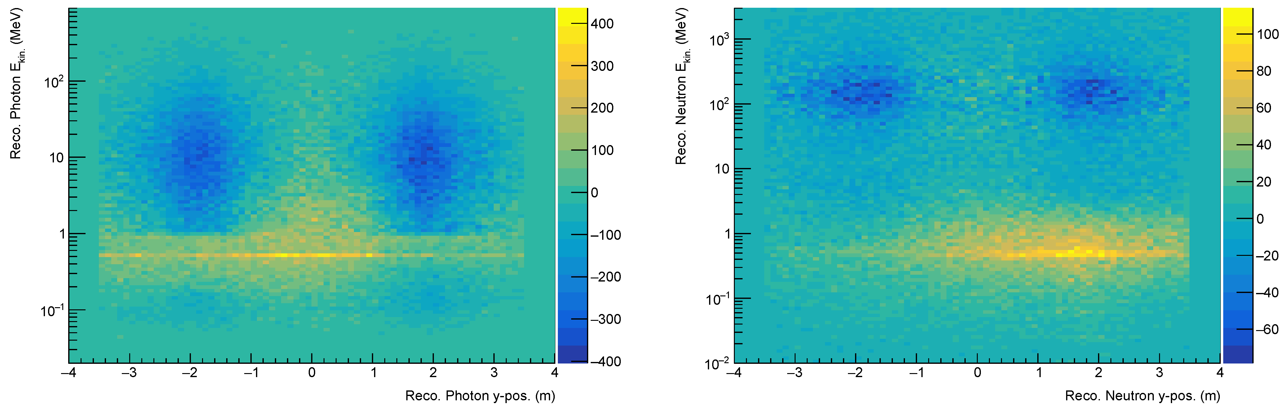
Figure 3.
The distribution of the kinetic energy as a function of the of the reconstructed photons (left column) and neutrons (right column) in the sidewise detector planes. The materials analyzed are Cesium (upper row), Tin (middle row) and Palladium (bottom row). The hits from the empty container are subtracted.
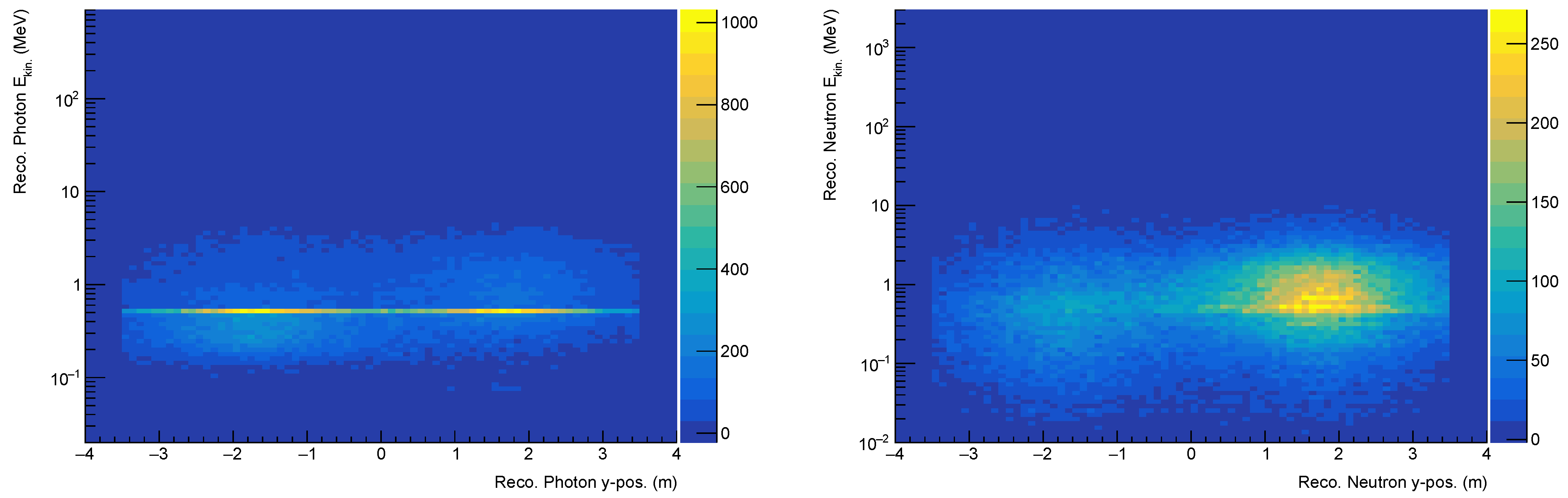
Figure 4.
The distribution of the kinetic energy as a function of the of the reconstructed photons (left column) and neutrons (right column) in the lower detector plane. The materials analyzed are Cesium (upper row), Tin (middle row) and Palladium (bottom row). The hits from the empty container are subtracted.
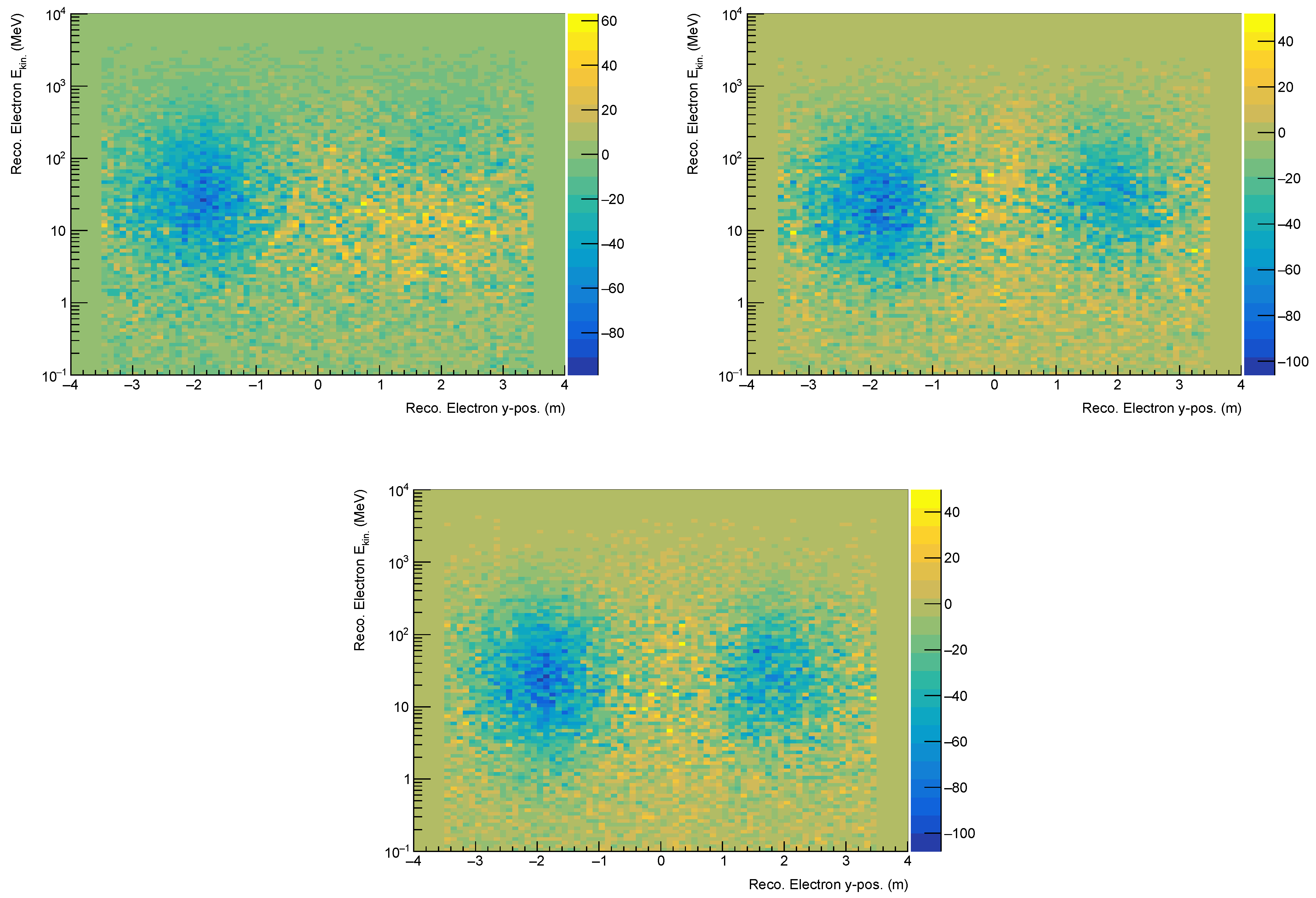
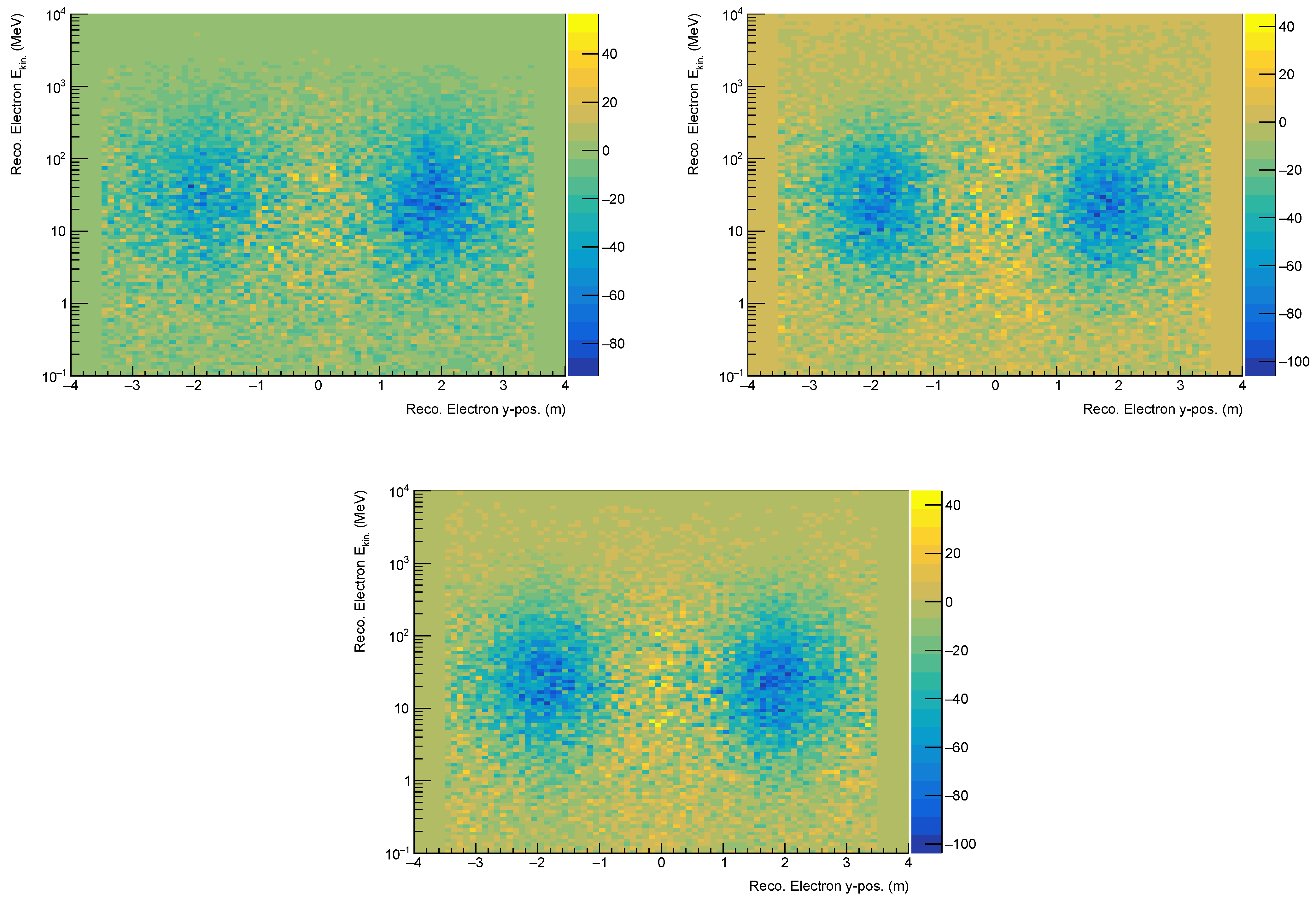
Figure 5.
The distribution of the kinetic energy as a function of the of the reconstructed electrons in the lower detector plane. The materials analyzed are Cesium (top left), Tin (top right) and Palladium (bottom). The hits from the empty container are subtracted.
Figure 5.
The distribution of the kinetic energy as a function of the of the reconstructed electrons in the lower detector plane. The materials analyzed are Cesium (top left), Tin (top right) and Palladium (bottom). The hits from the empty container are subtracted.
Figure 6.
The distribution of the kinetic energy as a function of the of the reconstructed photons (left column) and neutrons (right column) in the upper detector plane. The materials analyzed are Magnesium and Cesium (upper row), Chromium and Ytterbium (middle row), as well as Molybdenum and Lead (bottom row). The hits from the empty container are subtracted.
Figure 7.
The distribution of the kinetic energy as a function of the of the reconstructed photons (left column) and neutrons (right column) in the sidewise detector planes. The materials analyzed are Magnesium and Cesium (upper row), Chromium and Ytterbium (middle row), as well as Molybdenum and Lead (bottom row). The hits from the empty container are subtracted.
Figure 8.
The distribution of the kinetic energy as a function of the of the reconstructed photons (left column) and neutrons (right column) in the lower detector plane. The materials analyzed are Magnesium and Cesium (upper row), Chromium and Ytterbium (middle row), as well as Molybdenum and Lead (bottom row). The hits from the empty container are subtracted.
Figure 9.
The distribution of the kinetic energy as a function of the of the reconstructed electrons in the lower detector plane. The materials analyzed are Magnesium and Cesium (upper row), Chromium and Ytterbium (middle row), as well as Molybdenum and Lead (bottom row). The hits from the empty container are subtracted.
Figure 10.
A 2D visualization of the particle back-tracing process and the score assignment. A hit is shown as a solid dot and its projected trajectory with a dashed line. The total, non-zero voxel scores are shown in the corners of each voxel and are also represented by the color.
Figure 10.
A 2D visualization of the particle back-tracing process and the score assignment. A hit is shown as a solid dot and its projected trajectory with a dashed line. The total, non-zero voxel scores are shown in the corners of each voxel and are also represented by the color.
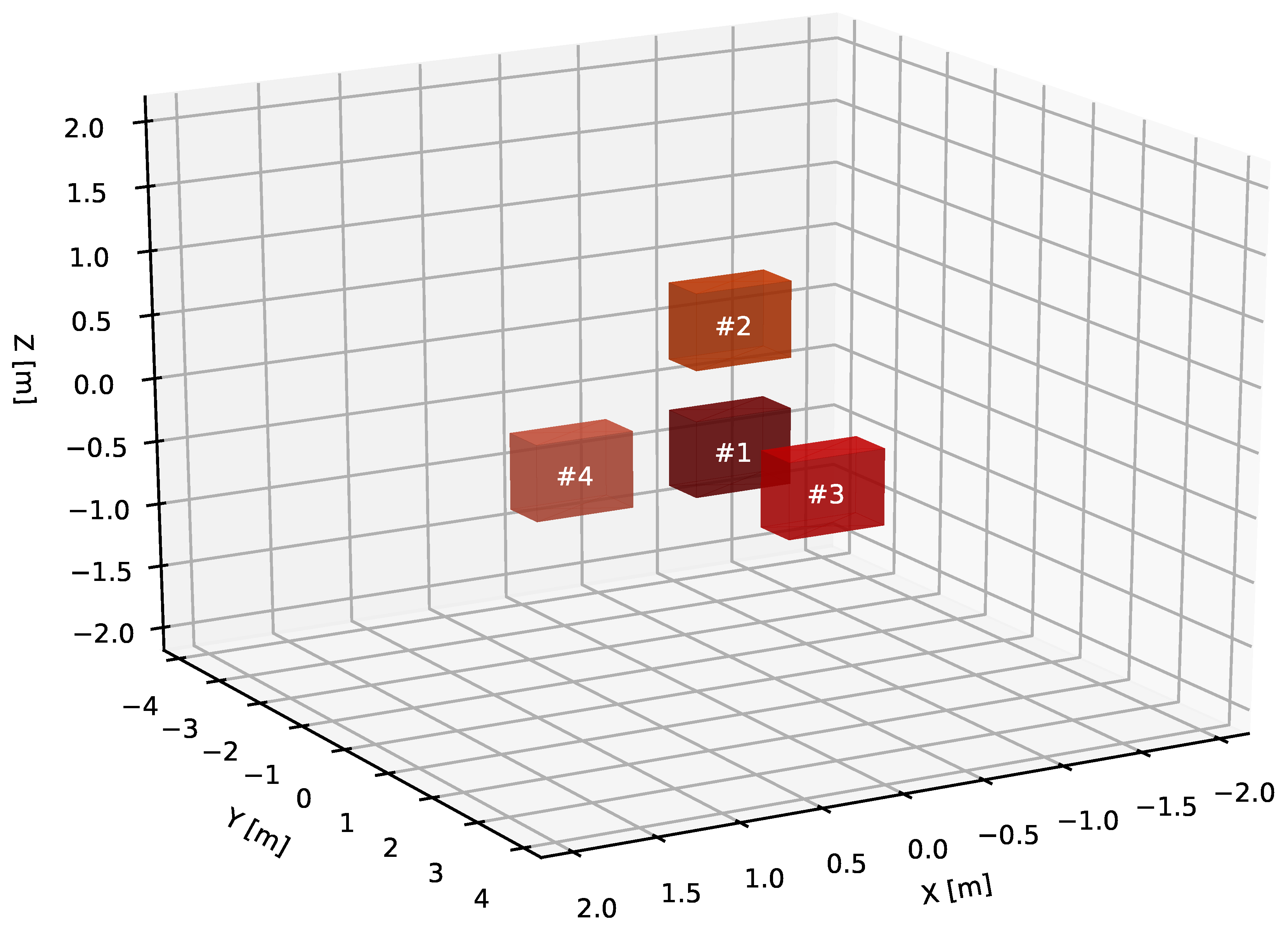
Figure 11.
A 3D visualization of the location of the four lead cubes in test scenario 3.
Figure 11.
A 3D visualization of the location of the four lead cubes in test scenario 3.
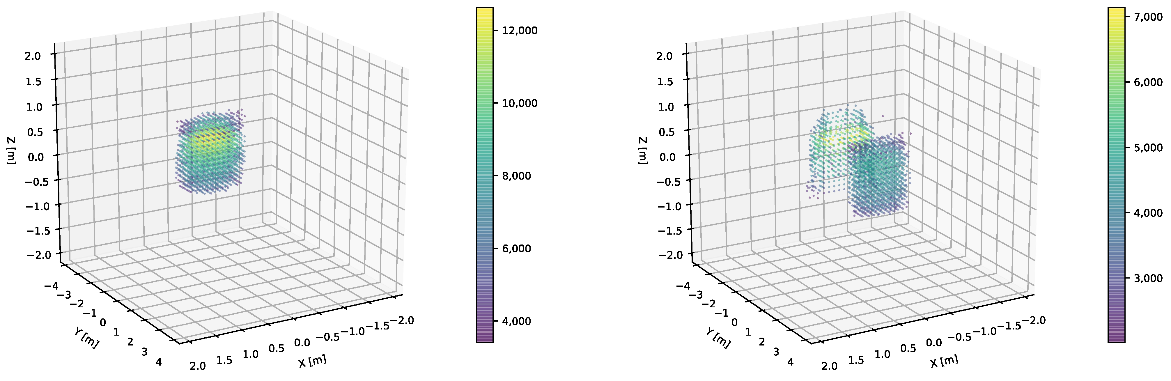
Figure 12.
The 3D voxel map of separate water and lead blocks reconstructed with the parameter set optimized for lead as shown in
Table 3 (
left) and water as shown in
Table 4 (
right). The color of the voxel point represents the combined voxel score
.
Figure 12.
The 3D voxel map of separate water and lead blocks reconstructed with the parameter set optimized for lead as shown in
Table 3 (
left) and water as shown in
Table 4 (
right). The color of the voxel point represents the combined voxel score
.
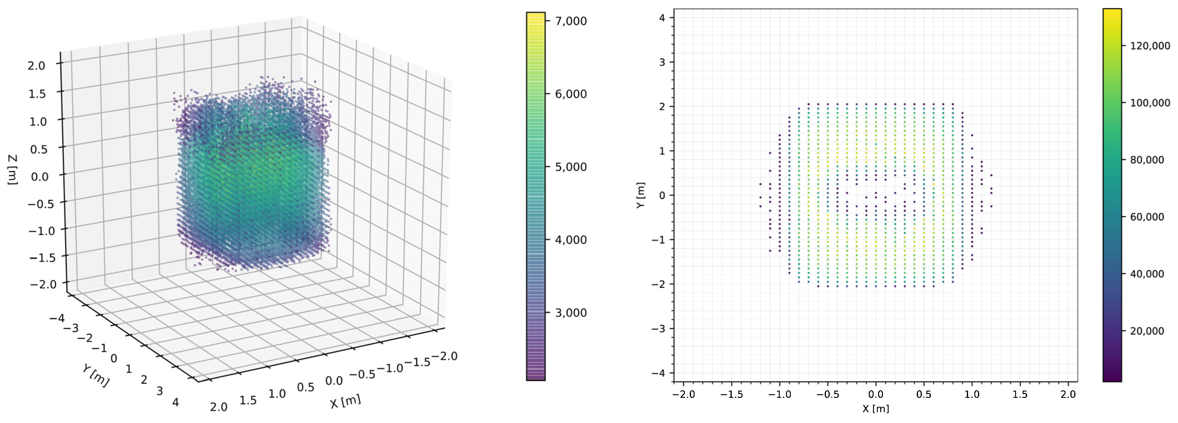
Figure 13.
The 3D voxel map of the lead block in the water basin (
left) and its 2D projection (
right) reconstructed with the parameter set optimized for lead block in water basin as shown in
Table 5. The color of the voxel point represents the combined voxel score
.
Figure 13.
The 3D voxel map of the lead block in the water basin (
left) and its 2D projection (
right) reconstructed with the parameter set optimized for lead block in water basin as shown in
Table 5. The color of the voxel point represents the combined voxel score
.
Figure 14.
The 3D voxel map of the lead block in the water basin (
left) and its 2D projection (
right) reconstructed with the parameter set optimized for water as shown in
Table 4. The color of the voxel point represents the combined voxel score
.
Figure 14.
The 3D voxel map of the lead block in the water basin (
left) and its 2D projection (
right) reconstructed with the parameter set optimized for water as shown in
Table 4. The color of the voxel point represents the combined voxel score
.
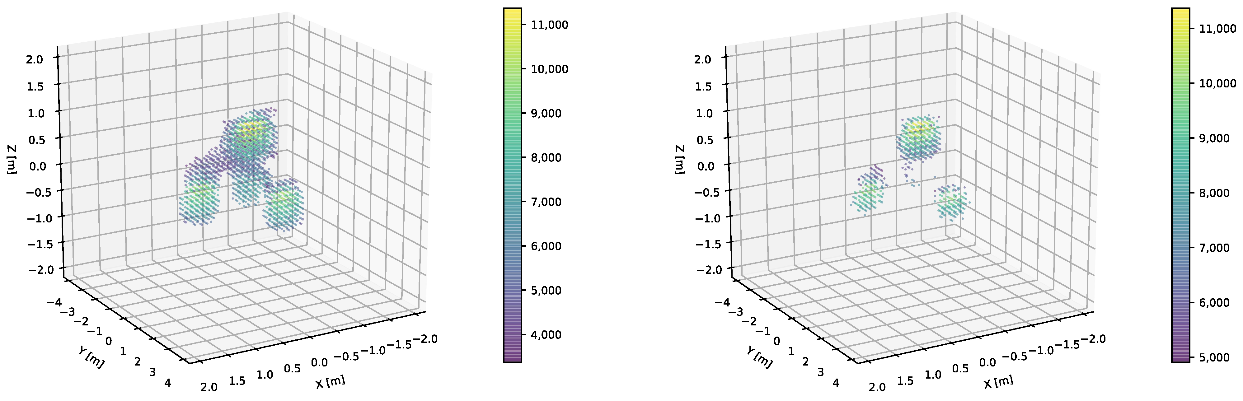
Figure 15.
The 3D voxel map of multiple lead blocks reconstructed with the parameter set optimized for lead as shown in
Table 3 (
left) and the set for multiple lead blocks as shown in
Table 6 (
right). The color of the voxel point represents the combined voxel score
.
Figure 15.
The 3D voxel map of multiple lead blocks reconstructed with the parameter set optimized for lead as shown in
Table 3 (
left) and the set for multiple lead blocks as shown in
Table 6 (
right). The color of the voxel point represents the combined voxel score
.
Table 1.
The nine separate measurements for the different particle types and detector planes.
Table 1.
The nine separate measurements for the different particle types and detector planes.
| | Photons | Neutrons | Electrons |
|---|
| Upper detector | | | – |
| Sidewise detectors | | | – |
| Lower detector—production | | | – |
| Lower detector—absorption | | | |
Table 2.
The position of the four lead blocks.
Table 2.
The position of the four lead blocks.
| | | | |
|---|
| Block 1 | | | |
| Block 2 | | | |
| Block 3 | | | |
| Block 4 | | | |
Table 3.
The parameter set with the noise thresholds optimized for lead.
Table 3.
The parameter set with the noise thresholds optimized for lead.
| | Photons | Neutrons | Electrons |
|---|
| Upper detector | 20% | 10% | – |
| Sidewise detectors | 20% | 10% | – |
| Lower detector—production | – | 10% | – |
| Lower detector—absorption | 40% | 40% | 40% |
Table 4.
The parameter set with the noise thresholds optimized for water.
Table 4.
The parameter set with the noise thresholds optimized for water.
| | Photons | Neutrons | Electrons |
|---|
| Upper detector | 15% | – | – |
| Sidewise detectors | 15% | – | – |
| Lower detector—production | 15% | – | – |
| Lower detector—absorption | 30% | 30% | 30% |
Table 5.
The parameter set with the noise thresholds optimized for a lead block in water basin.
Table 5.
The parameter set with the noise thresholds optimized for a lead block in water basin.
| | Photons | Neutrons | Electrons |
|---|
| Upper detector | 40% | 30% | – |
| Sidewise detectors | 40% | 30% | – |
| Lower detector—production | – | – | – |
| Lower detector—absorption | 60% | 60% | 60% |
Table 6.
The parameter set with the noise thresholds optimized for multiple lead blocks.
Table 6.
The parameter set with the noise thresholds optimized for multiple lead blocks.
| | Photons | Neutrons | Electrons |
|---|
| Upper detector | 30% | 20% | – |
| Sidewise detectors | 30% | 20% | – |
| Lower detector—production | – | 20% | – |
| Lower detector—absorption | 50% | 50% | 50% |


