Power Quality Impact and Its Assessment: A Review and a Survey of Lithuanian Industrial Companies

Abstract

Poor PQ is a partial case of power system impact on society and the environment. Although the significance of good PQ is generally understood, the topic has not yet been sufficiently explored in the scientific literature. Firstly, this paper discusses the role of PQ in sustainable development by distinguishing economic, environmental, and social parts, including the existing PQ impact assessment methods. PQ problems must be studied through such prisms as financial losses of industrial companies, damage to end-use equipment, natural phenomena, interaction with animals, and social issues related to law, people’s well-being, health and safety. Secondly, this paper presents the results of the survey of Lithuanian industrial companies, which focuses on the assessment of industrial equipment immunity to both voltage sags and supply interruptions, as well as a unique methodology based on expert assessment, IEEE Std 1564-2014 and EN 50160:2010 voltage sag tables, matrix theory, a statistical hypothesis test, and convolution-based sample comparison that was developed for this purpose. The survey was carried out during the PQ monitoring campaign in the Lithuanian DSO grid, and is one of the few PQ surveys presented in the scientific literature. After counting the votes and introducing the rating system (with and without weights), the samples are compared both qualitatively and quantitatively in order to determine whether the PQ impact on various end-use equipment is similar or not.

1. Introduction

It is not a secret that poor power quality (PQ), and in particular short-duration RMS voltage variations caused by power grid faults, still remains a big problem for industry [1,2]. Although the paradigm of the main European PQ standard EN 50160:2010 [3] consists only of voltage events, the main North American PQ standard IEEE Std 1159-2019 [4] encompasses current events as well. From a broader perspective, the PQ field is a part of electromagnetic compatibility (EMC), the core part of which consists of two essential requirements—equipment (apparatus and fixed installations) must be designed and manufactured in such a way (1) that the electromagnetic disturbances it generates do not exceed an allowed level and (2) that it has an appropriate immunity and is able to function as intended in an electromagnetic environment. In Lithuania, this is regulated by both the EMC Directive 2014/30/EU [5] and national Technical Regulation [6], and falls under the responsibility of the Communications Regulatory Authority of the Republic of Lithuania. It is understandable that the requirements for the immunity must be stricter than for the emissions. In addition, it is worth mentioning that according to IEEE Std 1159-2019, IEC standards classify causes of electromagnetic disturbances (or, in other words, causes of electromagnetic interference) into conducted low-frequency, conducted high-frequency, radiated low-frequency and radiated high-frequency phenomena as well as into electrostatic discharge phenomena and nuclear electromagnetic pulse. All mentioned aspects are faced in a complex manner: end-user equipment, when working in the electromagnetic environment, must be both resistant to all types of electromagnetic interference and not emit it—this can be represented by the overlapping area of Venn diagrams given in Figure 1. Moreover, the scientific literature is increasingly beginning to examine PQ of DC grids—this new PQ subject is not yet included in both EN 50160:2010 and IEEE Std 1159-2019, but is relevant and needs to be investigated in anticipation of, for example, massive advent of microgrids and Power-to-X systems.

PQ is mostly related with conducted phenomena, but there are also some other cases, such as lightning-induced overvoltages, geomagnetic storm effects, and the coupling between electrocardiogram signal and power wires that is described in the PQ analyzer manufacturer’s webpage [7]. In general, when assessing PQ impact, it is useful to analyze both voltage and current data because, for example, most voltage sags are caused by high current demand, which is also dangerous and not desirable phenomenon [2,8].

The aim of this paper is to study the effects of poor PQ and their assessment methods. In addition to the literature review, this paper presents the survey of Lithuanian industrial companies focusing on the immunity to conducted electromagnetic interference (more precisely, to short-duration RMS voltage variations—voltage sags and supply interruptions).

2. Literature Review

The impact of electric power systems is multifaceted and must be continuously studied from various angles. One of the most well-known negative factors is undoubtedly the burning of fossil fuels—carbon dioxide CO₂, sulfur dioxide SO₂, and nitrogen oxides NO_x along with other gas and particulate matter emissions directly contribute to global warming, poor air quality, acid rains, etc. It is not a secret that although many technologies such as electric vehicles and energy production using renewable energy sources seem to be eco-friendly, they have many side effects. Hydropower can cause drought conditions downstream, affects fish migration, reduces the oxygen level in the water, reservoirs are subject to eutrophication (which is caused by excessive concentration of plant nutrients, primarily phosphates and nitrates) as well as produce carbon dioxide and methane emissions, water release from a reservoir can alter the temperature of the water downstream, etc. Solar and wind parks, not to mention their production process and utilization issues, can not only emit such PQ phenomena as harmonics and flickers, but also reduce the area of grasslands, which are important to birds of prey for hunt and feed (e.g., this factor is mentioned in [9], which describes the opposition from the local residents to the construction of the wind park in Širvintos municipality) and, for instance, as a habitat for roe deer (Capreolus capreolus) fawns. Further, according to [10,11], wind park noise can scare animals away and pose a risk of interference in their communication. Habitat loss is also caused due to vegetation clearing around power lines, which is necessary to avoid contact and accordingly PQ events: on the one hand, [10] cites two negative examples of great bustard (Otis tarda) and bearded vulture (Gypaetus barbatus) and, on the other hand, it cites one positive example of when “vegetation clearing affected positively some endangered bird species […] that use [forest] edges as nesting habitats”.

Another relevant example is the effects of electromagnetic fields. This topic covers not only the fields created by 50 Hz, 60 Hz, 400 Hz and other frequency power systems, but also the higher frequency fields created by Smart Grid communication networks (see [1] for more information): for example, the highest frequency of 5G NR Frequency Range 2 is 71 GHz. Although neither 50 Hz nor 71 GHz radiation is ionizing and these frequencies are lower than the frequencies of the visible spectrum (400–790 THz approximately), this does not mean that there cannot be any biological or health effects, concerns and their studies. Exposure of living organisms to either power frequency or radiofrequency fields induces currents inside their bodies: this can result in heating of body tissues, and the main variables influencing such interaction are the frequency of the field, the intensity of the field, the length of exposure, the polarization of the field, the modulation of the signal, and the dielectric characteristics of the affected tissues [12]. According to the World Health Organization [13], “it is not disputed that electromagnetic fields above certain levels can trigger biological effects”, but since the reference levels of electric, magnetic and electromagnetic fields are regulated by various documents (e.g., Council Recommendation 1999/519/EC [14], IEC 61000-6-3:2020 [15], IEC 61000-6-4:2018 [16]), the main question is whether long-term low-level exposure to such radiation can somehow affect one or another group of humans or animals. Such effects can be thermal and non-thermal [17]. For example, the studies reviewed by [12] revealed that both near-field and far-field exposures within permissible limits can cause headache, fatigue, sleeping disturbances, temperature changes, anxiety, lack of concentration, itching, nausea, etc., and the studies reviewed by [17] found various negative impacts on antioxidant defense system (which controls the formation of free radicals and prevents their harmful effects, including the damage to DNA), resulting in oxidative stress, which is the driving force for cancer and many other diseases. Nonetheless, the World Health Organization [13] notes that no adverse health effects (including carcinogenicity, pregnancy outcome, and cataracts) from such low-level long-term exposure have been confirmed to date. On the other hand, it must be understood that massive use of mobile phones as well as other information and communication technologies is the occurrence of mainly the last decade which is not sufficient for the generalization of such complex studies.

PQ impact is a partial case of energy systems impact. Such studies are important, for example, in anticipation of predictive maintenance [1,8]. Poor PQ, and in particular voltage sags and supply interruptions, can have various consequences: for example, in [8], they are divided into two mutually related parts—damage to equipment and caused outages. Despite the fact that it is generally understood that PQ phenomena are harmful to both end-use equipment and electricity network infrastructure, interrupt technological processes, interfere with maintaining a proper work mode and thus negatively affect the quality of the manufactured products, cause financial losses, and pose a risk to environment, health and safety, there is still not enough information and comprehensive studies on the topic as well as their practical value. Inspired by [18], a brief look at PQ impact from a new angle—through the prism of sustainable development—is presented in Figure 2. It is an approach that tries to find a balance between economic development, environmental protection and social well-being. Detailed examination of these parts is continued in Section 2.1, Section 2.2 and Section 2.3

2.1. Economic Impact

The economic impact of PQ can be direct and indirect: (1) direct cost includes loss of production during continuous operation, loss of resources and time, waste in semi-finished production, restart of process, equipment damage, costs associated with human safety and health, environmental financial penalties, as well as utility costs due to interruptions; (2) indirect cost includes the costs due to production delay and the financial cost of loss of market share [19,20,21]. Each factor depends on the user and its technological process and has a different weight. It also depends on the PQ phenomenon. For example, according to the information reported by [22] (2007), in the case of the annual energy consumption of 1–5 GWh, the total annual loss experienced by the three Slovenian industrial companies due to voltage sags was EUR 180,000 (i.e., on average EUR 60,000 per company) at the prices of either 2007 or earlier year, EUR 800,000 by the eight companies due to short interruptions, EUR 40,000 by the one company due to harmonics, EUR 100,000 by the two companies due to voltage transients, in the case of the annual consumption of 5–25 GWh, EUR 1,380,000 by the four companies due to short interruptions, in the case of the annual consumption exceeding 25 GWh, EUR 760,000 by the five companies due to voltage sags, EUR 950,000 by the eight companies due to short interruptions, etc. According to [23] (2012), the financial losses per voltage sag event suffered by nine United Kingdom industrial consumers at prices of either 2010 or earlier year were GBP 18,300 by the pulp and paper plant, GBP 152,500 by the metalworking plant, GBP 4366 by the food processing plant, GBP 15,250 by the textile plant, GBP 3,344,000 by the semiconductor fabrication plant, GBP 45,750 by the automotive assembly plant, GBP 30,500 by the chemical plant, GBP 61,000 by the equipment manufacturing plant, and GBP 18,300 by the plastic extrusion plant, and it was mentioned that the most sensitive equipment is AC contractors, variable-frequency drives, programmable logic controllers and personal computers. Other information from two sources about the economic impact of voltage sags at the prices of 2001 or earlier year is available in [24] (2022, p. 163): (1) until 2001, typical financial loss per voltage sag event suffered by semiconductor production business was EUR 3,800,000, EUR 6,000,000 per hour by financial trading, EUR 750,000 by computer centers, EUR 30,000 per minute by the telecommunications industry, EUR 350,000 by steelworks, and EUR 250,000 by the glass industry; (2) in the United States until 2001, the financial impact of one voltage sag event in paper manufacturing was USD 30,000, USD 50,000 in the chemical industry, USD 75,000 in the automobile industry, USD 100,000 in equipment manufacturing, USD 250,000 in credit card processing, USD 2,500,000 in the semiconductor industry, and the annual impact was over USD 20 billion. Perhaps it can be guessed that such losses nowadays should be lower due to higher industrial flexibility, a higher level of both grid automation and distributed generation penetration, and various other factors—this topic remains for further research.

Let us compare the equations for estimating the financial impact of voltage sags and harmonics given in [19]. Although they both at first glance seem to be quite simple, their application in practice by evaluating all the technical and economic variables is not an easy task (which is one of the reasons for the lack of scientific literature on this topic). In the case of voltage sags, total financial losses for a consumer can be calculated by the following equation:

$$TL=MV-CM-CE+AC,$$

(1)

where $MV$—market value of products that could have been produced during downtime; $CM$—material cost that could have been used in production process; $CE$—energy cost that could have been used in production process; $AC$—additional costs suffered due to supply interruption. Economical damage caused by harmonics can be calculated as follows:

$$D=D_w+D_a,$$

(2)

where $D_w$—operational costs associated with increased energy loss; $D_a$—ageing costs associated with the heating effects. The operating temperature of both motors supplied by non-sinusoidal waveform and transformers feeding non-linear loads is higher due to the increase in eddy currents [25], and the dissipated power is proportional to their frequency:

$$P={\displaystyle \frac{{\pi }^2}{6kD}}·{\displaystyle \frac{{B_p}^2{f}^2{d}^2}{\rho }},$$

(3)

where $P$—power lost per unit mass, W/kg; $k$—constant equal to 1 for a thin sheet and 2 for a thin wire; $B_p$—peak magnetic field flux density, T; $f$—frequency, Hz; $d$—thickness of the sheet or diameter of the wire, m; $D$—density of the material, kg/m³; $\rho$—resistivity of the material, Ωm [26,27].

Reliable operation of both power grid and end-use equipment is a key factor in avoiding economic losses. For example, incorrect tripping of relay protection can be caused by either voltage sag (due to voltage drop not only in the network but also in the secondary circuits) or harmonics, which puts consumers at risk of experiencing a supply interruption and consequent outage. Also, as is seen from the results of the survey of Lithuanian industrial companies (Section 4), the failure of a single chain/device of a technological line in most cases causes the stoppage of the entire line: restarting an interrupted technological line is a hard and time-consuming task, as it is necessary to remove the remaining damaged products and materials which are no longer suitable for use. Obviously, sequential technological processes are more common and are more vulnerable than parallel. A sequential process stops if at least one of its elements fails, and a parallel process stops only if all of its elements fail. In mathematical terms, the reliability of a sequential process, which is composed of $i$ elements and when all of them are dependent, is:

$$P=\prod _i{(1-P}_i),$$

(4)

while the reliability of a parallel process, when all elements are independent, is:

$$P=1-\prod _i{P}_i,$$

(5)

where $P$—probability of continuous process operation (reliability); $P_i$—failure probability of the process element with index $i$.

Although studies on the impact of PQ on the equipment and its severity assessment algorithms are very important and will have great practical significance (as a part of predictive maintenance and outage management), their execution is full of challenges at least due to the reasons mentioned in [1,2,8]—scientific immaturity of the PQ field, deficiency of PQ monitoring systems, hardly predictable nature of PQ phenomena, laboratories required for both artificial generation of PQ phenomena (voltage sags, impulses, etc.) and immunity testing, etc. The ageing process is natural for all equipment and worsens its characteristics (e.g., degrades the dielectric properties of insulation, LED devices experiences lumen deprecation and chromaticity shift, etc.), and the main goal is to accurately quantify the negative impact of PQ phenomena and their contribution to the acceleration of the ageing processes. Such damage will depend on the type of device, operating conditions, type of PQ phenomenon, its parameters, quantity, exposure time, etc.: for example, in the case of insulation, the task is to evaluate the influence of the number of both voltage transients and swells, their parameters and shape as well as insulation operating conditions (temperature, humidity, mechanical stress, chemical environment, radiation, etc.) on such characteristics as breakdown voltage and loss angle, and in the case of harmonics—the influence of harmonic frequency, sequence, magnitude and exposure duration on vibration of rotating machines, thermal effect and, for instance, its impact on chemical reactions in LED materials.

When testing the immunity to RMS voltage variations, the results should be presented in the voltage–duration plane by drawing a curve that separates zones where equipment operation remains uninterrupted and where it is interrupted with all the consequences that follow. The goal is to draw these curves for each device and, when necessary, for a group of them by evaluating all influencing factors. The severity of voltage sags depends on various factors, such as voltage sag depth, duration, shape, energy, and point on wave. Further, it depends on the device and its operating mode: for example, [28] demonstrates that the immunity of the tested LV three-phase induction motor (746 W) depends on its loading. A case study on residual voltages at the terminals of induction motors after a three-phase short circuit at various grid nodes is presented in [2], and if their immunity curves were known, it would be possible to predict the probability of their work continuity which directly correlates with the reliability of the technological process and financial losses. Next, Figure 3 presents several immunity test results of the LV single-phase equipment found in [24,29,30]: it can be seen that the most sensitive of the examples given is variable-frequency drive, the operation of which is interrupted when the voltage drops below 0.8 p.u. Contrary to other appliances, electric motor recovery after a voltage sag is followed by inrush current that causes another voltage sag which not only interferes with the recovery but also can affect other loads. The presented examples are subject to the limitations of inductive reasoning: these results are case-specific and, at present, the number of such studies is clearly insufficient for generalization.

To continue, the first question that arises is what should be the benchmark for the voltage sag immunity requirements. Naturally, there is a desire for the equipment to be fully resistant, but this is limited by cost and other real-world factors. At the moment, there are several universal reference curves established for end-use equipment, of which the most well-known probably are the SEMI F47, ITIC, and IEC 61000-4-11 (identical to IEC 61000-4-34). It is noteworthy to mention that the opposite of these curves is fault-ride-through requirements for power-generating modules—PQ phenomena are dangerous not only for end-use equipment but also for generators by posing a risk of their disconnection, which negatively affects the reliability of electric power systems as well as hinders electricity trading. Plotting the curve is a qualitative assessment, thus the second question that arises is how to quantify the severity of voltage sags. For this, it is necessary to introduce various indexes that would give the weights to the regions of the voltage–duration plane. For example, [31] does this by creating the feature vector with five—grid energy loss, voltage sag value, voltage sag duration, equipment tolerance (by using the rectangular curve as a reference), and equipment compatibility (by using the SEMI F47 and ITIC curves as a refence)—indexes, and justifiably criticizes other sources that uses only either one or two indexes, because such approach perhaps cannot be completely objective and reasonably reflect the situation. Among these sources is IEEE Std 1564-2014 [32]—this guide for voltage sag indexes provides the methodology for voltage sag severity evaluation by using the SEMI F47 curve as a reference. SEMI F47 is a globally used standard (originally published in 2000, updated in 2006), which defines minimum voltage sag immunity requirements by setting out the limits that the equipment needs to tolerate without creating any process upsets or shutdowns. Equipment is not classified by type, but the primary focus of the specification is semiconductor processing equipment (e.g., etching, film deposition, photolithography equipment, etc.) and the secondary focus is subsystems and components that aid in the semiconductor manufacturing process (e.g., computers, robots, AC relays, variable speed drives, etc.) [33]. The SEMI F47 curve is more stringent compared to the ITIC curve and other curves given in IEEE Std 1564-2014. Standards play a very important role in the PQ field [1], thus, in spite of the criticism, this is one of the currently best-developed and methodologies suitable for both scientific and practical studies: for example, [34] uses it to assess voltage sags in distribution systems with fast charging stations, and [35]—for analyzing measurement data of the 13.2 kV busbar of the Colombian grid. The methodology of IEEE Std 1564-2014 is appropriate for this paper as well—it will be presented in detail in Section 3.2 and, together with other methods, will be used to assess the results of the survey of Lithuanian industrial companies.

Another no less important research area, which also has a lot of gaps, is the immunity to other PQ phenomena. In [36], a focus is made on the impact of DC PQ (ripples, harmonics) on water electrolyzers: it has been found that current ripples generate additional losses in the electrolyzer cell, negatively affect hydrogen production and its energy efficiency, and further works should also concentrate on their impact on the cell degradation. The effects of voltage harmonics on dielectric losses and dissipation factor in HV insulating materials as well as their measurement results fall under the scope of [37]: voltage harmonics due to additionally added fast changing slopes $dU/dt$ shorten insulation lifespan, may result in additional losses and the acceleration of partial discharge development, as well as their presence complicates dielectric loss measurement and can lead to misinterpretation of the results. Voltage harmonic immunity requirements for adjustable speed electrical power drive systems are specified by IEC 61800-3:2022 [38]: the requirements for levels at the LV equipment terminals are set directly, but for the MV equipment—with a reference to IEC 61000-2-4:2024 [39]. A comparison with the requirements of EN 50160:2010 (which are identical for LV and MV networks) is presented in Figure 4. It can be seen that the immunity requirements for the equipment within the scope is stricter than the values of EN 50160:2010, and that IEC 61800-3:2022 sets limit values up to the 40th harmonic, while EN 50160:2010—up to the 25th, but not for all. The requirements for immunity to short-term voltage harmonics (less than 15 s) as well as the requirements for current harmonic values at agreed point of coupling are also given in IEC 61800-3:2022. It must be explained that the compliance with the standard does not mean that harmonics within permissible limits will not have an effect—this is more related to the general assessment of performance to determine whether it is satisfactory or not. Harmonics are classified into even and odd by distinguishing multiples from not multiples of 3, as well as into positive, negative, and zero sequence: positive sequence harmonics (1st, 4th, 7th, 10th, 13th, etc.) rotate in the same direction as the fundamental, negative sequence harmonics (2nd, 5th, 8th, 11th, etc.) rotate in the opposite direction, while zero sequence harmonics (3rd, 6th, 9th, 12th, 15th, etc.) do not rotate. Negative sequence harmonics can weaken the mechanical torque of an electric motor, while zero sequence harmonics can cause overheating of the neutral.

Information about the impact of voltage unbalance on induction motors can be found in [40] (pp. 596–602). Its nature is threefold: (1) unbalanced power supply from the mains; (2) non-symmetric impedance in either stator or rotor; (3) asymmetrical winding configuration (connection). The unbalance is not always disadvantageous and sometimes can be intentionally used to achieve exceptional characteristics of electric machines; however, in the case of the induction motor designed for a symmetrical power supply, voltage unbalance results in the negative sequence torque $M_2$ adding to the positive sequence torque $M_1$, which distorts the torque–slip characteristic $M\left(s\right)$, causes vibrations, reduces motor efficiency, and poses a risk of mechanical breakdown. In the case of an induction machine, the equation of the total electromagnetic torque is obtained by knowing the parameters of two—positive sequence and negative sequence—T-type equivalent circuits:

$$M=M_1+M_2=\left(m_1{I_{21}^{\prime }}^2{\displaystyle \frac{r_{21}^{\prime }}{s}}-m_1{I_{22}^{\prime }}^2{\displaystyle \frac{r_{22}^{\prime }}{2-s}}\right){\displaystyle \frac{p}{{\omega }_1}},$$

(6)

where $m_1$—number of phases; $I_{21}^{\prime }$—secondary current in the positive sequence T-type equivalent circuit; $I_{22}^{\prime }$—secondary current in the negative sequence T-type equivalent circuit; $r_{21}^{\prime }$—secondary resistance in the positive sequence T-type equivalent circuit; $r_{22}^{\prime }$—secondary resistance in the negative sequence T-type equivalent circuit; $s$—slip; $p$—number of pole pairs; ${\omega }_1$—angular frequency of rotating magnetic field produced by the main harmonic.

2.2. Environmental Impact

The interaction between PQ and the environment is twofold: on the one hand, natural factors can cause PQ events, and on the other hand, there is also an anthropogenic component when PQ events affect the environment. The effects range from small voltage sags to power system blackouts and serious ecological consequences. PQ events can disable critical equipment whose operation is essential for human and environmental security. These include fire-fighting pumps, equipment preventing air pollution (such as electrostatic precipitators which remove particles from a flowing gas using the force of an induced electrostatic charge, and flue-gas desulfurization process during which sulfur dioxide is removed from exhaust flue gasses of fossil-fuel power plants as well as petroleum refineries, waste incineration, cement and lime kilns), wastewater treatment facilities, as well as nitrogen loops used for chemical inerting (to reduce and inhibit undesirable chemical reactions with oxygen), and cooling loops in nuclear power plants, nuclear waste repositories, and oil refineries [1,2].

To start with, among the primary causes of PQ events, in particular supply interruptions, are natural hazard events such as windstorm, lightning, earthquake, tsunami, and flood. The example of the Fukushima Daiichi nuclear disaster, which was caused by the 2011 Tōhoku earthquake and tsunami as well as their impact on both the power grid supplying the power plant and the nuclear reactor cooling systems, has already been discussed in [2]. The impact of the extreme weather on the reliability of the United States power system, including the history of blackouts, is discussed in [41]: between 1984 and 2012, as can be seen from the graph given in [42] (p. 3), the annual number of the major outages (i.e., those that affected at least 50,000 customers) caused jointly by the categories labelled “storms and severe weather”, “cold weather and ice storms”, “hurricanes and tropical storms”, “tornadoes” and “extreme heat and wildfires” increased drastically (including because of stricter reporting requirements), and between 2003 and 2012, “80% of all outages were weather related”. In [43], a focus is made on a qualitative assessment of the impact of so-called Winter Storm Uri, a series of winter storms in Texas on 13–17 February 2021, on power system resilience: abnormally cold weather led to widespread disruption in electricity generation (particularly from natural gas) and to a spike in electricity demand (which exceeded the projected winter peak demand of 57.7 GW by over 10 GW), the grid operator enforced load shedding (which prevented the frequency from falling below 59.3 Hz), the state suffered a major power crisis. Analysis of severe scenarios and their consequences is very important in order to properly prepare for them and perhaps even to prevent (avoid) them: conceptually, [41] illustrates this process with the resilience trapezoid by dividing the timeline into the pre-disturbance resilient state, the disturbance progress, the post-disturbance degraded state, the restorative state, and the post-restoration state, while [43] illustrates this with a resilience curve by dividing the timeline into preparation, absorption, recovery, and adaptation phases.

In addition to extreme situations, there are also smaller-scale but no less important events that cause short circuits and worsen grid reliability indexes. Thunderstorms are directly related to the occurrence of voltage spikes and transients, high winds and minor storms cause conductor gallop, increase a risk of tree toppling and their branches falling. However, this topic has not been deeply explored in the literature and remains an open research field [2,8]. In Lithuania, most lightning strikes occur between the end of spring and the beginning of summer and, as can be seen from the map given in [1], the territory of the country is divided into two zones regarding annual thunderstorm duration—up to and more than 40 h. According to [41], weather is responsible for Minnesota Power high SAIFI and SAIDI values: in 2015–2016, as can be seen from the circular diagrams, the share of weather-related events in SAIFI was 72% and in SAIDI was 27%. In Lithuania, as can be seen from the statistical data of 2015–2018 given in [2], which uses a different data classification and aggregation method, most 10 kV grid faults are caused by flora (including both weather-related and non-weather-related events) with an expected rate (mode of a probability density function) above 1200 per year, followed by cable line failures with an expected rate above 700 per year, lightning and lightning arrester failures, fauna, and insulator failures, while the expected number of conductor gallop events per year is approximately equal to 30; however, the influence of these groups on SAIFI and SAIDI values has not been estimated (only the general assessment of the dependence on the total number of events has been performed by means of regression analysis, which does not reveal the whole picture).

Another aspect is the relationship between fauna and short circuits. In [10], twelve abiotic impacts of electric power systems on biodiversity (including plants) are distinguished—the barrier effect, line as a resource, habitat conversion, habitat fragmentation, edge effects, electromagnetic field, the corridor effect, habitat loss, fire risk, the noise effect, air pollution, as well as soil degradation and hydrological alterations. The aspect under consideration falls as a partial case under the scope of the first two topics: (1) the ‘barrier effect’ is a topic that includes animal contact (collisions) with power grid infrastructure, modification of animal behavior in response to the presence of physical obstacles, as well as other factors (e.g., [10] mentions that power line corridors, especially when combined with roads, affects the distribution and density of ungulates which can be caused by a higher risk of predation, poor foraging conditions, hindered movement and decreased habitat quality, for small arboreal mammals—this results in the loss of canopy connectivity, and for salamanders—this potentially limits the population connectivity); (2) ‘line as a resource’ is a topic about bird species that use power grid structures for nesting and as a foraging perch: on the one hand, this is beneficial for both individuals and their populations, while on the other, this poses a risk of bird electrocution. A collision must be distinguished from an electrocution—a contact with conductors can either cause a short circuit or not: (1) if an animal touches one wire, the cause of death or injury will be mechanical but not electrical and therefore it will not result in a short circuit (except for the case if a sufficient potential difference is formed between bird’s feet, which probably remains a hypothetical scenario), but (2) if an animal touches two points of different electric potential (i.e., either two phases or phase and ground), it will result in both its death/injury and a short circuit.

However, at the moment is difficult and therefore studies do not orient towards finding out the proportion between collisions, electrocutions, caused PQ events, their parameters and influence on grid reliability indexes [2] by categorizing the data according to species, grid voltage, transmission tower structure and other relevant criteria. Most studies focus only on the calculation of victims in a certain period of time: for instance, according to the results of [44], in 2011, 161 birds were found beneath the power lines under investigation in the Indian state of Rajasthan between 31 November and 6 December, including 59 house crows (Corvus splendens), 47 Indian rollers (Coracias benghalensis) and 18 Eurasian collared doves (Streptopelia decaocto), and according to the results of [45], in September 2007, more than 70 bird carcasses were found under the inspected power grid section in the Mongolian steppe (data are segregated into birds found under the poles by their type and birds found under the lines), including common kestrels (Falco tinnunculus), golden eagles (Aquila chrysaetos), little owls (Athene noctua), Pallas’s sandgrouses (Syrrhaptes paradoxus), saker falcons (Falco cherrug), steppe eagles (Aquila nipalensis), and upland buzzards (Buteo hemilasius). Nonetheless, several examples can be found when the number of birds found under power lines is divided into collisions and electrocutions. For instance, during the study presented in [46], a total of 4353 victims was found beneath the power lines under investigation in Slovakia between December 2014 and February 2016: the largest number of victims were common buzzards (Buteo buteo)—1028 (3 by collision, 1025 by electrocution), followed by 606 (5 by collision, 601 by electrocution) common magpies (Pica pica), 218 (6 by collision, 212 by electrocution) hooded crows (Corvus cornix), 189 (all by collision) mute swans (Cygnus olor), etc. During the study presented in [47], a total of 43 victims was found beneath the power lines under investigation in the Putalibazar Municipality of the Syangja district of Nepal from November 2021 to May 2022, including 13 (2 by collision, 11 by electrocution) house crows (Corvus splendens), 7 (6 by collision, 1 by electrocution) Indian mynas (Acridotheres tristis), and 6 (1 by collision, 5 by electrocution) rock doves (Columbia livia). However, it should be noted that in these studies, the cause of death was decided by examining the carcass of the killed birds, and not by analyzing PQ measurement data.

According to [48] (p. 14), bird electrocution is a worldwide problem identified especially on the MV power lines (1–52 kV) and railway infrastructure—it is probably reasonable to believe that a transmission grid is safer than a distribution grid in terms of bird electrocutions due to the greater distances between the wires. Examples of animal interactions with electricity grid depend on geographic location and include not only birds: for instance, the collisions of a bald eagle (Haliaeetus leucocephalus) with power lines in the United States are described in [49,50], a leopard (Panthera pardus) that was electrocuted after climbing up an electric pole in India in [51], the electrocution of an Asian elephant (Elephas maximus) by a sagging power line in [52], by a fallen power line (which purportedly was pushed by the animal) in [53], and the electrocution of an Indian python (Python molurus) by a 11 kV line (resulting in the supply interruption for more than 600 houses) in [54]. Electrocution can be the main factor of population decline (e.g., see [55], which studies the endangered populations of Bonelli’s eagle (Aquila fasciata) in Southern Europe, particularly in the Iberian Peninsula); however, the overall effect of electrocution on population dynamics is still unknown for most species [10,48].

As can be seen from the statistical data of the Lithuanian 10 kV grid provided by [2], in 2015–2018, fauna caused 980 faults in the overhead power lines, 852 faults in the outdoor and modular substations (approximately 30% by birds, approximately 50% by rodents), and 336 faults in the pole mounted substations (approximately 80% by birds). According to the results presented in the “LIFE Birds on Electrogrid” final report [56], 254 birds were found beneath the investigated power lines of the Lithuanian TSO (Litgrid AB) during the project period between June 2014 and December 2018, including 112 mute swans (Cygnus olor)—852 km were monitored walking on foot. Concrete conservation actions were: (1) installation of bird collision mitigation measures in bird staging areas (see [56,57] for more details); (2) installation of line markers in the most critical areas (see [56,58] for more details); (3) installation of bird protection measures—“wishbone” type (prevents birds from making a touchdown on the insulators) and “saucer” type (prevents bird excrements from falling on the insulators) installations—on the utility poles, aiming to reduce the mortality rate of the white stork (Ciconia ciconia) due to electrocution (see [56,59] for more details); (4) improvement of breeding conditions of the common kestrel (Falco tinnunculus) by erecting nest boxes on the pylons of the HV lines (see [56,60] for more details). The interim activity report [61] underlines the effectiveness of the measures by comparing the situation in 2014 (ex ante) with 2015 (ex post): (1) it is not always possible to find bird remains; therefore, cases where the cause of disconnection is not determined are relevant as well, because it is probable that they occurred due to bird impact; (2) in 2014, 79 disconnections were recorded due to bird impact or undetermined causes, and most of them occurred during stork migration (automatic circuit reclosing was triggered in almost all cases and was mostly successful); (3) in 2015, only 2 disconnections due to bird impact were recorded in sections where the mitigation measures were installed. The final report [56] concluded that only 12 cases of disconnection of the HV lines were registered in 2017, in comparison to 79 disconnections before the project started. According to experts, in Lithuania, the annual toll of up to 45 thousand bird deaths caused by collisions with the HV lines occurs: the annual toll of 11.1 deaths per 1 km occurs when visibility increasing measures are not installed, and the annual toll of 3.6 deaths per 1 km—when visibility increasing measures are installed [2,56].

To continue, a comprehensive overview of up-to-date knowledge of electrocutions and collisions of birds across 27 European Union member states is presented in [48]: the Slovak report provides information about the relevant characteristics of the electricity networks, bird electrocution mechanism, most vulnerable species, mitigation measures and their effectiveness, as well as legislation and policy framework. After interviewing the national experts, the collected data about most frequent bird victims are summarized in

Table 1. Most frequent victims of power grid in the European Union (as reported by countries) [48].

Species 1,2,3	AT	BE	BG	HR	CY	CZ	DK	EE	FI	FR	DE	GR	HU	IE	IT	LV	LT	LU	MT	NL	PL	PT	RO	SK	SI	ES	SE
A. adalberti																										e
A. albifrons																	○ 4						c
A. anser							c										○ 4			c
A. chrysaetos																	e 5										e
A. cinerea													c				○ 6							c			c
A. fasciata																										e
A. gentilis																	○ 5										e
A. platyrhynchos						c					c						c 7			c				c
B. bubo	e								e	e		e					○ 8								e		e
B. buteo			c/e	e		e				e	e		e		e		e 5				e	e	e	e	e
B. ibis																						c
C. ciconia	e	e	c/e	e	e					c/e	e	e	e				e 9				c/e	e	c/e	e	e	e	c
C. corax			c	e													○10
C. cornix																	○10							e
C. corone											e	e			e							e
C. coturnix					c												○11
C. cygnus							c		c								○12
C. livia		c				c											○13					c
C. olor	c					c	c	c	c			c					c 12			c			c	c			c
C. palumbus		c															○13					c
C. ridibundus		c									c						○14			c
C. undulata																										c
E. alba																	○ 6							c
F. atra											c						○15			c
F. eleonorae					e
F. tinnunculus				e		e				e			e		e		○16	e						e
G. grus													c				○17										c
L. muta															c
L. tetrix															c		○11
M. migrans															e		○ 5
M. milvus															e		○ 5	e
O. tarda	c												c													c
P. apricaria																	c 18
P. crispus												c											c
P. haliaetus															e		○19
P. pica			e			e											○10				e		e	e
P. roseus										c		c
S. aluco				e													○ 8										e
S. uralensis									e								○ 8										e
T. merula						c											○20
T. philomelos					c												○20
T. tetrax																										c

¹ Legend: c—collision, e—electrocution, ○—not marked as a frequent victim, but annually observed species in Lithuania, based on information provided by [63]. ² Full names of the listed bird species: Spanish imperial eagle (Aquila adalberti), greater white-fronted goose (Anser albifrons), graylag goose (Anser anser), golden eagle (Aquila chrysaetos), grey heron (Ardea cinerea), Bonelli’s eagle (Aquila fasciata), Eurasian goshawk (Astur gentilis), wild duck (Anas platyrhynchos), Eurasian eagle-owl (Bubo bubo), common buzzard (Buteo buteo), cattle egret (Bubulcus ibis), white stork (Ciconia ciconia), common raven (Corvus corax), hooded crow (Corvus cornix), carrion crow (Corvus corone), common quail (Coturnix coturnix), whooper swan (Cygnus cygnus), common pigeon (Columba livia), mute swan (Cygnus olor), common wood pigeon (Columba palumbus), black-headed gull (Chroicocephalus ridibundus), African houbara (Chlamydotis undulata), great egret (Egretta alba), Eurasian coot (Fulica atra), Eleonora’s falcon (Falco eleonorae), common kestrel (Falco tinnunculus), common crane (Grus grus), rock ptarmigan (Lagopus muta), black grouse (Lyrurus tetrix), black kite (Milvus migrans), red kite (Milvus milvus), great bustard (Otis tarda), European golden plover (Pluvialis apricaria), Dalmatian pelican (Pelecanus crispus), osprey (Pandion haliaetus), common magpie (Pica pica), greater flamingo (Phoenicopterus roseus), tawny owl (Strix aluco), Ural owl (Strix uralensis), common blackbird (Turdus merula), song thrush (Turdus philomelos), little bustard (Tetrax tetrax). ³ Country names are indicated with ISO 3166-1 alpha-2 codes: AT—Austria, BE—Belgium, BG—Bulgaria, HR—Croatia, CY—Cyprus, CZ—Czech Republic, DK—Denmark, EE—Estonia, FI—Finland, FR—France, DE—Germany, GR—Greece, HU—Hungary, IE—Ireland, IT—Italy, LV—Latvia, LT—Lithuania, LU—Luxembourg, MT—Malta, NL—Netherlands, PL—Poland, PT—Portugal, RO—Romania, SK—Slovakia, SI—Slovenia, ES—Spain, SE—Sweden. There are no data from Latvia, Malta, and Ireland. ⁴ Further, the following species of the genus Anser are also regularly observed in Lithuania: pink-footed goose (Anser brachyrhynchus), taiga bean goose (Anser fabalis), lesser white-fronted goose (Anser erythropus), tundra bean goose (Anser serrirostris). ⁵ Further, the following species of the family Accipitridae are also regularly observed in Lithuania: Eurasian sparrowhawk (Accipiter nisus), rough-legged buzzard (Buteo lagopus), short-toed snake eagle (Circaetus gallicus), western marsh harrier (Circus aeruginosus), hen harrier (Circus cyaneus), pallid harrier (Circus macrourus), Montagu’s harrier (Circus pygargus), lesser spotted eagle (Clanga pomarina), white-tailed eagle (Haliaeetus albicilla), European honey buzzard (Pernis apivorus). ⁶ Further, the following species of the family Ardeidae are also regularly observed in Lithuania: Eurasian bittern (Botaurus stellaris), little bittern (Ixobrychus minutus). ⁷ Further, the following species of the genus Anas are also regularly observed in Lithuania: pintail (Anas acuta), Eurasian teal (Anas crecca). ⁸ Further, the following species of the family Strigidae are also regularly observed in Lithuania: boreal owl (Aegolius funereus), short-eared owl (Asio flammeus), long-eared owl (Asio otus), Eurasian pygmy owl (Glaucidium passerinum). ⁹ Further, the black stork (Ciconia nigra) within the genus Ciconia is also regularly observed in Lithuania: unlike the white stork, it keeps away from people and prefers to construct nests in the depths of the forest (over homesteads and electricity poles). ¹⁰ Further, the following species of the family Corvidae are also regularly observed in Lithuania: western jackdaw (Coloeus monedula), rook (Corvus frugilegus), Eurasian jay (Garrulus glandarius), northern nutcracker (Nucifraga caryocatactes). ¹¹ Further, the following species of the family Phasianidae are also regularly observed in Lithuania: hazel grouse (Tetrastes bonasia), western capercaillie (Tetrao urogallus), grey partridge (Perdix perdix), common pheasant (Phasianus colchicus). ¹² Further, the tundra swan (Cygnus columbianus) within the genus Cygnus is also regularly observed in Lithuania. ¹³ Further, the following species of the family Columbidae are also regularly observed in Lithuania: stock dove (Columba oenas), Eurasian collared dove (Streptopelia decaocto), European turtle dove (Streptopelia turtur). ¹⁴ The only species within the genus Chroicocephalus regularly observed in Lithuania. It was previously placed in the genus Larus. ¹⁵ Further, the following species of the family Rallidae are also regularly observed in Lithuania: corn crake (Crex crex), common moorhen (Gallinula chloropus), spotted crake (Porzana porzana), water rail (Rallus aquaticus), little crake (Zapornia parva). ¹⁶ Further, the following species of the genus Falco are also regularly observed in Lithuania: merlin (Falco columbarius), peregrine falcon (Falco peregrinus), Eurasian hobby (Falco subbuteo), red-footed falcon (Falco vespertinus). ¹⁷ The only species of the family Gruidae regularly observed in Lithuania. ¹⁸ Further, the following species of the family Charadriidae are also regularly observed in Lithuania: little ringed plover (Charadrius dubius), common ringed plover (Charadrius hiaticula), grey plover (Pluvialis squatarola), northern lapwing (Vanellus vanellus). ¹⁹ Classified in its own taxonomic genus Pandion within its own family Pandionidae. ²⁰ Further, the following species of the genus Turdus are also regularly observed in Lithuania: redwing (Turdus iliacus), fieldfare (Turdus pilaris), ring ouzel (Turdus torquatus), mistle thrush (Turdus viscivorus).

—the risk of collision depends on weather, visibility, and location of the power lines sections (whether they cross important bird habitats/breeding areas, main migration routes, etc.), whereas the risk of electrocution depends primarily on technical construction of power facilities. In addition to the already mentioned mute swan and white stork, the wild duck (Anas platyrhynchos), common buzzard (Buteo buteo) and European golden plover (Pluvialis apricaria) are also marked in the Lithuanian column, whereas the already mentioned common kestrel is not. Summing up the total result, most votes were for the white stork: in Lithuania, together with some other countries like Belarus, Latvia, Poland, Ukraine, and Spain (e.g., see [62]), many (more than half) of them nest on power poles during their breeding season (Figure 5a), and then, with the onset of autumn, migrate to Africa as well as some regions of both the Arabian Peninsula and the Indian subcontinent to spend the winter. All bird species breeding and (or) found annually in Lithuania are listed in, for example, [63].

Moreover, there is also the reverse effect, when animals are not responsible for PQ events but nevertheless are killed. In addition, carcasses of killed animals attract the others, which obviously can and will touch a fallen wire as well [64,65,66]: for example, [64] describes the electrocution of both a fox and a bear by a fallen power transmission line in the Russian taiga [65], describes the electrocution of six animals (a rhino, a giraffe, two lions, and two hyenas) in South Africa after storms toppled a power cable, and [66], which is based on the video material of [67], describes the electrocution of foxes (Figure 5b) and other mammals by a fallen power line due to Russo-Ukrainian War. As mentioned in [1,2,8], in Lithuania, such electrocution is possible even under more ordinary conditions: a single-phase fault of an overhead power line of the MV grid can last several hours (until the fault node is physically detected by the electrician brigade, because the resulting voltage unbalance do not propagate through the power transformers [2]), and the contact with such a fallen wire is fatal not only for humans but also for local fauna (Figure 5).

One more aspect to discuss is wildfires. Power grid faults can generate sparks and thus initiate wildfires [68,69,70,71], and even though these faults are not the main cause, this does not devaluate its significance. According to [68], in the Australian State of Victoria, “powerlines cause only 2–3% of all rural fires” under normal conditions, but under extreme fire risk conditions, “this contribution increases dramatically to up to 40–50%”. According to [69], in 2011–2015, electrical power or utility lines caused 14% of all wildfires in the United States, and in 2017–2022, electrical power caused 9% of all wildfires in California (which cannot be directly compared to the aforementioned 14% due to different evaluation practices) but their financial impact was equal to 67%. Probability of ignition depends on such factors as arc duration, wind speed, fuel type (organic matter), and fuel moisture content [72]. Potential causes of fire, not to mention lightning strikes, include many primary causes of PQ events examined in [2], which first cause RMS variations and then other related phenomena—voltage transients and voltage unbalance. From our point of view, these causes can be divided into two groups:

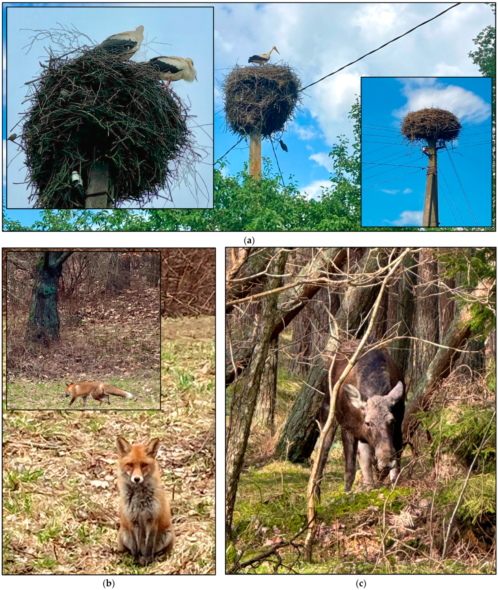
• Vegetation-related faults. These faults are caused by the interaction of wires with trees and bushes. It is not a secret that among the measures to reduce the impact of vegetation are condition monitoring and surveillance of electricity grid infrastructure, vegetation clearing, as well as replacing overhead power lines with underground cables. In Lithuania, according to the statistical data of 2015–2018 provided by [2], the expected annual rate of interaction between the 10 kV grid and a tree outside the safety zone is 845, the interaction with a tree inside the safety zone—95, shrub grow-in events—117, and tree branch drop events—160. In Lithuania, according to the Law of the Republic of Lithuania on Special Conditions of Land Use [73], the safety zone of overhead power lines of up to 1 kV is 2 m in both directions, 6 kV and 10 kV—10 m, 35 kV—15 m, 110 kV—20 m, 330 kV and 400 kV—30 m, and formerly used 750 kV (between the Ignalina Nuclear Power Plant and Belarus)—40 m. Further, it is noteworthy that the safety zone of aerial power cables is 2 m in both directions, underground power cables—1 m, and submarine power cables—100 m. The formation of the safety zones results in a corridor effect—these zones, for example, can facilitate the access of both predators and hunter to ungulates, as well as hinder the movement of some ungulate species, such as the white-tailed deer (Odocoileus virginianus), when there is snow accumulation [10,74,75,76] (in addition to the already mentioned the roe deer and the European moose (Figure 5c), the following ungulate species also live in Lithuania, many of whose main enemies are grey wolves (Canis lupus) and northern lynxes (L. lynx lynx): the wild boar (Sus scrofa), the European fallow deer (Cervus dama), the red deer (Cervus elaphus), the European bison (Bison bonasus), as well as non-native and less common the northern spotted deer (Cervus nippon) (which can mate with native red deer, resulting in the hybrid offspring and thus affecting their own gene pool), the Père David’s deer (Elaphurus davidianus), and the European mouflon (Ovis ammon musimon) [77]).
• Electrical network equipment and infrastructure failures. These are electrical apparatus failures, pole and crossarm failures, and line failures [71]. The first group includes explosions of transformers, circuit breakers, and other oil-filled equipment. The most common type of insulating oil is mineral oil, which, like many other products of crude petroleum, is flammable, explosive and not environmentally friendly. The second group includes such incidents as wooden pole burning due to short circuit, and insulator contamination. In Lithuania, in contrast to, for example, Latvia, wooden poles are not used. Contamination on the surface of the insulators directly and indirectly enhances the chances of flashover by forming a conductive layer on insulator surface, accelerating the corrosion process, causing cracks, etc., and many effects can be prevented through washing: in addition to natural overgrowth with plants, lichens and algae, insulator contamination may be caused by many other factors and materials, such as salt, bird excreta and feathers, weather and its variations, cement, coal, soil, metallic particles, fertilizers, various chemicals, volcanic ash, sandstorms, smog, and smoke (e.g., see [78,79,80,81] for more information). The third group includes sparking during earthed—three-phase-to-ground, two-phase-to-ground, and single-phase—faults, when the wires fall to the ground. In the Lithuanian MV grids, after a single-phase fault, high grounding (capacitive) currents are limited with arc suppression reactors (by creating the conditions for current resonance). According to [82], it is “generally assumed that arcs extinguish by themselves when the arc current is below 5–10 A”. It is worth mentioning that under the appropriate conditions, the extinguished arc can reignite.

2.3. Social Impact

From our point of view, the social impact of PQ can be explained through the prism of both responsibility and liability. It consists of at least three components: (1) responsibility for network pollution with conducted electromagnetic interference, as well as responsibility for ineffective mitigation of it; (2) responsibility dependence on PQ assessment methodology; (3) responsibility for malfunctioning or misfunctioning equipment. At the moment, attribution of legal liability for problems caused by PQ is not widely applied practice due to unfulfilled prerequisites, but individual cases sometimes take place. First, in the field of PQ, attribution of liability is not possible without a fully functioning PQ monitoring system and data analysis skills. Since it is not feasible or cost-effective to monitor every busbar in the grid, research on the propagation of PQ phenomena (including its partial case—identification of the pollution source side) plays a very important role by enabling the prediction of PQ propagation paths [1,2]. In addition to the already mentioned wind and solar parks, there are many other PQ polluters, including variable-speed drives, electric arc furnaces, welding equipment, both AC and DC electrified railways, etc., and each network or device can potentially become a PQ polluter at least due to the unavoidable risk of short circuits. Next, attribution of liability requires fair and transparent legal framework. PQ legislation is mainly composed of standards and, in general, their application is not mandatory (i.e., is voluntary) unless they are mentioned in either national or international legal documents [1]. Harmonized standards have a slightly higher importance: this specific category of European standards can be used to demonstrate that products, services, or processes comply with mandatory technical requirements given in European Union legislation, but their application is also usually voluntary, thus another way can also be chosen to achieve the goal.

To begin with, currently, it is not always possible to apply the PQ legislation due to undetermined limit values. In addition, regardless of the juridical side, the engineering question also arises of when (what) situation is good (acceptable) and when is not. Usually, it is possible to identify the fact of pollution due to a clear PQ definition, but this does not mean a complete quantitative assessment. A considerable amount of research and discussions is still needed in order to sensibly determine permissible limits for the quantity of PQ events and other necessary norms. A brief summary of the current situation is provided below:

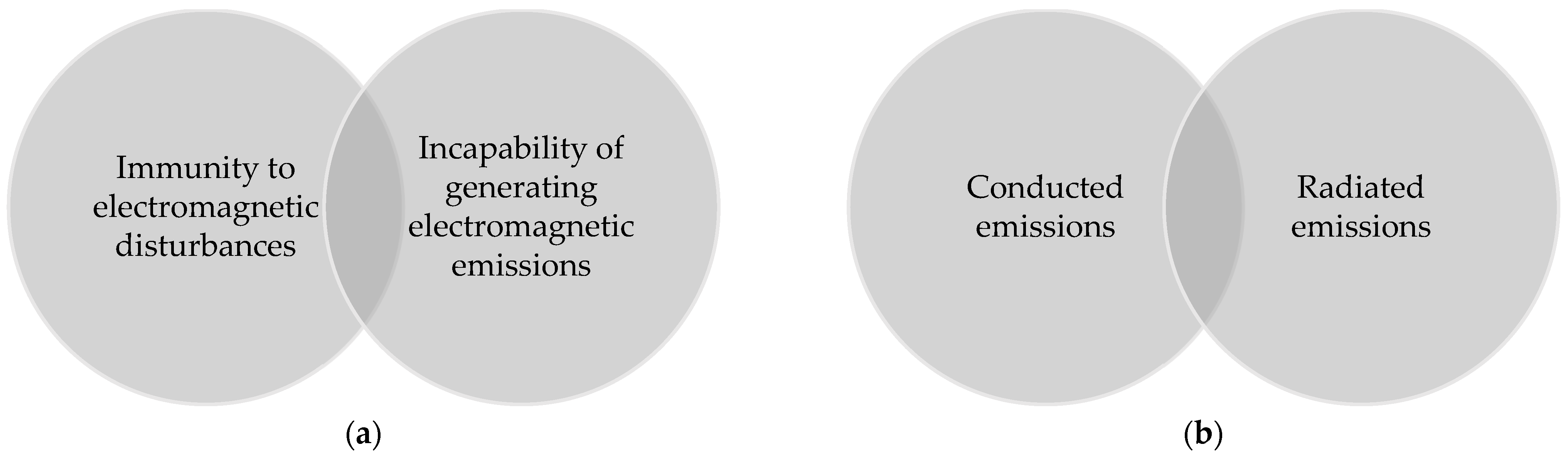
• EN 50160:2010 sets requirements for supply voltage and frequency in normal operation mode, flicker severity, voltage harmonics (up to the 25th, but some levels are still under consideration), voltage unbalance (only negative sequence magnitude), and mains signaling voltage (up to 100 kHz) in public electricity networks with nominal voltages up to and including 150 kV. Limits for rapid voltage changes, voltage sags, voltage swells, supply interruptions, voltage transients, and inter-harmonics are not set. The standard has many gaps which hinder the development of both artificial intelligence (AI) algorithms for PQ assessment and legal acts—some of them are already discussed in [8]. In Lithuania, as in most European countries, this standard is mentioned in the national legal acts and thus is mandatory. In accordance with the Rules for the Supply and Use of Electricity of the Republic of Lithuania [83], the operator, failing to ensure PQ in accordance with EN 50160:2010, must compensate the consumer for the damage caused, excluding the cases of natural phenomena (flood, thunderstorm, frost, sleet, storm, squall, hail, etc.), fire, war, terrorist attack, force majeure, state action, third party action, activation of accident prevention automation, circumstances of necessary action, and many other cases related to the actions or inactions of the electricity consumers.
• IEEE Std 1159-2019 and other IEEE PQ standards do not regulate PQ phenomena, except for IEEE Std 519-2022 [84] which sets limits for both voltage and current harmonics at a point of common coupling. Despite this, IEEE Std 1159-2019 is more informative than EN 50160:2010.
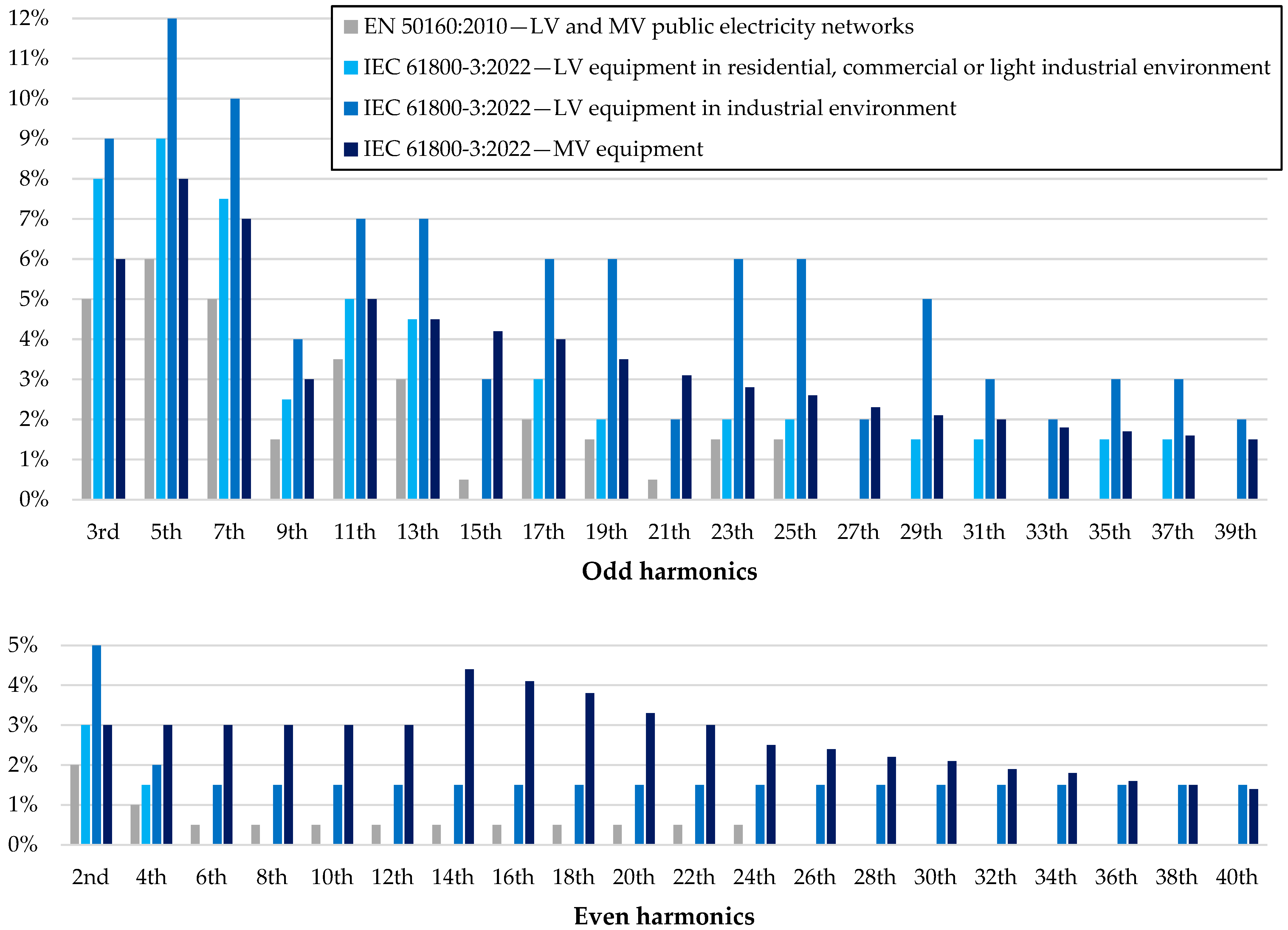
• The harmonized standards under the EMC Directive 2014/30/EU contribute to PQ regulation. IEC 61000-2-2:2002 [85] specifies PQ requirements for public LV electricity networks and supplements EN 50160:2010 by expanding the requirements for voltage harmonic levels up to the 50th, by introducing some requirements for inter-harmonics in the beat frequency range of 0.2–40 Hz (with the fundamental) based on a short-term flicker level of 1 for lamps operated at 120 V and 230 V, as well as by setting the requirements for ripple control system signals in the range of 110–3000 Hz. IEC 61000-2-4:2024 sets PQ requirements for industrial locations with a nominal voltage up to 35 kV, IEC 61800-3:2022—for current harmonic levels in networks with adjustable speed drives depending on the short-circuit power ratio at an agreed point of coupling (common or in-plant). IEC 61000-4-7:2002 [86], IEC 61000-4-15:2011 [87] and IEC 61000-4-30:2015 [88] define the methods for measurement and interpretation of PQ results and therefore play a central role in both EN 50160:2010 and IEEE PQ standards. In Lithuania, as in other European Union countries, EMC standards together with their normative references as well as IEC 61800-3:2022 are mandatory according to the principle of imperativeness of harmonized standards to ensure the compliance with the already mentioned EMC Directive 2014/30/EU.

Probably the most famous example of PQ events is the voltage sag regulation in Sweden, at least just because it has been presented in the 5th CEER Benchmarking Report [89] (2011). It is based on the so-called responsibility-sharing curve which divides the voltage–duration plane into three areas (

Table 2. Classification of voltage sags in Sweden [89,90].

Voltage, p.u.	Duration, s
	0 ≤ t ≤ 0.1	0.1 < t ≤ 0.15	0.15 < t ≤ 0.2	0.2 < t ≤ 0.5	0.5 < t ≤ 0.6	0.6 < t ≤ 1	1 < t ≤ 5	5 < t ≤ 60
Networks above 45 kV
0.9 > U ≥ 0.8	A	A	B	B	B	B	B	B
0.8 > U ≥ 0.7	A	A	B	B	B	C	C	C
0.7 > U ≥ 0.4	A	B	B	B	B	C	C	C
0.4 > U ≥ 0.05	A	B	B	B	B	C	C	C
U < 0.05	A	B	B	B	B	C	C	C
Networks up to and including 45 kV
0.9 > U ≥ 0.8	A	A	A	A	B	B	B	B
0.8 > U ≥ 0.7	A	A	A	A	B	B	B	B
0.7 > U ≥ 0.4	A	A	A	B	B	B	B	C
0.4 > U ≥ 0.05	B	B	B	B	B	B	C	C
U < 0.05	B	B	B	B	B	B	C	C

): (1) voltage sags in Area A are considered as a normal part of operation, expecting that the equipment and installations are sufficiently resistant; (2) the network operator has responsibility to mitigate voltage sags in Area B as much as possible to achieve with state-of-the-art technology at reasonable cost, but no specific limit has been set for their quantity; (3) there shall not be any voltage sags in Area C. Additional information about PQ regulation in Sweden is given by [90] (2011)—the paper presents the division of the voltage–duration plane into three zones for voltage swell assessment in up to 1 kV networks, as well as requirements for the number of rapid voltage changes (taking into consideration both $\Delta U_{\mathrm{s}\mathrm{s}}$ and $\Delta U_{\mathrm{m}\mathrm{a}\mathrm{x}}$ parameters) and duration of supply interruptions. The second example available in [91] (2023) is from the Netherlands. In this case, the voltage–duration plane is divided into four areas (

Table 3. Classification of voltage sags in the Netherlands [91].

Voltage, p.u.	Duration, s
	0.01 ≤ t ≤ 0.2	0.2 < t ≤ 0.5	0.5 < t ≤ 1	1 < t ≤ 5
0.9 > U ≥ 0.8	A	A	A	A
0.8 > U ≥ 0.7	A	A	C	C
0.7 > U ≥ 0.4	A	B2	C	C
0.4 > U ≥ 0.05	B1	B2	C	C
U < 0.05	B1	B2	C	C

) by setting a maximum number of voltage sags allowed based on a 5-year average: (1) sags in Area A are non-severe; (2) the limit in Area B1 for the MV grid is 3, and for the HV and EHV—1.2; (3) the limit in Area B2 for the MV grid is 4, and for the HV and EHV—1.2; (4) the limit in Area C for the MV grid is 4, and for the HV and EHV—0.4. When the limit is exceeded, the network operator shall carry out the investigation and find out the reasons. After the examining the examples provided, it is not difficult to understand that in order to define boundaries between a good, bad, and acceptable situation, a considerable amount of statistical data (monthly, annual) on the actual occurrence of voltage sags is required. Work towards this has already begun. For instance, the available statistical data of 2015–2018 are presented in the 7th CEER Benchmarking Report [92] (2022, pp. 275–282): the situation in the networks of Austria, Belgium, Hungary, Ireland, Kosovo, Portugal, and Slovenia has been assessed by expressing the data as the number of voltage sags per number of monitored points in the voltage sag table of EN 50160:2010 (which will be used in this paper as well); however, for example, the strategies of for selecting monitoring sites are not described, thus it is unclear when a voltage sag caused by the same event was recorder multiple times (i.e., by multiple monitors), and when only once, as well as it is unclear whether PQ mitigation devices was used and what is their impact on the statistics.

Next, by comparing Table 2 and Table 3, it can be noticed that the absence or presence of responsibility (including its severity) is dependent not only on voltage sag parameters but also on their treatment and the structure of the table. Generally speaking, this is dependent on PQ assessment methodology—different methods, formulas, definitions, various uncertainties and gaps can lead to different outcome, data errors and misinterpretation, as well as are an obstacle in the algorithm development process. Let us continue with RMS voltage variations based on the information given by [2] that performs short circuit simulation on the created BRELL-based test grid. EN 50160:2010 requires to take into consideration only one—phase-to-phase for three-wire systems and phase-to-ground for four-wire systems—voltage. Obviously, this is not relevant for three-phase faults since, according to the axiom established by [2], both depths of a symmetrical voltage sag are equal and independent of neutral mode. A few examples are given in Figure 6, Figure 7 and Figure 8: currently, it is not clear (agreed) which assessment method of both two-phase-to-ground and two-phase faults incurs lighter/heavier liability, but it is clear that if only phase-to-phase voltage of the Lithuanian MV and LV grids is considered, in most cases single-phase faults will remain unnoticed (this does not apply to the HV grid). It is noteworthy that, in 2025, after the disconnection of the Baltic power grids from the BRELL system on 8 February and synchronization with the Continental European system on 9 February after the isolated operation test, the obtained results remain completely realistic and valid for Lithuania as well as Latvia, Estonia, Russia and Belarus. The results are valid for other countries’ systems as well, but not necessarily completely due to different features of their networks.

Next example to discuss is the calculation of voltage unbalance. In a three-phase system, negative and zero sequence unbalances are defined as follows:

$$u^{-}[\mathrm{\%}]={\displaystyle \frac{\left|U^{-}\right|}{\left|U^{+}\right|}}·100,$$

(7)

$$u^0[\mathrm{\%}]={\displaystyle \frac{\left|U^0\right|}{\left|U^{+}\right|}}·100,$$

(8)

where $\left|U^{+}\right|$, $\left|U^{-}\right|$ and $\left|U^0\right|$ are magnitudes of the positive, negative and zero sequence phasors, respectively. These magnitudes must be calculated by taking into account the phase angles (i.e., by performing operations with complex numbers). IEC 61000-4-30:2015 notes that algorithms that use RMS values fail to evaluate contributions of angular displacement to these magnitudes, and requires that the voltage unbalance measurement uncertainty of both class A and class B shall not exceed ±0.15%. On the other hand, since symmetrical components are an intermediate result and do not necessarily have to be presented, IEEE Std 1159-2019 (pp. 25–27) provides alternative methods that can be applied by using only RMS measurements without the angle when symmetrical component calculation functionality is unavailable. These alternatives are valid only if phase-to-phase measurements are used, harmonic content is low (in this case, there is no difference between the standard RMS and true-RMS methods—see [8] for more details), and the zero sequence component is zero (as it is in practice when the unbalance is caused by loads, not by earthed faults). The first method is based on ANSI C84.1-2016 [93], which defines voltage unbalance as the ratio of the maximum deviation of a phase-to-phase voltage from the average phase-to-phase voltage to the average phase-to-phase voltage. Mathematically, this can be written as follows:

$$u^{-}[\%]={\displaystyle \frac{\max \left\{\left|\left|U_{\mathrm{m}\mathrm{a}\mathrm{x}}\right|-\left|U_{\mathrm{a}\mathrm{v}\mathrm{g}}\right|\right|; \left|\left|U_{\mathrm{m}\mathrm{i}\mathrm{n}}\right|-\left|U_{\mathrm{a}\mathrm{v}\mathrm{g}}\right|\right|\right\}}{\left|U_{\mathrm{a}\mathrm{v}\mathrm{g}}\right|}}·100,$$

(9)

where $\left|U_{\mathrm{m}\mathrm{a}\mathrm{x}}\right|$—the highest RMS voltage of the array with three phase-to-phase RMS voltages; $\left|U_{\mathrm{m}\mathrm{i}\mathrm{n}}\right|$—the lowest RMS voltage of the array with three phase-to-phase RMS voltages; $\left|U_{\mathrm{a}\mathrm{v}\mathrm{g}}\right|$—the average of the array phase-to-phase RMS voltages. The second method uses the following equation:

$$u^{-}[\%]=\sqrt{{\displaystyle \frac{1-\sqrt{3-6\beta }}{1+\sqrt{3-6\beta }}}}·100,$$

(10)

where parameter $\beta$ is calculated as follows:

$$\beta ={\displaystyle \frac{{\left|U_{\mathrm{A}\mathrm{B}}\right|}^4+{\left|U_{\mathrm{B}\mathrm{C}}\right|}^4+{\left|U_{\mathrm{C}\mathrm{A}}\right|}^4}{{\left({\left|U_{\mathrm{A}\mathrm{B}}\right|}^2+{\left|U_{\mathrm{B}\mathrm{C}}\right|}^2+{\left|U_{\mathrm{C}\mathrm{A}}\right|}^2\right)}^2}},$$

(11)

where $U_{\mathrm{A}\mathrm{B}}$, $U_{\mathrm{B}\mathrm{C}}$ and $U_{\mathrm{C}\mathrm{A}}$ are phase-to-phase RMS voltages. The calculation examples provided in the standard show that the results obtained by applying Equations (7), (9) and (10) differ by no more than 0.1%. The limit established by EN 50160:2010 for negative sequence unbalance is 2% (during 95% of the time in one week).

Further, let us continue with voltage flicker and harmonic assessment. Flickering lights can cause fatigue, lack of concentration, migraine or epileptic seizure [94]. Flicker severity is calculated according to IEC 61000-4-15:2011 based on the simulation of the response of the lamp–eye–brain chain. The procedure consists of five parts—input voltage adaptor, squaring multiplier, weighting filters, squaring and smoothing, and statistical analysis: (1) Block 1 prepares the input signal—mains frequency voltage—for further processing by scaling it to an internal reference level; (2) Block 2 extracts the voltage fluctuation by squaring the input voltage scaled to the reference level, thus simulating the behavior of a lamp; (3) Block 3 consists of three filters—the low-pass filter with a cutoff frequency of 35 Hz (50 Hz power supply) or 42 Hz (60 Hz power supply) removes the double mains frequency ripple components, the high-pass filter with a cutoff frequency of 0.05 Hz can be used to eliminate any DC voltage component, and the bandpass filter with a center frequency of 8.8 Hz simulated the frequency response of the human visual system to sinusoidal voltage fluctuations of a coiled filament gas-filled lamp (60 W); (4) Block 4 is composed of a squaring multiplier and a first order low-pass filter, the output of which represents instantaneous flicker sensation; (5) Block 5 performs statistical processing of the instantaneous flicker severity values to calculate the short-term and long-term severity values. According to the requirements of EN 50160:2010, long-term flicker severity must be less than or equal to 1 during 95% of the time in one week; however, the standard admits that the response to flickering is subjective, thus in some cases the same severity may have a serious impact, while in other cases it may not.

Voltage harmonics and inter-harmonics measurement techniques are defined in IEC 61000-4-7:2002. The first step, as usual for any digital signal, is the computation of discrete Fourier transform, usually using a fast Fourier transform algorithm. As has been already mentioned in [1,8], the calculation result of the supplied electricity spectrum depends on a number of factors, particularly on window function and width. For full compliance with IEC 61000-4-7:2002, the rectangular window with a width of 10 (50 Hz power supply) or 12 (60 Hz power supply) periods shall be used and synchronized to power system frequency (the Hann window is allowed only in the case of loss of synchronization). Then, harmonic levels are extracted by performing two additional artificial steps—grouping and smoothing. The grouping is the summation of the squares of the spectral lines between two adjacent harmonics according to the formula given in the standard. Since the Fourier transform analysis assumes that the signal is stationary, but the actual signals of a continuous power supply are not necessarily stationary, the standard provides additional instructions to improve the assessment accuracy. After the grouping, the smoothing shall be performed by using the given first-order low-pass filter with a time constant of 1.5 s.

On the other hand, the question that may arise is whether it is more important to focus on the quantity (characteristics) of PQ events or on the problems caused regardless of the quantity. For example, although the quantity of rapid voltages changes, voltage sags, voltage swells, and voltage transients (as well as their measurement process) are not currently regulated by the PQ standards, some Lithuanian insurance companies as well as independent electricity suppliers (which emerged after the initiation of electricity market liberalization process) offer insurance against voltage variations. One of such offers is as follows: (1) the annual price of one such offer is EUR 18, deductible—EUR 50 per event, the maximum annual sum insured in case of damage to electric appliances—EUR 1000 (number of events is not limited), the maximum annual sum insured in case of damage to electrical installations—EUR 200 per event (up to 2 events per insurance year), and 10% annual depreciation is calculated for objects older than 5 years (but not more than 70%); (2) the list does not include damage to software and data loss, damage due to improper operation of grid protection and switching devices, defects due to aging, and many other cases. Each situation is reviewed and assessed by an expert, and in most cases, the decision will be based solely on his opinion, because PQ measurements will not be available due to either the absence of a PQ monitoring system or its inappropriate properties (such as sampling and frequency response).

Not even mentioning the outright damage to the equipment, PQ phenomena can have variety of consequences by disturbing end-use equipment performance that in one way or another is important for human well-being, including the unavailability of services, impact on the environment, health and safety, and the resulting reputational and various non-pecuniary damages. For example, the survey presented in this paper revealed that PQ phenomena can distort railway signals or affect the operation of railroad switches, can be the reason for a sudden stoppage of container cranes and elevators, as well as the impact on lighting systems poses a risk to occupational safety and health. In data centers, as reported by [95], poor PQ can result in data loss or service interruption and consequently bring down the level of customer satisfaction. The authors of [96] mention that the poor PQ of electricity supplied to Polish mines (coal, salt, ores) not only results in financial losses, but also poses a risk to safety of working crews (e.g., by shutting down the ventilation or drainage system) as “the environment of underground mines is special in terms of climatic and technical conditions and operational reliability”.

Furthermore, PQ phenomena can modulate information-carrying signals, inject noise or otherwise distort them, which is important in many fields, such as telecommunications, measurement and process control [97,98], but probably one of the most conspicuous examples of the social impact of PQ is the impact on medical equipment that can lead to diagnostic error or service unavailability [7,99,100,101,102,103,104,105,106,107,108,109,110]. The available (reported) information is summarized in

Table 4. Available information about PQ effects on medical equipment.

Equipment	General Information	Effects 1
Computer tomography scanner	Operates using a rotating X-ray tube 2 and a number of detectors placed in a circular structure known as the gantry to measure X-ray attenuations by different tissues inside the body. The multiple measurements taken from different angles are then processed on a computer to produce a series of cross-sectional images of the body. Multiplanar and three-dimensional reconstructions are also performed 3,4	Any inconsistency in the power supply can cause image blurring, artifacts or otherwise affect its quality, and thus compromise diagnostic accuracy and potentially affect patient care [100]. In [101,102], the measurement results of the current peaks during the operation are presented, which can cause voltage sags in the network
Projectional radiography machine	Uses X-ray radiation 2 to produce two-dimensional images. X-ray imaging is a quick, non-invasive and relatively inexpensive technique, particularly useful for visualizing bones, detecting fractures, joint abnormalities, certain lung conditions, as well as dental problems 3	PQ is critical to produce sharp images as well as to avoid interruptions during the imaging sessions [100]. X-ray equipment has two—continuous and momentary—operating modes, during which it can cause a voltage sag (due to a high demand for electrical power or, in other words, current peaks) as well as voltage fluctuations (flickers) and current distortions [101,102,103]
Electrocardiogram machine	Measures the electrical activity of the heart through repeated cardiac cycles 5 by displaying the results on a graph of voltage versus time, known as an electrocardiogram. Any deviations from the normal tracing are potentially pathological and therefore of clinical significance	The measurement result can be distorted by PQ phenomena and their filtering, by the fundamental grid frequency component and its filtering, as well as by the filtering of artifacts caused by them [104]. The case of malfunctioning electrocardiogram machine is described in [7]: this happened because the signal wires had been laid in parallel to power cord which resulted in their coupling. Two visual examples of parasitized records on the screen of heart activity surveillance monitor 6 caused by poor PQ are given in [105]. The immunity of heart monitors (with an internal battery) to a voltage supply with a high harmonic content and voltage sags has been tested by [101,102]: in all test cases, the electrocardiogram signal on the screen was steady and without changes in its waveform 7
Infusion pump, syringe pump	Delivers fluids, medications or nutrients (e.g., saline solutions, insulin and other hormones, antibiotics, chemotherapy drugs, and pain relievers) into a patient’s circulatory system in a controller manner, which would be impractical and unreliable to do manually by nursing staff. Syringe pumps are smaller than infusion pumps but more precise	The immunity of syringe pump to voltage sags has been tested by [106]: the pump has an internal battery and did not stop after 500 ms supply interruption, but as can be seen from the given graph in the case of 100 ms supply interruption, an instantaneous increase in current is caused at the end of such interruptions. In [107], an example of the distorted voltage waveform when 12 sets of infusion pumps were connected to one outlet is shown 8
Magnetic resonance imaging machine	Uses a strong magnetic field, magnetic field gradients and radio waves to create the images of the organs and tissues within the body. 9 The signal for the image comes mainly from protons ${}_1{}^1\mathrm{H}^{+}$ which are present in water, fat and other molecules. Since the protons have the spin and therefore possess the magnetic dipole moment, an external magnetic field causes them to align the same direction (spin polarization), thus forming a net magnetization vector. Then, this vector is intentionally disrupted by sending a radiofrequency pulse pointed in a different direction than the magnetic field. The protons selectively absorb the energy and goes to the excited state. After the pulse ends, the protons return to the original position and release energy in the form of radio waves, which can be detected by the sensors 4	Requires stable high-quality power supply to avoid disruptions in the magnetic field: even minor power interruptions or inconsistencies can distort images and thus affect diagnostic outcomes [100]. Two visual examples of the distorted images due to EMC issues are given in [108]: when comparing these images, not only different contrast and noise level can be observed, but also noticeably different shapes and proportions of the same body part under the study. The measurement result of the current peak during magnetic resonance imaging, which can cause a voltage sag in the network, is presented in [101]
Neonatal incubator	Maintains temperature, humidity, oxygen, sound and light levels for ill or premature newborn infants, thus helping them grow stronger outside the womb and improving chances of survival. It goes without saying that the reliable operation of each sensor, calibration, parameter values and their continuity are of critical significance	Voltage sags, rapid voltage changes and other PQ phenomena may stop or cause a malfunction of the operation, for example, by damaging sensors, affecting their accuracy, or changing the entered settings [106,109]. The immunity to voltage sags has been tested by [106]: one device under test did not reboot automatically and power supply switch operation was required to reboot after 250 ms supply interruption, while another tested under test rebooted automatically after 100 ms supply interruption
Pulmonary ventilator	Provides mechanical ventilation to a patient who is physically unable to breathe. Air flows because of pressure differences between the atmosphere and the gases inside the lungs. It goes without saying that incorrect settings or a brief interruption of the process can have fatal consequences	The immunity to voltage harmonics and sags has been tested by [101,102]. The tests were performed with seven different harmonic sets and six different sag sets (bursts of 10 sags). During the harmonic test, no effect on the regularity of the ventilation cycles was noticed. During the voltage sag test [101], observed interrupted operation, malfunction of the expiratory valve and non-operation of the alarm system, whereas [102], despite using the same methodology, did not observe any effect
Pulse oximeter	Non-invasively monitors blood oxygen saturation by passing two wavelengths of light (red and infrared) through tissue to a photodetector. It is possible to find the ratio of oxygen-saturated hemoglobin to the total on the basis of that oxygen-saturated hemoglobin absorbs more infrared light and allows more red light to pass through, while deoxygenated hemoglobin allows more infrared light to pass through and absorbs more red light 10	The immunity of a pulse oximeter without an internal battery to voltage harmonics and sags has been tested by [101]: various effects on the performance were observed in the both cases, such as dimmed display without data loss and the device turned off but restarted. The immunity of a pulse oximeter with an internal battery has been tested by [106]: the device did not stop after 500 ms supply interruption 7
Ultrasonic imaging device	Uses ultrasound, which is typically produced by a piezoelectric transducer in a form of short bursts (pulses), to create real-time images of an internal body structures, to measure some characteristics (such as distances and velocities) and generate an informative audible sound. Some waves are scattered but some are reflected back and can be utilized for further processing	PQ is critical to produce sharp images and as well as to avoid interruptions during the imaging sessions [100]. Two visual examples of artifact noise contamination on the screen of the diagnostic ultrasound machine caused by power-line communication are given in [110]

¹ The table does not include the most severe scenarios, such as complete equipment damage caused by voltage transients, equipment shutdown due to too slow commutation to the hospital’s generators, and long interruptions in power supply. It also does not include the effects of radiated electromagnetic interference. The main focus of the table is the immunity of medical equipment to conducted phenomena. ² X-ray tube is a vacuum tube with a cathode that emits electrons into the vacuum and a positively charged anode that attracts them. Electron liberation from the cathode is based on thermionic emission. X-rays are produced by suddenly stopping the accelerated electrons when their collide with the target. Different body tissues attenuate X-ray photons differently, depending on tissue density. ³ Computer tomography overcomes the limitations and extends the clinical capabilities of conventional radiography. ⁴ In contrast to computer tomography, magnetic resonance imaging does not involve X-rays or the use of ionizing radiation. Each method has its own advantages and disadvantages. ⁵ The cardiac cycle consists of two periods—diastole, during which the heart muscle relaxes and refills with blood, and systole, during which the heart muscle contracts and ejects blood into the aorta and pulmonary trunk. The contraction of the heart muscle is initiated and coordinated by the cardiac conduction system (also called the electrical conduction system of the heart) that transmits the electrical signals generated by the cells of the sinoatrial node (known as pacemaker cells). These signals can be measured with electrodes and then shown in the form of a graph, each part of which has a fairly unique pattern and thus represents a certain process within the cycle. ⁶ Besides the standard electrocardiograph machine, there are other devices capable of recording electrocardiogram signals. ⁷ As can be noticed in [104] (which focuses on electrocardiogram, blood pressure, pulse oximetry, capnography, and temperature signals), electricity-related issues, such as power-line interference and improper lead contact or connection, are only a small part of the possible causes of artifacts in patient monitor data. ⁸ In addition, the authors of [107] also underline the importance of proper grounding (earth) in hospitals. ⁹ Three types of magnets can be used depending on the type (construction) of the machine—permanent, resistive, and superconductive. The gradient system uses gradient coils the purpose of which purpose is to spatially modulate the main magnetic field by creating a secondary magnetic field. ¹⁰ Arterial blood is the oxygenated blood, and therefore is bright red in color. Venomous blood carries carbon dioxide, a waste product of cellular metabolism, to the lungs to be exhaled, has a lower oxygen content and higher concentration of waste products, and therefore is dark red in color (which looks purple through the translucent skin).

: in addition to the electrocardiogram machine malfunction (already mentioned in Section 1), there is some other information about computer tomography scanner, conventional radiography machine, infant incubator, infusion pump, magnetic resonance imaging machine, pulmonary ventilator, pulse oximeter, syringe pump, and ultrasonic imaging device. It is noteworthy that although the main focus of Table 4 is conducted phenomena, the interference may not necessarily be conducted, and the operation of devices can also be affected by electrostatic, magnetostatic, and radiated electromagnetic fields (e.g., see [107] that found ventilator and syringe pump malfunctions by irradiating 2.45 GHz and 5.2 GHz signals as used in wireless LAN (802.11), influence of a static magnetic field on medical devices with a cathode-ray tube display, etc., and [111] that studies the impact of 2G, 3G and 4G cellular phones); however, regardless of the nature of the disturbance, whether it be voltage fluctuations, harmonics or something else, the doctor or his hospital will always be responsible for all mistakes and inconveniences.

Lastly, one more topic that needs to be briefly discussed is the role of PQ in the Smart Grid. It is not a secret that AI-powered solutions, the internet of things, blockchain, digital twins, quantum computers, and many others are promising technologies for digitalization of energy systems [112,113]. This should also be very useful for PQ monitoring systems. In addition to the internal functionality, in order to obtain more benefit, it is also necessary to ensure smooth interoperability with other Smart Grid applications, in particular advanced metering infrastructure (Figure 9), asset management, outage management, predictive maintenance, and relay protection and automation [1,2,8]. Despite the advantages provided, overreliance on digital technologies makes society more vulnerable in cases of their failure. Also, they are a potential target for cyberattacks. PQ application is not an exception—any part of a remote monitoring can be attacked, including data transmitters and receiver, communication channel, data processing and storage systems. For now, PQ data are only informative, but later, especially after integration with relay protection and automation, its importance will become critical, thus the strictest data security measures will have to be taken in order to ensure correct grid operation [1].

To continue, another aspect not explored in the literature is the role of PQ in ancillary and various other services. One of these is demand response, a service that provides an opportunity for customers to participate in power system operation by voluntary changing their consumption behavior, for example, in order to receive financial benefits. More information about demand response, its programs and effects on supply–demand graph can be found in various sources, for example, in [114]. The opposite of demand response is automatic frequency unloading (also known as load shedding), which is not voluntary. Considering the above, cases when PQ event caused damage can be divided into routine work mode and unplanned (voluntary) work mode. Despite the advantages provided, let us take a closer look at demand response through the prism of PQ by mentioning the following situations:

• The increase in wind park generation during windy weather can increase flicker level. Although the flickers do not cause downtime [19], they affect occupational health.
• The increase in solar park generation during sunny weather can correlate with the level of harmonics injected into the grid.
• On request to increase consumption, the industrial company launched many electric motors, variable-frequency drives and electric arc furnaces, and its neighbors was affected by the caused voltage sags, produced harmonics and flickers (respectively).
• After increasing the consumption of an industrial company, a short circuit occurred in its internal network, which affected both the company itself and its neighbors.
• Increased consumption had need of additional staff. The lighting was switched off by a voltage sag and, as a result, an employee who worked extra hours was injured.
• The consumption was increased due to the increase in wind park generation during stormy weather, and a lightning strike (voltage transient) damaged the additionally connected end-user equipment.

3. Materials and Methods

In order to elucidate the Lithuanian situation regarding PQ impact and thus at least somewhat supplement the information provided in the literature, a survey was conducted among Lithuanian industrial companies in 2020 during the PQ monitoring campaign in the Lithuanian DSO grid. This section presents the survey design and a unique approach to the analysis of the results obtained.

3.1. Creating a Survey

The table used in the questionnaire is taken from the main European PQ standard EN 50160:2010 (

Table 5. Classification of short-duration RMS voltage variation according to EN 50160:2010.

Voltage, p.u.	Duration, s
	0.01 ≤ t ≤ 0.2	0.2 < t ≤ 0.5	0.5 < t ≤ 1	1 < t ≤ 5	5 < t ≤ 60
Voltage swells
U ≥ 1.2	Cell S1		Cell S2		Cell S3
1.2 > U > 1.1	Cell T1		Cell T2		Cell T3
Voltage sags and supply interruptions
0.9 > U ≥ 0.8	Cell A1	Cell A2	Cell A3	Cell A4	Cell A5
0.8 > U ≥ 0.7	Cell B1	Cell B2	Cell B3	Cell B4	Cell B5
0.7 > U ≥ 0.4	Cell C1	Cell C2	Cell C3	Cell C4	Cell C5
0.4 > U ≥ 0.05	Cell D1	Cell D2	Cell D3	Cell D4	Cell D5
U < 0.05	Cell X1	Cell X2	Cell X3	Cell X4	Cell X5

). It is worth mentioning that other voltage sag tables, such as those listed in IEEE Std 1564-2014, could be used as well.

The following categories of equipment were included in the survey by default: MV three-phase electric motors, LV three-phase electric motors, LV single-phase electric motors, variable-frequency drives, heating elements, controllers, lighting, and servers. Other categories could be added by the companies. They had to mark all voltage sags and supply interruptions that are dangerous to each category separately. In each table cell, the respondent could select only one option out of three: (1) dangerous, (2) partially dangerous, or (3) non-dangerous. Option “unknown” was not allowed to be selected in order to prevent speculation and cases of abuse. It is noteworthy that a sag and a swell of the same percentage will have different effects on grid equipment, and therefore must be treated differently.

More than 60 industrial companies, which are clients of the Lithuanian DSO (“Energijos skirstymo operatorius”, AB), were surveyed, including the largest such as the nitrogen fertilizer company in Jonava (“Achema”, AB), the phosphate fertilizer company in Kėdainiai (“Lifosa”, AB), the national state-owned railway company Lithuanian Railways, and companies of the Port of Klaipėda. It should be noted that the Mažeikiai refinery (“Orlen Lietuva”, AB), the largest Lithuanian industrial company, was not surveyed because it is fed directly from the TSO grid. In the case of this study, similarly to [8], in order to properly represent the population, the importance is not on the quantity of respondents, but on their quality, i.e., priority must be given to the most important and most competent companies.

3.2. Impact Assessment

The following points system is introduced: (1) 0 pts is given when the event is not dangerous, (2) 0.5 pts is given when the event is partially dangerous, and (3) 1 pt is given when the event is dangerous. The impact is assessed by using two approaches: (1) when the weights are not assigned, and (2) when the weights are introduced according to IEEE Std 1564-2014. The standard proposes the following formula for voltage sag severity estimation:

$$S={\displaystyle \frac{1-U}{1-U_{\mathrm{c}\mathrm{u}\mathrm{r}\mathrm{v}\mathrm{e}}\left(t\right)}} ,$$

(12)

where $U$—voltage sag magnitude; $t$—event duration; $U_{\mathrm{c}\mathrm{u}\mathrm{r}\mathrm{v}\mathrm{e}}\left(t\right)$—magnitude value of the reference curve for the same duration.

The values are given in

Table 6. Voltage sag severity according to IEEE Std 1564-2014.

Voltage, p.u.	Duration, s
	t ≤ 0.02	0.02 < t ≤ 0.2	0.2 s < t ≤ 0.5	0.5 < t ≤ 10	t > 10
U = 0.8	0.20 1	0.40 1	0.67 1	1.00 2	2.00 3
U = 0.6	0.40 1	0.80 1	1.32 3	2.00 3	4.00 3
U = 0.4	0.60 1	1.20 3	1.98 3	3.00 3	6.00 3
U = 0.2	0.80 1	1.60 3	2.64 3	4.00 3	8.00 3
U = 0.0	1.00 1	2.00 3	3.33 3	5.00 3	10.00 3

¹ The value above the SEMI F47 curve: equipment must be able to continuously operate without interruption under the conditions identified in this area. ² The value on the SEMI F47 curve. ³ The value below the SEMI F47 curve.

: it can be noticed that (1) when there is no event, the severity is equal to 0, (2) when the parameters of the event are above the SEMI F47 curve, the severity is between 0 and 1, (3) when the parameters are on the curve, the severity is equal to 1, and (4) when the parameters are below the curve, the severity is higher than 1. Despite the fact that such an approach is more suitable for outage risk assessment and it can be argued whether it is suitable for the assessment of damage to equipment (or, in other words, for predictive maintenance), no differentiation was made in this regard; therefore, the companies assessed the impact as a whole. On the other hand, for the respondents, such differentiation would have made this survey more difficult rather than clearer.

In addition to Table 6, the standard gives the following algorithm voltage sag severity estimation:

$$S=\left\{\begin{array}{ll} 1-U,& t\le 0.02 \mathrm{s},\\ 2\left(1-U\right),& 0.02 \mathrm{s}<t\le 0.2 \mathrm{s},\\ 3.3\left(1-U\right),& 0.2 \mathrm{s}<t\le 0.5 \mathrm{s},\\ 5\left(1-U\right),& 0.5 \mathrm{s}<t\le 10 \mathrm{s},\\ 10\left(1-U\right),& t>10 \mathrm{s},\end{array}\right.$$

(13)

where $U$—voltage sag magnitude; $t$—event duration.

Since the table of EN 50160:2010 does not coincide with the table of IEEE Std 1564-2014, some adjustments must be made. Two methods are used for the recalculation of the weights—the worst-case method (

Table 7. Voltage sag severity calculated by using the worst-case method.

Voltage, p.u.	Duration, s
	0.01 ≤ t ≤ 0.2	0.2 < t ≤ 0.5	0.5 < t ≤ 1	1 < t ≤ 5	5 < t ≤ 60
0.9 > U ≥ 0.8	0.40	0.67	1.00	1.00	2.00
0.8 > U ≥ 0.7	0.80	1.32	2.00	2.00	4.00
0.7 > U ≥ 0.4	1.20	1.98	3.00	3.00	6.00
0.4 > U ≥ 0.05	1.60	2.64	4.00	4.00	8.00
U < 0.05	2.00	3.33	5.00	5.00	10.00

) and the interpolation method (

Table 8. Voltage sag severity calculated by using the interpolation method.

Voltage, p.u.	Duration, s
	0.01 ≤ t ≤ 0.2	0.2 < t ≤ 0.5	0.5 < t ≤ 1	1 < t ≤ 5	5 < t ≤ 60
0.9 > U ≥ 0.8	0.39	0.67	1.00	1.00	1.90
0.8 > U ≥ 0.7	0.79	1.32	2.00	2.00	3.81
0.7 > U ≥ 0.4	1.19	1.98	3.00	3.00	5.72
0.4 > U ≥ 0.05	1.59	2.64	4.00	4.00	7.63
U < 0.05	1.99	3.33	5.00	5.00	9.54

). Using the first method, the highest severity value is taken: in the case of interval overlap, the highest weight $S_i\left(t_i\right)$ is always in the right cell, thus its index is always the highest. The second method is based on interpolation according to the following formula:

$$S=\sum _i{S}_i(t_i)·{\displaystyle \frac{{\tau }_i[\%]}{100}},$$

(14)

where $S_i\left(t_i\right)$—the value of voltage sag severity given in the table cell with index $i$; ${\tau }_i$—overlapping duration (at most three cells are covered per row). It can be seen from the tables that the values in the first and fifth columns are slightly lower in the second case.

The values of each table filled in the questionnaire are added up, and the sum is expressed as a percentage, i.e., the closer the value is to 100%, the more sensitive the equipment is to interference. Three sums are calculated for each case: method No. 1—the weights are not used; method No. 2a—the weights are taken from Table 7; method No. 2b—the weights are taken from Table 8. In the first case, the input matrix $\mathbf{X}$ is equal to the result matrix $\mathbf{Y}$. In other cases, the result matrix $\mathbf{Y}$ is obtained by multiplying each element of the input matrix $\mathbf{X}$ with its corresponding element in the weight matrix $\mathbf{S}$, i.e., by finding the Hadamard product (also known as the element-wise product). Mathematically, this operation is written as follows:

$$\left[\begin{array}{ccccc}{y}_{11}& y_{12}& y_{13}& y_{14}& y_{15}\\ y_{21}& y_{22}& y_{23}& y_{24}& y_{25}\\ y_{31}& y_{32}& y_{33}& y_{34}& y_{35}\\ y_{41}& y_{42}& y_{43}& y_{44}& y_{45}\\ y_{51}& y_{52}& y_{53}& y_{54}& y_{55}\end{array}\right]=\left[\begin{array}{ccccc}{x}_{11}& x_{12}& x_{13}& x_{14}& x_{15}\\ x_{21}& x_{22}& x_{23}& x_{24}& x_{25}\\ x_{31}& x_{32}& x_{33}& x_{34}& x_{35}\\ x_{41}& x_{42}& x_{43}& x_{44}& x_{45}\\ x_{51}& x_{52}& x_{53}& x_{54}& x_{55}\end{array}\right]⨀\left[\begin{array}{ccccc}{S}_{11}& S_{12}& S_{13}& S_{14}& S_{15}\\ S_{21}& S_{22}& S_{23}& S_{24}& S_{25}\\ S_{31}& S_{32}& S_{33}& S_{34}& S_{35}\\ S_{41}& S_{42}& S_{43}& S_{44}& S_{45}\\ S_{51}& S_{52}& S_{53}& S_{54}& S_{55}\end{array}\right].$$

(15)

Lastly, a few words must be written about the answer filtering. The tables cannot be filled in a chaotic manner and the certain patterns must be matched: if the equipment is not resistant to the voltage sags with the lower severity values, it probably will not be resistant to the more severe sags too—for example, $x_{11}$ cannot be larger than $x_{12}$, $x_{21}$, and $x_{22}$. On the other hand, this rule can be ignored in the case of solid argumentation from the respondent. There was only one such answer, which is given and discussed in Section 4. In other cases, illogical answers were discarded.

3.3. Comparison of Two Samples

3.3.1. Statistical Hypothesis Test

The first method for determining similarity between the representative samples is a statistical hypothesis test. It is a qualitative method of comparison. It must be assumed that both populations are independent and are normally distributed. The basics of the methodology can be found in [115].

The z-value, which is calculated if both sample sizes are equal or greater than 30, is given by:

$$z={\displaystyle \frac{{\overline{x}}_1-{\overline{x}}_2-{\Delta }_0}{\sqrt{\frac{{{\sigma }_1}^2}{n_1}+\frac{{{\sigma }_2}^2}{n_2}}}},$$

(16)

where $\overline{x}$—sample mean; ${\sigma }^2$—variance; $n$—sample size; ${\Delta }_0$—specified value.

Two significance levels are chosen—the most commonly used 0.05 and more tolerant 0.10. The latter is probably more suitable due to insufficient knowledge and competencies of the companies, and non-ideally prepared questionnaire. The significance level is the probability to incorrectly accept the alternative hypothesis (see

Table 9. Error types.

Null Hypothesis	True	False
Rejected	Type I error $P=\alpha$	Correct decision $P=1-\beta$
Not rejected	Correct decision $P=1-\alpha$	Type II error $P=\beta$

). Therefore, the probability of the correct decision is:

$$P\left({-z}_{\alpha /2}\le {\displaystyle \frac{{\overline{x}}_1-{\overline{x}}_2-({\mu }_1-{\mu }_2)}{\sqrt{\frac{{{\sigma }_1}^2}{n_1}+\frac{{{\sigma }_2}^2}{n_2}}}}\le z_{\alpha /2}\right)=1-\alpha .$$

(17)

where $\overline{x}$—sample mean; $\mu$—population mean; ${\sigma }^2$—variance; $n$—sample size; $\alpha$—significance level; $z_{\alpha /2}$—critical value for a two-tailed z-test.

If at least one sample size is lower than 30, the t-value is calculated according to the following equation:

$$t={\displaystyle \frac{{\overline{x}}_1-{\overline{x}}_2-{\Delta }_0}{\sqrt{\frac{{s_1}^2}{n_1}+\frac{{s_2}^2}{n_2}}}},$$

(18)

the degrees of freedom of which are determined by:

$$\nu ={\displaystyle \frac{{\left(\frac{{s_1}^2}{n_1}+\frac{{s_2}^2}{n_2}\right)}^2}{\frac{{\left({s_1}^2/n_1\right)}^2}{n_1-1}+\frac{{\left({s_2}^2/n_2\right)}^2}{n_2-1}}} ,$$

(19)

where $\overline{x}$—sample mean; $s^2$—variance; $n$—sample size; ${\Delta }_0$—specified value.

In all cases, the selected specified value ${\Delta }_0$ is equal to 0, although slightly softer thresholds can be used in such studies as well, for example, equal to half of the smallest severity value of the table. Standard deviations are calculated as follows:

$$\sigma =\sqrt{{\displaystyle \frac{1}{n}}\sum _{i=1}^n{\left(x_i-\overline{x}\right)}^2},$$

(20)

$$s=\sqrt{{\displaystyle \frac{1}{n-1}}\sum _{i=1}^n{\left(x_i-\overline{x}\right)}^2},$$

(21)

where $n$—sample size; $\overline{x}$—sample mean.

The statistical hypothesis test will determine whether the difference in population means is significant or not, which in engineering terms means whether the impact of PQ is different or not. The null hypothesis $H_0$ states that there is no significant difference between the variables of interest, i.e., the means either are equal or their difference is smaller than the specified value. The alternative hypothesis $H_1$ states that the difference is significant, i.e., larger than the specified value. Thus, a right-tailed test will be performed. Mathematically this is written as follows:

$$\begin{array}{c}{H}_0: \left|{\mu }_1-{\mu }_2\right|\le {\Delta }_0.\\ H_1: \left|{\mu }_1-{\mu }_2\right|>{\Delta }_0.\end{array}$$

(22)

The null hypothesis can be rejected if:

$$z_0>z_{\alpha },$$

(23)

where $z_0$—test statistic value; $z_{\alpha }$—critical value for a right-tailed z-test.

When the significance level of the right-tailed z-test is 0.05, $z_{\alpha }$ is equal to 1.645, and when the significance level of the same test is 0.10, $z_{\alpha }$ is approximately equal to 1.280. The same rule applies to the t-test, but the critical value of a right-tailed t-test depends not only on the significance level but also on the degrees of freedom.

3.3.2. Convolution-Based Method

The second method for determining similarity between the representative samples is based on convolution. The term ‘convolution’ refers to both the result function and to the process of computing it. This method is obtained from [2], where it is created and used for the quantitative estimation of similarity of probability density functions, thereby expanding the possibilities of such traditional methods as the Kolmogorov–Smirnov test, which is based on a statistical hypothesis test, performed after quantifying a distance between the empirical distribution function of the sample and the cumulative distribution function of the reference distribution. In this way, it is possible to qualitatively decide whether a sample comes from a given reference probability distribution (one-sample test), or whether two samples come from the same but unknown distribution, i.e., whether these distributions are similar (two-sample test).

In this paper, the method is extended and applied to the two-dimensional discrete case. Matrix convolution is a popular tool in image processing (e.g., for blurring, sharpening, edge detection, etc.) by convolving the mask over an image (or vice versa, since the convolution operator is commutative).

The general form of matrix convolution is:

$$\left[\begin{array}{cccc}{a}_{11}& a_{12}& \cdots & a_{1n}\\ a_{21}& a_{22}& \cdots & a_{2n}\\ ⋮& ⋮& \ddots & ⋮\\ a_{m1}& a_{m2}& \cdots & a_{mn}\end{array}\right]\ast \left[\begin{array}{cccc}{b}_{11}& b_{12}& \cdots & b_{1n}\\ b_{21}& b_{22}& \cdots & b_{2n}\\ ⋮& ⋮& \ddots & ⋮\\ b_{m1}& b_{m2}& \cdots & b_{mn}\end{array}\right]=\sum _{i=0}^{m-1}\sum _{j=0}^{n-1}{a}_{(m-i)(n-j)}{b}_{(1+i)(1+j)}.$$

(24)

It should be noted that convolution is not the same as matrix multiplication—these operations are different, despite the fact that both operators look similarly. Contrary to matrix multiplication, convolution is commutative.

Analogously as in [2], the algorithm steps are the following:

• Find matrix convolution;
• Find each matrix autoconvolution;
• Find the difference between the convolution and each autoconvolution;
• Find absolute value of each element in the result matrix.

Size of all matrices under consideration is $5\times 5$. Therefore, the size of the result matrix after their convolution or autoconvolution will be $9\times 9$. Similarly as in [2], where two similarity criteria ${\Delta }_1$ and ${\Delta }_2$ are calculated, two similarity matrices will be found by solving the current problem. The implementation of the first three steps mathematically can be written as follows:

$$\begin{gathered} \left[\begin{array}{ccccccccc}{e_1}_{11}& {e_1}_{12}& {e_1}_{13}& {e_1}_{14}& {e_1}_{15}& {e_1}_{16}& {e_1}_{17}& {e_1}_{18}& {e_1}_{19}\\ {e_1}_{21}& {e_1}_{22}& {e_1}_{23}& {e_1}_{24}& {e_1}_{25}& {e_1}_{26}& {e_1}_{27}& {e_1}_{28}& {e_1}_{29}\\ {e_1}_{31}& {e_1}_{32}& {e_1}_{33}& {e_1}_{34}& {e_1}_{35}& {e_1}_{36}& {e_1}_{37}& {e_1}_{38}& {e_1}_{39}\\ {e_1}_{41}& {e_1}_{42}& {e_1}_{43}& {e_1}_{44}& {e_1}_{45}& {e_1}_{46}& {e_1}_{47}& {e_1}_{48}& {e_1}_{49}\\ {e_1}_{51}& {e_1}_{52}& {e_1}_{53}& {e_1}_{54}& {e_1}_{55}& {e_1}_{56}& {e_1}_{57}& {e_1}_{58}& {e_1}_{59}\\ {e_1}_{61}& {e_1}_{62}& {e_1}_{63}& {e_1}_{64}& {e_1}_{65}& {e_1}_{66}& {e_1}_{67}& {e_1}_{68}& {e_1}_{69}\\ {e_1}_{71}& {e_1}_{72}& {e_1}_{73}& {e_1}_{74}& {e_1}_{75}& {e_1}_{76}& {e_1}_{77}& {e_1}_{78}& {e_1}_{79}\\ {e_1}_{81}& {e_1}_{82}& {e_1}_{83}& {e_1}_{84}& {e_1}_{85}& {e_1}_{86}& {e_1}_{87}& {e_1}_{88}& {e_1}_{89}\\ {e_1}_{91}& {e_1}_{92}& {e_1}_{93}& {e_1}_{94}& {e_1}_{95}& {e_1}_{96}& {e_1}_{97}& {e_1}_{98}& {e_1}_{99}\end{array}\right]=\left[\begin{array}{ccccc}{a}_{11}& a_{12}& a_{13}& a_{14}& a_{15}\\ a_{21}& a_{22}& a_{23}& a_{24}& a_{25}\\ a_{31}& a_{32}& a_{33}& a_{34}& a_{35}\\ a_{41}& a_{42}& a_{43}& a_{44}& a_{45}\\ a_{51}& a_{52}& a_{53}& a_{54}& a_{55}\end{array}\right]\ast \\ \ast \left[\begin{array}{ccccc}{b}_{11}& b_{12}& b_{13}& b_{14}& b_{15}\\ b_{21}& b_{22}& b_{23}& b_{24}& b_{25}\\ b_{31}& b_{32}& b_{33}& b_{34}& b_{35}\\ b_{41}& b_{42}& b_{43}& b_{44}& b_{45}\\ b_{51}& b_{52}& b_{53}& b_{54}& b_{55}\end{array}\right]-\left[\begin{array}{ccccc}{a}_{11}& a_{12}& a_{13}& a_{14}& a_{15}\\ a_{21}& a_{22}& a_{23}& a_{24}& a_{25}\\ a_{31}& a_{32}& a_{33}& a_{34}& a_{35}\\ a_{41}& a_{42}& a_{43}& a_{44}& a_{45}\\ a_{51}& a_{52}& a_{53}& a_{54}& a_{55}\end{array}\right]\ast \left[\begin{array}{ccccc}{a}_{11}& a_{12}& a_{13}& a_{14}& a_{15}\\ a_{21}& a_{22}& a_{23}& a_{24}& a_{25}\\ a_{31}& a_{32}& a_{33}& a_{34}& a_{35}\\ a_{41}& a_{42}& a_{43}& a_{44}& a_{45}\\ a_{51}& a_{52}& a_{53}& a_{54}& a_{55}\end{array}\right] , \end{gathered}$$

(25)

$$\left[\begin{array}{ccccccccc}{e_2}_{11}& {e_2}_{12}& {e_2}_{13}& {e_2}_{14}& {e_2}_{15}& {e_2}_{16}& {e_2}_{17}& {e_2}_{18}& {e_2}_{19}\\ {e_2}_{21}& {e_2}_{22}& {e_2}_{23}& {e_2}_{24}& {e_2}_{25}& {e_2}_{26}& {e_2}_{27}& {e_2}_{28}& {e_2}_{29}\\ {e_2}_{31}& {e_2}_{32}& {e_2}_{33}& {e_2}_{34}& {e_2}_{35}& {e_2}_{36}& {e_2}_{37}& {e_2}_{38}& {e_2}_{39}\\ {e_2}_{41}& {e_2}_{42}& {e_2}_{43}& {e_2}_{44}& {e_2}_{45}& {e_2}_{46}& {e_2}_{47}& {e_2}_{48}& {e_2}_{49}\\ {e_2}_{51}& {e_2}_{52}& {e_2}_{53}& {e_2}_{54}& {e_2}_{55}& {e_2}_{56}& {e_2}_{57}& {e_2}_{58}& {e_2}_{59}\\ {e_2}_{61}& {e_2}_{62}& {e_2}_{63}& {e_2}_{64}& {e_2}_{65}& {e_2}_{66}& {e_2}_{67}& {e_2}_{68}& {e_2}_{69}\\ {e_2}_{71}& {e_2}_{72}& {e_2}_{73}& {e_2}_{74}& {e_2}_{75}& {e_2}_{76}& {e_2}_{77}& {e_2}_{78}& {e_2}_{79}\\ {e_2}_{81}& {e_2}_{82}& {e_2}_{83}& {e_2}_{84}& {e_2}_{85}& {e_2}_{86}& {e_2}_{87}& {e_2}_{88}& {e_2}_{89}\\ {e_2}_{91}& {e_2}_{92}& {e_2}_{93}& {e_2}_{94}& {e_2}_{95}& {e_2}_{96}& {e_2}_{97}& {e_2}_{98}& {e_2}_{99}\end{array}\right]=\left[\begin{array}{ccccc}{a}_{11}& a_{12}& a_{13}& a_{14}& a_{15}\\ a_{21}& a_{22}& a_{23}& a_{24}& a_{25}\\ a_{31}& a_{32}& a_{33}& a_{34}& a_{35}\\ a_{41}& a_{42}& a_{43}& a_{44}& a_{45}\\ a_{51}& a_{52}& a_{53}& a_{54}& a_{55}\end{array}\right]\ast$$

(26)

$$\ast \left[\begin{array}{ccccc}{b}_{11}& b_{12}& b_{13}& b_{14}& b_{15}\\ b_{21}& b_{22}& b_{23}& b_{24}& b_{25}\\ b_{31}& b_{32}& b_{33}& b_{34}& b_{35}\\ b_{41}& b_{42}& b_{43}& b_{44}& b_{45}\\ b_{51}& b_{52}& b_{53}& b_{54}& b_{55}\end{array}\right]-\left[\begin{array}{ccccc}{b}_{11}& b_{12}& b_{13}& b_{14}& b_{15}\\ b_{21}& b_{22}& b_{23}& b_{24}& b_{25}\\ b_{31}& b_{32}& b_{33}& b_{34}& b_{35}\\ b_{41}& b_{42}& b_{43}& b_{44}& b_{45}\\ b_{51}& b_{52}& b_{53}& b_{54}& b_{55}\end{array}\right]\ast \left[\begin{array}{ccccc}{b}_{11}& b_{12}& b_{13}& b_{14}& b_{15}\\ b_{21}& b_{22}& b_{23}& b_{24}& b_{25}\\ b_{31}& b_{32}& b_{33}& b_{34}& b_{35}\\ b_{41}& b_{42}& b_{43}& b_{44}& b_{45}\\ b_{51}& b_{52}& b_{53}& b_{54}& b_{55}\end{array}\right].$$

The fourth step mathematically can be written as follows:

$${\Delta }_{ij} \triangleq \left|e_{ij}\right|.$$

(27)

Analogously as in [2], at the moment, we will not go into details how to extract the most informative patterns from both matrix ${\Delta }_1$ and matrix ${\Delta }_2$ because it is not an easy task, because there is a risk of pattern loss if the problem is solved in simple ways, for example, by calculating the average of all matrix elements. At present, only boundary conditions will be found for better intuition. The nearer each element of $\Delta$ is to 0, the higher the similarity. The second boundary condition can be calculated when one matrix is the largest (if exists) and the other is the smallest: when the values in matrices are expressed in relative units or percentages, the largest matrix exists independently of the method. In this work, each element of the matrix is expressed as a percentage from 0 to 100, thus the lower bound is the null matrix:

$$\underset{e\to 0}{\lim }\Delta =\mathbf{O},$$

(28)

and the upper bound is the following:

$$\underset{e\to \infty }{\lim }\Delta =\left[\begin{array}{ccccccccc}1& 2& 3& 4& 5& 4& 3& 2& 1\\ 2& 4& 6& 8& 10& 8& 6& 4& 2\\ 3& 6& 9& 12& 15& 12& 9& 6& 3\\ 4& 8& 12& 16& 20& 16& 12& 8& 4\\ 5& 10& 15& 20& 25& 20& 15& 10& 5\\ 4& 8& 12& 16& 20& 16& 12& 8& 4\\ 3& 6& 9& 12& 15& 12& 9& 6& 3\\ 2& 4& 6& 8& 10& 8& 6& 4& 2\\ 1& 2& 3& 4& 5& 4& 3& 2& 1\end{array}\right]·{10}^4.$$

(29)

4. Results

In general, the companies agree that voltage sags are not desirable and may cause consequences, and sometimes miss more transparent information from the grid operator about the PQ events. The effects depend on such characteristics of the industrial process as length, speed, continuity, etc., but usually the process is interrupted and needs to be restarted, and as a result, companies experience economic losses. The following comments were received:

• “The technological process is halted after each voltage sag, five technological lines are interrupted, the crushers and the conveyors become overloaded with crushed stone. The restart takes up to 2–3 h. Particularly sensitive equipment are 0.4 kV induction motors installed in the automated lines. We do not know exactly whether voltage sags are dangerous to 0.23 kV electric motors and mechanisms driven by them.”
• “The technological process is interrupted after each voltage sag, the work of both the production line equipment and eight packing lines is halted. In the production facilities, the mass prepared for pet food production becomes rigid, and needs to be re-moved and disposed. The restart takes up to 1 h. After each voltage sag, we suffer a loss of EUR 8000.”
• “Voltage variations damage technological processes and equipment, as a result of which the technological processes of water supply and domestic waste water treatment are interrupted. We do not know exactly how dangerous voltage sags are to both 0.4 kV and 0.23 kV electric motors and mechanisms driven by them.”
• “Voltage sags cause an emergency stop and sometimes a failure. The most sensitive equipment: refrigeration, product formation equipment, warehouse equipment, servers. After an emergency stop, it may take up to 2 h to start up the above-mentioned equipment, if it was not damaged during the PQ event. During this time, the temperature regime of the manufacturing premises becomes inappropriate, the products are not manufactured, and the employees experience downtimes. In the near future, we are going to install PQ analyzers, and therefore will be able to more accurately relate equipment stops and failures to the parameters of power supply.”
• “Our company has sophisticated automated technical equipment. Voltage sags and supply interruptions can have irreversible consequences for both the equipment and the production. Supply interruption during glass tempering can irreversibly damage the rollers of the glass tempering furnace. Glasses may stick to the ceramic rollers. The company experiences losses (both direct and indirect).”
• “The technological process is halted after each voltage sag, four production lines are interrupted. For the company, the most dangerous are micro-interruptions (sometimes they are multiple), which disturb the operation of our controllers. If at least one controller stops or loses the program, the controlling computer stops the production lines in an emergency manner. Then the line cannot be restarted because the products remain in it, and the products cannot be removed because the line cannot be started. This causes very long-lasting outages. There are cases of deletion of the internal parameters of the frequency converters as well as irreparable damage.”
• “In our company, the production process takes place non-stop around the clock. Voltage sags interrupt the process, and as a result up to 1–1.5 h can be lost. The technological process must be restarted. Part of the manufactured production must be disposed due to substandard processing. Electric motors, controllers, personal computers are sensitive to voltage sags.”
• “We do not have the equipment for voltage sag magnitude recording, we can admit that we are experiencing more and more disconnections. The company has many CNC machines for steel sheet, wire and pipe processing, and all of them are vulnerable. After voltage sags, very often we cannot start the equipment without service assistance.”
• “The technological process is interrupted after each voltage sag, from four to eight technological lines are halted, grains remain in the devices and need to be removed. The restart takes up to several hours. Particularly sensitive equipment are 0.4 kV induction motors installed in the automated lines, grain dryers. We do not know the exact parameters of dangerous voltage sags, because we do not have PQ monitoring equipment and experience in PQ data analysis. However, when the technological line and electric drives stop, the company experiences large economic losses.”
• “The technological process is interrupted after each voltage sag, four production lines are interrupted, plastic solidifies in the devices and needs to be removed. The restart takes up to 4 h. Particularly sensitive equipment are 0.4 kV induction motors installed in the automated lines. In the near future, the company plans to install PQ monitoring and mitigation systems. We do not know exactly whether voltage sags are dangerous to 0.23 kV electric motors and mechanisms driven by them.”
• “We do not measure the residual voltage and duration [of voltage sags], thus the completed tables would be just an improvisation. If supply interruption is longer than 3 s, important equipment stops—steam generators, air compressors, wastewater treatment facilities, packing machines, conveyor systems, robots, autoclaves for sterilization, water pumps, etc. It takes up to 0.5–1 h to restore the work.”
• “We cannot fill the tables correctly, because we do not have the accurate data. The company has a lot of automatic technological equipment that are vulnerable to voltage sags. In most cases, the processes and the equipment stop when the voltage level is below 90%. The majority of the most sensitive equipment are protected with double-conversion uninterruptible power sources (UPS). The power of the installed UPS system is about 200 kW.”
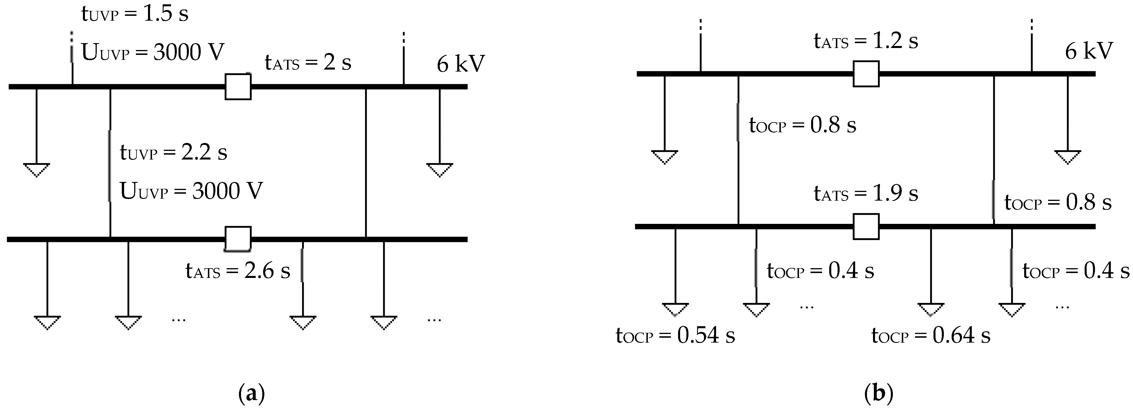
• “When the phase-to-ground voltage of the 10 kV feeder No. 1 drops below 5 kV, undervoltage protection is triggered and the power supply is disconnected. Then, the automatic transfer switch restores the supply from the feeder No. 2. Phase sequence relays installed in railway stations, GSM-Railway base stations masts and some railway level crossings also protect the equipment from voltage sags by disconnecting it when phase-to-ground voltage level drops below 90% (207 V). In stations, crossings, and substations, where automatic protection from voltage sags is not installed, the biggest problem caused by either voltage sag or supply interruption is the distortion of railway signals before the train. LED lights, metal-halide lights, various bulbs, searchlights and spotlights, heating systems of railroad switches (heating elements, magnetic starters, isolation transformers), and controllers are not very sensitive to voltage sags. Voltage, current, and earthing transformers installed in 10 kV substations are vulnerable, as well as sensitive equipment is server rooms, supervisory control and data acquisition system, teleinformation collection and transmission equipment, remote terminal units, etc.”
• “In my opinion, the impact of voltage sag must be evaluated complexly. After voltage sag, the technological process is interrupted, the equipment is disturbed, and the company suffers losses. The restart takes up to 1–4 h if there is no electronic or mechanical failure. According to monitoring data, the critical depth of voltage sag for our company is 30% of nominal phase-to-ground voltage, and the critical duration—200 ms. In case of dependent voltage sags, i.e., when two or more voltage sags occur in an interval of several seconds, the devices practically have no possibility to continue working.”
• “The technological process is interrupted after each voltage sag. Four parquet production lines are halted. Any failure of any process chain irreversibly damages unprocessed material (product). The particular sensitive part is at the end—ultraviolet coating and varnish curing. Both of these processes must be continuing. Next, voltage sags are dangerous to boiler stations. The input of biomass is inert, the forced smoke release cannot work without power supply. Moreover, the combustion continues, which poses a risk of explosion. Next, PQ impact on the grinding equipment is also dangerous because their shafts have high inertial forces. Braking is performed mechanically and electrodynamically—such facilities cannot work without power supply.”
• “The technological process is interrupted after each voltage sag, the production lines are interrupted, the restart takes up to 2 h. Particularly sensitive equipment is 0.4 kV induction motors installed in the automated lines. In the future, the company plans to install PQ monitoring equipment.”
• “Voltage sags interrupt the technological processes. Despite the fact that the appropriate protections are triggered, it does not always help, the equipment stops, and the restart is required. This generates outages, economic losses are incurred, equipment failures are caused, the quality of product suffers, production terms are prolonged.”
• “The technological process is interrupted after each voltage sag, the production lines are halted, the restart takes up to 2 h.”
• “Our company rarely experience heavy losses due to voltage sags (e.g., repair of pumps and equipment). Usually, voltage sags disrupt the process of water supply, which leads to complaints from our customers.”
• “The technological process is interrupted after each voltage sag. The equipment can be damaged. The hot water boiler stops. The restart of the equipment takes up to 2 h, sometimes longer. Moreover, the work of the network pumps is affected, and pressure fluctuations are caused. As a result, hydraulic shocks occur and the pipelines are damaged. The danger to occupational safety and health increases.”
• “When the residual voltage is equal to 0 V, the pumps and all other equipment stop. The temperature drops, the service is unavailable, the temperature schedule is not followed, direct and indirect losses are incurred, and the equipment is damaged. The likelihood of hydraulic shock increases.”
• “Particularly sensitive equipment are 0.4 kV induction motors installed in the automated lines. In the future, the company plans to install PQ monitoring equipment”.
• “We manufacture semiconductor devices. The manufacturing process is long and continuous, therefore, if any part of the chain is interrupted by voltage sag, economic losses are incurred.”
• “Voltage sags negatively affect the production of plastic and metal containers (package). When the protective relays are triggered, the plastic melting machines, metal press machines, and welding equipment stop.”
• “Voltage sags interrupt the technological process—the gas and biofuel boilers together with the electric generator stop. If the equipment is not damaged, the restoration of heat and electricity production takes 1–2 h, sometimes is longer, depending on the voltage sag depth and duration. The company suffers economic losses by not generating and not supplying both heat and electricity.”
• “The knitting and heating processes are damaged after each voltage sag. A net damaged at the knitting stage becomes waste—it cannot be sold or used for other purposes. Each time the minimum loss is EUR 600–3000 per machine (we have eight machines) plus lost time. Let us continue with the heating process—the rope stops and as a result is overheated, the impregnant is squeezed out, and the rope becomes defective. Losses—EUR 3 per meter (the length of the rope is 2000 m). In the future, the company plans to install PQ monitoring and mitigation technologies.”
• “We are a food industry company and we use modern food production equipment to produce our products. Most of the process is fully automated and is automatically stopped by the protection when voltage sag depth exceeds 10%. If at least one device is disconnected, the entire production process stops, and the production line must be cleaned before the restart. Losses depend on voltage sag magnitude, duration, location (feeder), etc., and are calculated separately in each case, but when the work efficiency is 100%, hourly losses are about EUR 22,700.”
• “We did not fill the tables for a simple reason—the voltage sags are practically undetectable without special monitoring equipment, thus only longer supply interruptions can be taken into account. The company’s losses are increasing rapidly with each passing minute. Voltage sags are particularly common in windy or adverse weather conditions. Under such conditions, the weaving looms usually cannot work.”
• “The technological process is interrupted after each voltage sag. The production lines are halted. The plastic shedders, screw loaders and centrifuges become clogged with polyethylene pieces. After each voltage sag, the plastic solidifies and must be removed from granule agglomeration units. The restart requires human resources and takes up to 4 h. Particularly sensitive equipment is the plastic film making machines. After the shutdown of the lines, a large amount of plastic waste is generated (about 4000 kg per stop). It takes up to 2–6 h to restart all the lines. It has been estimated that the company suffers a loss of EUR 5000–8000 after each dangerous voltage sag.”
• “The terminal experiences economic losses and non-material damage after voltage sag or supply interruption. After each event, the technological process is interrupted, both the operation of equipment and transport traffic are halted, and the loading process becomes unsafe and longer. The recovery takes up to several hours due to the human factor: as the person responsible for the company’s electrical sector, after a receiving a notification about the problem, I have to go to the terminal (within 4 h) and deal with the consequences outside working hours. Metal-halide lamps, which illuminate the territory, cool down and again turn on only after 30 min. Particularly sensitive equipment are computers and controllers. Some of them have UPSes. In our opinion, PQ monitoring system is not worthwhile and not cost-effective, because it only records voltage sags but does not prevent them. The monitoring, including the sharing of relevant information, must be carried out by the DSO. Most often the faults occur in the 10 kV grid, and the duration of supply interruption is equal to the automatic transfer switch time delay.”
• “The company does not have PQ analyzers or other devices; thus, we cannot provide the data about both magnitude and duration of voltage sags. Our company does not experience any significant losses due to voltage sags—the technological line is forced to stop several times a year. The restart takes up to 1 h. We do not plan to install the PQ mitigation devices as it would not be economically viable. In our opinion, more problems are caused by voltage transients. The devices are often disconnected during thunderstorms by control panels. The installed surge arresters are not efficient. In order to avoid such a problem, we stop the work by ourselves when the thunderstorm is approaching.”
• “PQ is particularly important for the production of plastic products of our company. The company has vulnerable equipment, and experiences heavy losses if the technological process is disrupted by a short circuit. There have been cases when the equipment was damaged and needed to be replaced. It usually takes two weeks from ordering new equipment parts to their replacement. Meanwhile, damaged unit is not available for use, and our company suffers heavy losses.”
• “After each voltage sag, the company suffers a loss of EUR 5000.”

The filled form is valid when at least one logically completed table is provided. In total, responses from 52 companies were taken into account. The total number of responses is given in

Table 10. Answers about MV three-phase electric motors.

Voltage, p.u.	Duration, s
	0.01 ≤ t ≤ 0.2			0.2 < t ≤ 0.5			0.5 < t ≤ 1			1 < t ≤ 5			5 < t ≤ 60
0.9 > U ≥ 0.8	7	0	4	6	1	4	3	3	5	1	1	9	1	0	10
0.8 > U ≥ 0.7	6	1	4	3	4	4	3	0	8	1	1	10	0	1	10
0.7 > U ≥ 0.4	2	3	6	1	2	8	1	1	9	0	1	10	0	1	10
0.4 > U ≥ 0.05	1	0	10	1	0	10	1	0	10	0	1	10	0	1	10
U < 0.05	1	0	10	1	0	10	1	0	10	0	1	10	0	1	10

,

Table 11. Answers about LV three-phase electric motors.

Voltage, p.u.	Duration, s
	0.01 ≤ t ≤ 0.2			0.2 < t ≤ 0.5			0.5 < t ≤ 1			1 < t ≤ 5			5 < t ≤ 60
0.9 > U ≥ 0.8	34	5	6	28	8	9	13	19	13	7	6	32	5	4	36
0.8 > U ≥ 0.7	30	8	7	12	21	12	7	10	28	3	6	36	2	4	39
0.7 > U ≥ 0.4	11	21	13	7	9	29	3	5	37	2	3	40	1	3	41
0.4 > U ≥ 0.05	10	4	31	6	3	36	2	4	39	1	4	40	1	3	41
U < 0.05	10	3	32	6	3	36	2	4	39	1	4	40	1	3	41

,

Table 12. Answers about LV single-phase electric motors.

Voltage, p.u.	Duration, s
	0.01 ≤ t ≤ 0.2			0.2 < t ≤ 0.5			0.5 < t ≤ 1			1 < t ≤ 5			5 < t ≤ 60
0.9 > U ≥ 0.8	21	2	5	20	3	5	14	7	7	9	3	16	5	5	18
0.8 > U ≥ 0.7	19	4	5	12	11	5	9	8	11	5	5	18	3	5	20
0.7 > U ≥ 0.4	12	8	8	8	7	13	6	5	17	3	4	21	1	3	24
0.4 > U ≥ 0.05	9	2	17	8	3	17	4	4	20	3	3	22	1	3	24
U < 0.05	9	2	17	7	4	17	3	5	20	3	3	22	1	3	24

,

Table 13. Answers about variable-frequency drives.

Voltage, p.u.	Duration, s
	0.01 ≤ t ≤ 0.2			0.2 < t ≤ 0.5			0.5 < t ≤ 1			1 < t ≤ 5			5 < t ≤ 60
0.9 > U ≥ 0.8	8	0	1	3	4	2	2	1	6	1	1	7	0	1	8
0.8 > U ≥ 0.7	4	4	1	1	6	2	1	0	8	0	1	8	0	0	9
0.7 > U ≥ 0.4	2	4	3	1	0	8	1	0	8	0	1	8	0	0	9
0.4 > U ≥ 0.05	2	0	7	1	0	8	1	0	8	0	0	9	0	0	9
U < 0.05	2	0	7	1	0	8	1	0	8	0	0	9	0	0	9

,

Table 14. Answers about MV three-phase generators.

Voltage, p.u.	Duration, s
	0.01 ≤ t ≤ 0.2			0.2 < t ≤ 0.5			0.5 < t ≤ 1			1 < t ≤ 5			5 < t ≤ 60
0.9 > U ≥ 0.8	1	0	0	1	0	0	0	1	0	0	1	0	0	0	1
0.8 > U ≥ 0.7	0	1	0	0	1	0	0	0	1	0	0	1	0	0	1
0.7 > U ≥ 0.4	0	1	0	0	0	1	0	0	1	0	0	1	0	0	1
0.4 > U ≥ 0.05	0	0	1	0	0	1	0	0	1	0	0	1	0	0	1
U < 0.05	0	0	1	0	0	1	0	0	1	0	0	1	0	0	1

,

Table 15. Answers about heating elements.

Voltage, p.u.	Duration, s
	0.01 ≤ t ≤ 0.2			0.2 < t ≤ 0.5			0.5 < t ≤ 1			1 < t ≤ 5			5 < t ≤ 60
0.9 > U ≥ 0.8	27	2	2	24	4	2	23	3	5	18	6	6	10	8	13
0.8 > U ≥ 0.7	27	2	2	22	5	3	21	4	6	10	11	9	7	5	19
0.7 > U ≥ 0.4	25	3	3	19	6	5	17	6	8	8	10	12	3	6	22
0.4 > U ≥ 0.05	22	4	5	19	5	7	17	4	10	4	12	15	1	4	26
U < 0.05	21	2	8	18	4	9	11	9	11	4	10	17	1	4	26

,

Table 16. Answers about controllers.

Voltage, p.u.	Duration, s
	0.01 ≤ t ≤ 0.2			0.2 < t ≤ 0.5			0.5 < t ≤ 1			1 < t ≤ 5			5 < t ≤ 60
0.9 > U ≥ 0.8	33	6	7	20	15	11	11	15	20	6	5	35	3	2	41
0.8 > U ≥ 0.7	23	13	10	10	20	16	4	16	26	1	4	41	1	1	44
0.7 > U ≥ 0.4	10	13	23	3	13	30	1	9	36	1	2	43	1	0	45
0.4 > U ≥ 0.05	5	4	37	3	2	41	0	3	43	1	2	43	1	0	45
U < 0.05	5	5	36	3	3	40	0	4	42	1	2	43	1	0	45

,

Table 17. Exceptional valid answer about controllers.

Voltage, p.u.	Duration, s
	0.01 ≤ t ≤ 0.2			0.2 < t ≤ 0.5			0.5 < t ≤ 1			1 < t ≤ 5			5 < t ≤ 60
0.9 > U ≥ 0.8	✓			✓			✓			✓			✓
0.8 > U ≥ 0.7		✓			✓			✓		✓			✓
0.7 > U ≥ 0.4			✓			✓			✓	✓			✓
0.4 > U ≥ 0.05			✓			✓			✓	✓			✓
U < 0.05		✓			✓			✓		✓			✓

,

Table 18. Answers about lighting.

Voltage, p.u.	Duration, s
	0.01 ≤ t ≤ 0.2			0.2 < t ≤ 0.5			0.5 < t ≤ 1			1 < t ≤ 5			5 < t ≤ 60
0.9 > U ≥ 0.8	31	0	1	27	4	1	24	7	1	17	6	9	12	9	13
0.8 > U ≥ 0.7	27	4	1	24	6	2	17	11	4	12	8	13	7	7	20
0.7 > U ≥ 0.4	19	8	5	16	10	6	12	10	10	9	8	16	2	7	25
0.4 > U ≥ 0.05	16	2	14	12	5	15	10	6	16	4	9	20	1	6	27
U < 0.05	15	1	16	12	3	17	7	7	19	4	7	22	1	6	27

,

Table 19. Answers about railway signals.

Voltage, p.u.	Duration, s
	0.01 ≤ t ≤ 0.2			0.2 < t ≤ 0.5			0.5 < t ≤ 1			1 < t ≤ 5			5 < t ≤ 60
0.9 > U ≥ 0.8	0	1	0	0	0	1	0	0	1	0	0	1	0	0	1
0.8 > U ≥ 0.7	0	0	1	0	0	1	0	0	1	0	0	1	0	0	1
0.7 > U ≥ 0.4	0	0	1	0	0	1	0	0	1	0	0	1	0	0	1
0.4 > U ≥ 0.05	0	0	1	0	0	1	0	0	1	0	0	1	0	0	1
U < 0.05	0	0	1	0	0	1	0	0	1	0	0	1	0	0	1

,

Table 20. Answers about servers.

Voltage, p.u.	Duration, s
	0.01 ≤ t ≤ 0.2			0.2 < t ≤ 0.5			0.5 < t ≤ 1			1 < t ≤ 5			5 < t ≤ 60
0.9 > U ≥ 0.8	12	0	6	9	3	6	7	4	7	5	1	12	2	3	13
0.8 > U ≥ 0.7	9	3	6	6	6	6	5	2	11	3	1	14	0	3	15
0.7 > U ≥ 0.4	7	1	10	5	2	11	4	1	13	2	1	15	0	1	17
0.4 > U ≥ 0.05	6	0	12	5	1	12	3	1	14	2	0	16	0	1	17
U < 0.05	6	0	12	4	2	12	3	0	15	2	0	16	0	1	17

,

Table 21. Answers about stationary computers.

Voltage, p.u.	Duration, s
	0.01 ≤ t ≤ 0.2			0.2 < t ≤ 0.5			0.5 < t ≤ 1			1 < t ≤ 5			5 < t ≤ 60
0.9 > U ≥ 0.8	2	0	0	1	1	0	1	0	1	1	0	1	0	1	1
0.8 > U ≥ 0.7	1	1	0	1	0	1	1	0	1	1	0	1	0	1	1
0.7 > U ≥ 0.4	1	0	1	1	0	1	1	0	1	1	0	1	0	0	2
0.4 > U ≥ 0.05	1	0	1	1	0	1	1	0	1	1	0	1	0	0	2
U < 0.05	1	0	1	1	0	1	1	0	1	1	0	1	0	0	2

,

Table 22. Answers about telecommunications equipment.

Voltage, p.u.	Duration, s
	0.01 ≤ t ≤ 0.2			0.2 < t ≤ 0.5			0.5 < t ≤ 1			1 < t ≤ 5			5 < t ≤ 60
0.9 > U ≥ 0.8	2	0	0	2	0	0	1	1	0	1	0	1	1	0	1
0.8 > U ≥ 0.7	2	0	0	1	1	0	1	0	1	1	0	1	0	1	1
0.7 > U ≥ 0.4	1	1	0	1	0	1	1	0	1	0	1	1	0	0	2
0.4 > U ≥ 0.05	1	0	1	1	0	1	0	1	1	0	0	2	0	0	2
U < 0.05	1	0	1	0	1	1	0	0	2	0	0	2	0	0	2

,

Table 23. Answers about welding equipment.

Voltage, p.u.	Duration, s
	0.01 ≤ t ≤ 0.2			0.2 < t ≤ 0.5			0.5 < t ≤ 1			1 < t ≤ 5			5 < t ≤ 60
0.9 > U ≥ 0.8	6	0	1	6	0	1	5	0	2	3	1	3	3	0	4
0.8 > U ≥ 0.7	6	0	1	6	0	1	4	1	2	3	1	3	0	3	4
0.7 > U ≥ 0.4	5	1	1	4	2	1	3	1	3	3	1	3	0	0	7
0.4 > U ≥ 0.05	4	1	2	4	1	2	3	0	4	3	0	4	0	0	7
U < 0.05	4	0	3	4	0	3	3	0	4	3	0	4	0	0	7

,

Table 24. Answers about automated assembly lines.

Voltage, p.u.	Duration, s
	0.01 ≤ t ≤ 0.2			0.2 < t ≤ 0.5			0.5 < t ≤ 1			1 < t ≤ 5			5 < t ≤ 60
0.9 > U ≥ 0.8	2	0	0	2	0	0	2	0	0	0	0	2	0	0	2
0.8 > U ≥ 0.7	2	0	0	2	0	0	2	0	0	0	0	2	0	0	2
0.7 > U ≥ 0.4	2	0	0	0	0	2	0	0	2	0	0	2	0	0	2
0.4 > U ≥ 0.05	2	0	0	0	0	2	0	0	2	0	0	2	0	0	2
U < 0.05	2	0	0	0	0	2	0	0	2	0	0	2	0	0	2

,

Table 25. Answers about technological process analysis and control equipment.

Voltage, p.u.	Duration, s
	0.01 ≤ t ≤ 0.2			0.2 < t ≤ 0.5			0.5 < t ≤ 1			1 < t ≤ 5			5 < t ≤ 60
0.9 > U ≥ 0.8	1	0	0	1	0	0	1	0	0	1	0	0	1	0	0
0.8 > U ≥ 0.7	1	0	0	1	0	0	1	0	0	0	1	0	0	1	0
0.7 > U ≥ 0.4	1	0	0	1	0	0	0	1	0	0	1	0	0	1	0
0.4 > U ≥ 0.05	1	0	0	1	0	0	0	1	0	0	1	0	0	1	0
U < 0.05	1	0	0	0	1	0	0	1	0	0	1	0	0	1	0

,

Table 26. Answers about autoclaves.

Voltage, p.u.	Duration, s
	0.01 ≤ t ≤ 0.2			0.2 < t ≤ 0.5			0.5 < t ≤ 1			1 < t ≤ 5			5 < t ≤ 60
0.9 > U ≥ 0.8	1	0	0	1	0	0	1	0	0	1	0	0	0	0	1
0.8 > U ≥ 0.7	1	0	0	1	0	0	1	0	0	0	1	0	0	0	1
0.7 > U ≥ 0.4	1	0	0	1	0	0	1	0	0	0	1	0	0	0	1
0.4 > U ≥ 0.05	1	0	0	1	0	0	1	0	0	0	1	0	0	0	1
U < 0.05	1	0	0	1	0	0	1	0	0	0	1	0	0	0	1

,

Table 27. Answers about vacuum coating machines.

Voltage, p.u.	Duration, s
	0.01 ≤ t ≤ 0.2			0.2 < t ≤ 0.5			0.5 < t ≤ 1			1 < t ≤ 5			5 < t ≤ 60
0.9 > U ≥ 0.8	0	1	0	0	1	0	0	0	1	0	0	1	0	0	1
0.8 > U ≥ 0.7	0	1	0	0	1	0	0	0	1	0	0	1	0	0	1
0.7 > U ≥ 0.4	0	1	0	0	1	0	0	0	1	0	0	1	0	0	1
0.4 > U ≥ 0.05	0	1	0	0	1	0	0	0	1	0	0	1	0	0	1
U < 0.05	0	1	0	0	1	0	0	0	1	0	0	1	0	0	1

,

Table 28. Answers about plastic film recycling lines, plastic pelletizing machines, and plastic film production lines.

Voltage, p.u.	Duration, s
	0.01 ≤ t ≤ 0.2			0.2 < t ≤ 0.5			0.5 < t ≤ 1			1 < t ≤ 5			5 < t ≤ 60
0.9 > U ≥ 0.8	1	0	0	1	0	0	1	0	0	1	0	0	1	0	0
0.8 > U ≥ 0.7	1	0	0	0	1	0	0	1	0	0	1	0	0	0	1
0.7 > U ≥ 0.4	0	1	0	0	0	1	0	0	1	0	0	1	0	0	1
0.4 > U ≥ 0.05	0	0	1	0	0	1	0	0	1	0	0	1	0	0	1
U < 0.05	0	0	1	0	0	1	0	0	1	0	0	1	0	0	1

and

Table 29. Answers about EV charging stations.

Voltage, p.u.	Duration, s
	0.01 ≤ t ≤ 0.2			0.2 < t ≤ 0.5			0.5 < t ≤ 1			1 < t ≤ 5			5 < t ≤ 60
0.9 > U ≥ 0.8	0	0	1	0	0	1	0	0	1	0	0	1	0	0	1
0.8 > U ≥ 0.7	0	0	1	0	0	1	0	0	1	0	0	1	0	0	1
0.7 > U ≥ 0.4	0	0	1	0	0	1	0	0	1	0	0	1	0	0	1
0.4 > U ≥ 0.05	0	0	1	0	0	1	0	0	1	0	0	1	0	0	1
U < 0.05	0	0	1	0	0	1	0	0	1	0	0	1	0	0	1

. The following color-coding is used: non-dangerous events are marked with black color, partially dangerous with orange, and dangerous with red.

The answers about electric machines are summed up in Table 10, Table 11, Table 12, Table 13 and Table 14: according to the opinion of the respondents, the closer the cell is to the upper left corner, i.e., to cell A1 (see Table 5), the less dangerous voltage sags. One company separately mentioned its electric generator. Additionally, the respondents provided the following information:

• Comments about MV three-phase electric motors:
  • “The technological process is interrupted after each voltage sag, the production lines are halted, fabrics freeze in the cutting machines, cutting defects may occur.”
  • “The company’s electric motors and variable-frequency drives are very sensitive to voltage sags.”
  • “The company’s electric motors are very sensitive to voltage sags. The company experiences losses after each dangerous voltage sag.”
  • “Voltage sags that are dangerous to 6 kV electric motors triggers the emergency automation, shifting from one power source to another for continuous energy delivery.”
• Comments about LV three-phase electric motors:
  • “The company’s electric motors are very sensitive to voltage sags.”
  • “The company’s electric motors are very sensitive to voltage sags. After each dangerous voltage sag, the company suffers a loss of about EUR 920.”
  • “No effect was observed because the motors are shut down by the automation of the control panels.”
  • “Electric motors are sensitive to voltage sags. In case of a deeper voltage sag, the company’s motors are shut down by overcurrent protection of frequency converters. It also happens that the motors without frequency converters are disconnected by the thermal protection. Supply interruption halts the production process, which restoration takes up to 1.5 h.”
  • “All company’s three-phase electric motors are sensitive to voltage sags. After each voltage sag, the company suffers economic and time losses, and a lot of manufacturing wastes are generated. The most affected workshops are knitting, thread and net dyeing, drying, and impregnation.”
  • “Short-term voltage sags do not impact the work, motors up to 100 kW operate in self-starting mode.”
  • “The company’s electric motors are very sensitive to voltage sags. After each dangerous voltage sag, the company suffers a loss of EUR 1000–11,000.”
  • “Short-term voltage sags do not have a significant impact on the work.”
  • “We cannot say exactly because we do not have PQ analyzers and we do not have any experience in voltage sag analysis.”
  • “The motors are controlled with CNC machines, and therefore are very sensitive to voltage sags. Each time we experience losses.”
  • “The electric motors of individual technological equipment are sensitive to voltage sags.”
  • “[Voltage sags] are the most dangerous for refrigeration compressors. The protection turns them off.”
  • “Electric motors are very sensitive; the company suffers a loss of EUR 5000–20,000 after each voltage sag.”
  • “Voltage sags shorten the service life of pumps, sometimes affect the impellers”.
  • “After each voltage sag (duration 200–5000 ms), the compressors disconnect and the technology stops.”
  • “Voltage sags can cause the malfunctioning of railroad switches—it is possible that the switches will not switch to the right position and, as a result, the train will be delayed.”
  • “The company’s electric motors are very sensitive to voltage sags. After each dangerous voltage sag, the company suffers a loss of about EUR 15,000.”
  • “Electric motors and servomechanisms are very sensitive to voltage sags. After each dangerous voltage sag, the company can suffer a loss of up to EUR 28,000.”
  • “The ventilation systems and pumps cease operating, resulting in production stoppage. Losses—EUR 3000 per hour.”
• Comments about LV single-phase electric motors:
  • “The effect [of voltage sags] was not noticed, because the motors are disconnected by the automation of control panels.”
  • “Voltage sags can cause the malfunctioning of railroad switches—it is possible that the switches will not switch to the right position and, as a result, the train will be delayed.”
  • “We have a large number of units that use a variety of single-phase motors. Their reactions to voltage sags are different. Each voltage sag has an impact.”
• Comments about variable-frequency drives:
  • “[Variable-frequency drives are] very sensitive [to voltage sags], because they hand or are irreparably damaged.”
  • “When voltage sag occurs, the variable-frequency drives, which tries to execute the com-mand of the controller regardless of the circumstances, stop at first. The voltage drops, the current increases until it reaches the threshold limits, and the unit fails with the overload error flag. Then, the controller stops the entire technological line.”
  • “The frequency converters are damaged if supply interruption is between 0.2 s and 2 s. If its duration is longer, the communication with controller is usually lost, which leads to the interruption of the technological process and product damage. The equipment can al-so be damaged: for example, if supply interruption occurs, ammonia [NH₃] and carbonic acid [H₂CO₃] compressors working at 100% capacity damage (crush) their filters due to the pressure, which causes 1–2 h of outage.”
  • “Longer voltage variations are dangerous to the equipment which has frequency converters. These devices stop in the case of inappropriate voltage parameters, and then need to be restarted. But before that, when the process stops, it is necessary to remove the unprocessed (raw) material that is no longer suitable for the production.”
  • “Momentary voltage variations cause voltage transients that can damage the equipment.”
  • “We cannot accurately assess the danger, because the operation of frequency converters also depends on the shape of voltage sag [e.g., single-stage or multi-stage]. The company has many frequency converters, which are sensitive to voltage sags. We suffer economic losses after each dangerous voltage sag.”
  • “When voltage variations occur, the frequency converters are disturbed, and usually are disconnected by the protection thereby protecting themself from breakdown and, as a result, disconnecting the converter-fed electric motors. In more serious situations, the frequency converters break down.”
• Comment about MV three-phase generator:
  • “After voltage sags, generator protections disconnect the generator from the power grid. The process of electricity generation is halted. Electricity is not sold.”

Contrary to electric machines, most companies acknowledge that voltage sags are not dangerous to heating elements and temperature chambers. However, in the case of a longer supply interruption, it is likely that the temperature regime will no longer be suitable for the process, for example, in the food industry. The answers about heating elements are summed up in Table 15. The following comments were received:

• “[Voltage sags] have an impact on mineral powder production.”
• “Voltage sags are not dangerous to heating elements.”
• “Temperature chambers are not sensitive to voltage sags.”
• “Heating elements are connected with semiconductor relays and thermoregulators. These devices are sensitive to voltage variations, which can interrupt their smooth operation and, in some cases, cause damage.”
• “All systems operating in the company have programmable controllers. Short-term voltage sags can freeze the controller or delete its settings (and time is wasted to reset them). Our processes are slow and do not require synchronization, thus the losses are minimal.”
• “The company’s heating elements are very sensitive to voltage sags.”
• “Heating elements are not sensitive to voltage sags; however, they are integral part of other equipment. Thus, the entire equipment stops after any dangerous PQ event.”
• “The factory is heated only with electricity. During 7 years of operation, three heater controllers failed due to voltage sags. Losses—about EUR 75. Perhaps this contributed to the breakdown of three air conditioners.”

The answers about controllers are summed up in Table 16: in this case, one exceptional response (to which the rules set in Section 3.2 do not apply) given in Table 17 was included due to solid argumentation. The following comments were received:

• “We have 13 controllers, the work of which is highly influenced by voltage sags.”
• “The company has 62 different controllers with UPSes.”
• “All production and storage equipment of the company is controlled by more than 300 controllers, and most of the 0.4 kV electric motors have frequency converters (more than 100 units in total).”
• “The company’s controllers are very sensitive to voltage sags. After each dangerous voltage sag, petrol stations stop working. We lose customers and experience losses.”
• “Controllers of two devices (out of 17) are sensitive.”
• “Some important controllers are protected with UPS; however, many smaller devices are not protected, therefore they are more sensitive to voltage sags. After the event, our employees must restore the operation of controllers and configure their settings.”
• “Most of the company’s automation equipment and controllers are sensitive to volt-age variations. Quite a few of them have double-conversion UPS, the rest is fed directly.”
• “Voltage sags have a very big influence on controllers.”
• “The controllers are fed by pulse power (output voltage is 24 VDC). The controller switches off completely after 5 s from the moment of the voltage loss, and starts without problems when the supply is restored. Obviously, the technological process is affected [by voltage sags].”
• “Controllers with pulse power supply are sensitive to voltage sags. If power source is toroidal, such controller has the immunity. We have both. We have approximately 110 machines and all of them have programmable logic controllers.”
• “Microcontrollers and electronic devices are very sensitive to voltage sags. After each dangerous voltage sag, the company can suffer a loss of up to EUR 28,000.”
• “The controllers shut down when the voltage drops below 70% with all the consequences that follow (interruption of the production process, etc.).”
• “Some controllers are very sensitive to voltage sags. The controllers must be restarted, which takes about 10 min. The company can suffer a loss of about EUR 500.”
• “The work of heating and ventilation equipment, elevators, access control systems, and traffic management systems is interrupted. The exact duration [of voltage sag] is unknown.”
• “We have 11 programmable controllers that control the temperature of our diffusion furnaces. These controllers are very sensitive to voltage sags. Depending on the situation, losses can reach up to EUR 16,000.”
• “Shorter voltage variations are dangerous, but when supply interruption is longer than 1 s, the controller restarts correctly” (see Table 17).

The answers about lighting are summed up in Table 18. It is divided into internal and territory. Inadequate lighting poses a danger to occupational safety and health. Traffic lights and railway signals can be distinguished as a separate case of the lighting (Table 19). The following comments were received:

• “We did not notice the effect [of voltage sags on lighting].”
• “We do not know exactly whether voltage sags have an effect on lighting.”
• “In case of a larger and longer voltage sag, indoor lighting turns off, but quickly recovers. Voltage sags have a greater effect on metal-halide lamps—the cool down period is required before switching on. To conclude, voltage sags have not a significant impact on lighting.”
• “In our company, the main source of lighting is various types of fluorescent lamps. In some cases, voltage stabilizers are used.”
• “The lighting usually recovers, but LED pulse power supplies often fail. This directly affect the manufacturing process and contributes to unexpected expenses.”
• “During loading, the switching off of the lighting of both the loading ramps and the territory (20 ha) poses a risk to occupational safety and health as well as increases loading time.”
• “LED power supplies are very sensitive to voltage sags. In our company, the share of LED lamps is 85%.”
• “The lighting remains working until the voltage drop is up to 50% of nominal value. If the voltage drop level is higher and the lighting is turned off, accidents are possible near the equipment in operation.”
• “Most lamps have power inverters. When the voltage drops below 50%, they turn off. This is dangerous for occupational safety and health—injuries are possible.”
• “[Voltage sags] may change railway signals: if the signal changes from allowing to stopping, train emergency braking and delay is possible.”

The answers about servers, stationary computers and telecommunications equipment are summed up in Table 20, Table 21 and Table 22. Servers are sensitive to voltage sags, but some companies answered that this can be resolved with UPSes. In the case of unexpected computer shutdown, unsaved data may be lost. In addition, some companies mentioned their communication network, for example, Profinet, an industry technical standard for data communication over Industrial Ethernet. Accordingly, it can be concluded that poor PQ is a serious obstacle to the industrial internet of things. The respondents provided the following information:

• Comments about servers:
  • “We have five servers. The installed UPS can maintain the voltage up to 8 min; therefore, a longer voltage sag is not tolerated. Each time the system reset costs up to EUR 300.”
  • “Micro and short-term power outages are dangerous [to servers] due to UPS switching delay.”
  • “Voltage sags are very dangerous to servers and can damage their electronic components.”
  • “Voltage variations disrupt our servers. They begin to conflict with each other, and their contacts may burn. Servers are very sensitive to voltage sags. The entire company’s activities are suspended while the faults are being fixed. Obviously, economic losses are experienced.”
  • “The company has a server room, the work of which is greatly affected by voltage sags.”
  • “The servers are protected with UPS. We are not afraid of voltage sags and supply interruptions that last up to 5–20 min.”
  • “We have a server room with 6 kW UPS. We had no losses due to voltage sags, and we did not register them.”
  • “Shorter voltage sags do not significantly affect the work. Our server room has UPS.”
  • “If electricity is unavailable for a longer period of time, our server room may stop.”
  • “The servers have UPS, but the switching cabinets and computer network is fed directly [from the mains].”
• Comments about stationary computers and telecommunications equipment:
  • “After a longer voltage sag, the work of stationary computers is disrupted and unsaved data is lost.”
  • “Voltage sags are very dangerous to computers, may damage electronic components.”
  • “If the computers are shut down during ship loading, the process is interrupted and data can be lost. The exact duration [of voltage sag] is unknown.”
  • “Administration work may be suspended due to computer shutdowns, although some of them are protected with UPS.”
  • “A certain part of our equipment is controlled via Profinet network. Problems with internet connection disrupts the work of factory, although most of the equipment has UPS.”

The answers about welding equipment are summed up in Table 23. In addition, two contradictory comments were received:

• “Our company has about 60 welding machines, and voltage sags greatly affect welding quality.”
• “The company’s welding and soldering equipment are resistant to voltage sags. They have no influence on the work.”

Some companies have added additional categories of equipment—automated assembly lines (Table 24), technological process analysis and control equipment (Table 25), autoclaves (Table 26), vacuum coating machines (Table 27), and plastic production equipment (Table 28). Autoclaves are used for sterilization by using high temperature pressurized steam to kill microorganisms such as bacteria, viruses, fungi, and spores on items that are placed inside. Vacuum coating is a method of creating thin protective layers on object surfaces. One company reported about the automated assembly lines that “assembly line robots are sensitive to voltage sags”, and the other reported about the autoclaves that “in the case of a longer RMS voltage variation, cases of spoilage of products cooked under high pressure are probable, the quality of the cooking is affected”.

One company separately answered about its EV charging stations, and marked all voltage sags as dangerous (see Table 29). However, it probably did this due to subjective interest in order to draw attention and press the DSO to take actions.

5. Discussion

5.1. Research Gaps

PQ impact is a broad and relevant topic not only for science but also for practice. Such studies are expected to help solve many practical problems necessary to ensure smooth economic, environmental and social development, in particular situational awareness, development of predictive maintenance systems, planning of PQ mitigation measures, power system resilience assessment and enhancement, creation of a full-fledged legal mechanism for PQ regulation, etc. The benefits, of course, can be more than just pragmatic—the search for new knowledge, the systemization of existing knowledge, as well as its dissemination are among the main tasks of science in any field.

The findings must not only be presented in the scientific literature but also transferred to standards, guidelines and other relevant documents, and the process is moving towards that. For example, it is necessary to mention IEC TR 63222-100:2023 [116], a technical report published by IEC that focuses on the impacts of PQ issues on electric equipment and power systems by collecting relevant information from CIGRÉ reports, case studies, research findings, etc., and it is hoped that the content will help users, equipment manufacturers and network operators make rational investments and actively cooperate to take specific measures for PQ improvement. Another relevant document, which complements the information given in Section 2.3, is IEC TS 60601-4-2:2024 [117], a technical specification that focuses on medical electric equipment and medical electrical systems which may fail to perform their functions because of a lack of immunity to electromagnetic disturbances. However, both documents are not freely accessible and thus cannot be reviewed in detail.

Although the subject of PQ is gradually gaining attention, the current level of research on the topic of PQ impact and its assessment is only in its early stage and far from sufficient. Also, it is not always possible to conclude whether the results of older studies are still valid. Based on the information given in Section 2 and Section 3, a framework for further research avenues on the subject of PQ impact is presented in

Table 30. A framework for the further studies on the impact of PQ.

Topic	Economic Impact	Environmental Impact	Social Impact
Influence of voltage sags on the technological (manufacturing) processes	Since technological processes are mostly sequential, each chain has a crucial role in overall reliability and thus directly correlates with the probability of causing downtime and economic losses. However, exact voltage sag immunity curves and disconnection probabilities of most electrical devices and their groups remain unknown	The operation of environmental protection equipment may be interrupted. Moreover, a sudden stoppage of some technological processes may lead to explosions	–
Influence of PQ phenomena on end-use equipment, in particular on its performance and ageing	PQ phenomena damages insulators, transformers and other electrical system elements, may trigger false protection operation. Also, they can interfere with end-use equipment. Predictive maintenance, the aging processes and many other topics currently remain open	–	Harmful electromagnetic environment can disturb vulnerable end-use devices, interfere with information-carrying signals, affect lighting. This not only results in service unavailability, but also poses a risk of wrong decision making as well as human safety and health, which directly correlates with reputational and various non-pecuniary damages
Extreme and smaller-scale events caused by weather and natural phenomena: power system resilience and the impact on grid reliability indexes	Weather-related grid faults, their impact on grid reliability as well as mitigation measures remain poorly examined. Anticipation and preparation for natural disasters is necessarily in order to at least somewhat minimize the consequences and accelerate their elimination	–	During and after natural disaster events, in addition to various problems that worsen quality of life, residents of affected areas lose power supply
Interaction between fauna, flora and electrical grid	Vegetation-related and fauna-related grid faults, their impact on grid reliability as well as the effectiveness of the applied mitigation measuresremain poorly examined, considering geographical differences of various locations	The proportion between bird collisions, electrocutions, caused PQ events, their parameters and influence on grid reliability indexes is unknown. In some cases, electrocution is able to drive population to extirpation; however, its effect on population dynamics is still unknown for most species. Also, questions such as which plant species and under what conditions can have contact with power lines, cost–benefit analysis of vegetation management, as well as utility-caused wildfires remain poorly explored	–
PQ standards and legislation: perspectives, gaps and uncertainties	EMC legislation, together with its PQ part, has a major impact on the equipment manufacturers and grid operators. A change in requirements may result in the unsuitability of existing PQ monitoring or end-use equipment and, accordingly, a need of its replacement. This will undoubtedly require new investments, may have an impact on the market. On the other hand, since PQ monitoring and mitigation are costly undertakings, the absence of requirements does not contribute to the promotion of problem solving	–	Lack of knowledge and complexity of research hinders the further development of PQ guidelines, standards and legal acts. Lack of clarity, indeterminacies, gaps and other shortcomings of PQ legislation in practice may result in different approaches, incorrect interpretation of the information or measurement results, and thus affect disputes over responsibility sharing and other issues, as well as being an obstacle in PQ monitoring planning and development of PQ assessment tools

. However, it should be noted that an understanding of what needs to be carried out on a topic of PQ impact is only a small step forward. There is a serious lack of technical capabilities for such studies: not everything can be simulated using software tools or studied in laboratories (which in turn also requires a complex and expensive set-up), whereas obtaining the results in real conditions requires long and consistent work in collecting statistics (e.g., the primary causes of grid failures, PQ event rate and their parameter distributions, etc.) and will not be fast enough simply due to the insufficient probability of occurrence of phenomena, which cannot be simply overcome with the massive installation of measuring devices due to such reasons as their functionality limitations, processing of the generated large amount of PQ data will require proper information and communication technologies (in contrast to the present, when in the absolute majority of cases PQ data are collected and analyzed manually), as well as the high cost, which will be possible to somewhat minimize when it will be feasible to solve PQ monitor allocation optimization problems in practice [1,8].

5.2. Survey as a Scientific Method

5.2.1. Surveys Conducted on the Subject of PQ

There are several previously conducted surveys on the topic of PQ in the literature, but they are older and different from the survey presented in this paper. The survey on the consequences of inadequate PQ for the Slovenian industry is given in [22] (2007). A total of 24 respondents were interviewed by adopting the questionnaire proposed by the Leonardo Power Quality Initiative (LPQI), an EU-supported educational project, and for example: (1) electric motors were identified as main sources contributing to poor PQ by 55% of respondents, followed by electronic equipment (38%), welding and smelting processes (20%), capacitor switching (17%), and processing equipment (13%); (2) 75% of respondents reported about lock-up of computers, followed by loss of synchronization of processing equipment (62.5%), data loss (58.3%), motors or other process malfunctions (45.8%), capacitor bank failure (29.2%), and nuisance tripping of relay and contactors (25%). The LPQI survey results are summarized in the final report [98] (2008): it provides information about PQ cost to the European Union economy, PQ cost components, PQ disturbances cost structure, relation between PQ cost and investments in PQ mitigation measures, responsibility sharing statistics, etc., and the data are grouped by the sectors. In total, 62 complete and 6 partial interviews were carried out, covering the following countries: Austria, France, Italy, Poland, Portugal, Slovenia, Spain, and the United Kingdom.

The PQ survey of [118] (2014) covers an even larger geography: a total of 114 grid operators (TSOs, DSOs, and the companies that operate both systems) were surveyed from all over the world—5 from Africa, 30 from the Americas, 8 from Asia, 61 from Europe, and 10 from Oceania. Despite also being a little outdated, it does not lose relevance and informativeness, and is an excellent example showing that majority voting can be a useful source of information. The answers with the most votes seem to be true compared to the PQ monitoring campaign in the Lithuanian DSO grid, for example, that the most important factor promoting PQ monitoring is consumer complaints, that the monitor used and its software have to meet the requirements of the PQ standards (e.g., according to IEC 61000-4-30:2015, the PQ events must be flagged, which undoubtedly makes the data analysis easier for the user), that grid operators usually use PQ monitoring equipment from not one but two or three different manufacturers, that the regular formal reporting is not a common practice in the world (but on the other hand, it is not very necessary and currently requires a lot of resources), etc. However, it should be noted that the questions of this survey are more related with the PQ monitoring and its planning, but not with the PQ impact assessment (see

Table 31. Highlights and analysis of the international survey of [118].

Question	Result and Discussion
Are you monitoring PQ in your network? Why do you do the monitoring?	More than 90% of respondents carry out monitoring due to customer complaints/requests, in second place is to maintain and prove standard compliance. In Lithuania, an important reason was also pressure from the National Energy Regulatory Council due to complaints from the Lithuanian Confederation of Industrialists
How many PQ monitors do you have?	This question has already been discussed in [1]. An excessive number of PQ monitors is not cost-effective, and it is impossible to monitor every power grid node. Operators use both fixed and portable monitors
How do you choose which type of monitor to use?	More than 80% of respondents answered that PQ monitor must meet the standard requirements, and more than 50% marked number of monitored channels, data output compatibility, cost, and ease of use (including both monitor and software)
What is important when you choose where to install permanent monitors?	This topic is studied in detail by [1]. Most votes were for PQ polluting (57%) and PQ sensitive (50%) customers. Some respondents mentioned their aspiration to install monitors at all HV/MV substations, or at all points of common coupling
How many different manufacturers and types of PQ monitor do you use?	The mode of answers is 2–3. The equipment (software) of different manufacturers has quite different functionality, but in essence must comply with EN 50160:2010: for instance, two different software are used in [8], and only one is able to display the entire voltage profile during the entire measurement period (but on the other hand, such functionality requires more computer resources)
Which aspects of PQ do you monitor?	Long-duration RMS voltage variations received the most votes (89%), followed by voltage sags and swells (82%), harmonics (76%), interruptions (68%), etc.
What electrical parameters do you mostly monitor?	In approximately 90% of cases, all three phases are monitored: system current is monitored by 55% of respondents, current of individual customers by 41%, phase-to-ground voltage by 85%, and phase-to-phase voltage by 50%. According to [2,8], at the moment, there is not enough experience for making sophisticated decisions from few parameters, hence it is very beneficial to have a complete picture, despite the fact that EN 50160:2010 does not require to monitor current and both voltages
How do you store the output from your monitors? How do you process the output from your monitors?	Despite the fact that computer progress over the past decade has been significantly higher than that of the PQ field, this question does not lose its relevance. Central PQ databases are used in 62% of cases, but other options, such as to store the information in separate files and distributed storage, are used as well. In most cases, the monitor-bundled software is used for PQ data analysis, but sometimes there are another but not necessarily easier options, for example, to use MS Excel. In Lithuania, manually gathered PQ data are analyzed in the bundled software and is stored in files. Further questions are related to remote data collection, duration of storage, memory size of PQ monitors—some of them have already been discussed in [1]
How often do you generate formal reports? How do you use the information?	In most cases, the formal reports are generated for the investigation of specific event, and one-third of respondents generate them regularly (weekly or monthly). Most commonly, the information is used for problem-specific internal/external reporting and PQ mitigation measures planning. During the PQ monitoring campaign in the Lithuanian DSO grid, such reports were not generated, because the purpose was technical-scientific rather than legal. Regular reporting is resource-consuming and not a common practice in the world

).

5.2.2. Limitations

Thus, considering the above, it can be affirmed that a survey is not a bad method for conducting research and analyzing information not only in social but also in technical sciences. The survey of Lithuanian industrial companies perfectly complements the information given in Section 2, and is the first work of its kind presented in the scientific literature. However, like any method, surveys also have their own limitations.

The absolute majority of the answers presented in this paper are empirical rather than rational. These answers are based on observation and experience rather than reasoning, logic and mathematics. In general, competence can be divided into four stages—this pyramid model is shown in Figure 10a and dates back to 1960s, and analogously to well-known Maslow’s pyramid (Figure 10b), the highest level cannot be reached without the lower levels. PQ is the newly emerging field [1,2,8], thus there is still a lot to be done before reaching the highest level. Undoubtedly, the primary goal of PQ research is an effective PQ mitigation strategy. The secondary could be the creation of a legal mechanism regulating the electromagnetic pollution of the grid, the practical realization of which is impossible without fully functional data collection and analysis systems. In turn, big data analysis is not possible without a comprehensive understanding of the physical nature of the PQ phenomena and AI algorithms. An insufficient level of competence poses a risk of not only both type I and type II errors but also of both type III (correct rejection of the null hypothesis but due to the wrong reason) and type IV (correct rejection of the null hypothesis but an incorrect interpretation of a correct results).

Another problem that can and does exist in both industry and science is inability (as well as reluctance) to clearly communicate available knowledge (as well as special misleading due to various subjective reasons). This can be illustrated with the Johari window (Figure 11), a visual framework divided into four quadrants that helps to understand the relationship between self and others, and, respectively, to enhance self-awareness and improve communication.

Let us roughly evaluate the competency of Lithuanian industrial companies in the various PQ subfields. The decision is presented in

Table 32. Competency evaluation of the Lithuanian industry in the field of PQ.

Aspect	Evaluation of Competence
	I	II	III	IV
Knowledge of LST EN 50160:2010	-	0.50	0.50	-
Familiarity with other PQ standards	1.00	-	-	-
Familiarity with the relevant EMC standards	1.00	-	-	-
Experience in PQ data analysis	-	0.75	0.25	-
Selection of internal monitoring nodes	-	0.50	0.50	-
Experience in remote PQ monitoring	1.00	-	-	-
Short-duration RMS variation mitigation	-	1.00	-	-
Harmonic mitigation	-	1.00	-	-
Voltage transient mitigation	1.00	-	-	-
Realization of predictive maintenance	1.00	-	-	-
Assessment of economic losses	-	0.50	0.50	-

: the maximum score in each row is 1.00, and they can be distributed only between two adjacent levels. Points are rarely given to the third level (not to mention the fourth), usually only to the first and the second. Moreover, in our opinion, the current situation in the scientific community is slightly better, but just slightly.

5.3. Further Analysis of the Survey Results: PQ Impact Similarity Assessment

In this section, possibilities of further analysis of the survey results will be demonstrated. The task is to perform a comparison in order to assess the similarly of the impact of RMS voltage variations on different end-use devices. A qualitative comparison will be performer first, followed by a quantitative comparison. The methodology is described in Section 3.2 and Section 3.3.

The comparative samples with relevant statistical parameters are listed in

Table 33. Statistical parameters of the comparative samples.

No.	Category	Size	Mean			Population Standard Deviation			Sample Standard Deviation
			1	2a	2b	1	2a	2b	1	2a	2b
1.	Controllers	46	80.22	90.71	90.61	16.94	13.52	13.67	17.12	13.57	13.72
2.	LV three-phase electric motors	44	76.05	88.00	87.88	21.09	17.46	17.56	21.33	17.66	17.76
3.	Lighting	33	48.30	65.33	65.00	25.83	25.26	25.44	26.24	25.65	25.84
4.	Heating elements	30	42.73	59.86	59.40	27.83	24.97	25.17	28.31	25.40	25.60
5.	LV single-phase electric motors	27	66.52	79.58	79.38	28.02	23.81	24.00	28.55	24.27	24.46
6.	Servers	18	72.00	83.01	82.80	29.66	23.62	23.88	30.52	24.31	24.57
7.	MV three-phase electric motors	11	80.73	89.56	89.47	23.76	20.42	20.52	24.92	21.42	21.52
8.	Variable-frequency drives	9	80.67	91.50	91.38	18.40	13.24	13.49	19.52	14.05	14.30
9.	Welding equipment	7	47.71	64.72	64.20	31.56	27.05	27.43	34.09	29.21	29.62

. The smallest sample size is 7, the largest is 46. The numbers assigned to the categories in the table will continue to be used in this work. As mentioned in Section 3, the scores are expressed as a percentage, thus the maximum value is 100, and the minimum value is 0. The samples with a size of either 1 or 2 will not be further investigated. Nevertheless, they are important for further research (e.g., end-user equipment classification) and for the general understanding of the influence of PQ on technological processes.

The type of one-tailed test in each case is given in

Table 34. Tests used for each case.

No.	1	2	3	4	5	6	7	8	9
1	-	z	z	z	t	t	t	t	t
2	z	-	z	z	t	t	t	t	t
3	z	z	-	z	t	t	t	t	t
4	z	z	z	-	t	t	t	t	t
5	t	t	t	t	-	t	t	t	t
6	t	t	t	t	t	-	t	t	t
7	t	t	t	t	t	t	-	t	t
8	t	t	t	t	t	t	t	-	t
9	t	t	t	t	t	t	t	t	-

: the z-test is used six times, and the t-test is used in the rest of the cases. The calculated scores are given in

Table 35. Scores determined using method No. 1.

No.	1	2	3	4	5	6	7	8	9
1	-	1.031	6.206	6.622	2.266	1.078	0.064	0.064	2.476
2	1.031	-	5.039	5.559	1.497	0.514	0.573	0.637	2.134
3	6.206	5.039	-	0.821	2.550	2.781	3.688	4.072	0.043
4	6.622	5.559	0.821	-	3.154	3.304	4.167	4.566	0.359
5	2.266	1.497	2.550	3.154	-	0.605	1.527	1.662	1.343
6	1.078	0.514	2.781	3.304	0.605	-	0.839	0.894	1.646
7	0.064	0.573	3.688	4.167	1.527	0.839	-	0.006	2.214
8	0.064	0.637	4.072	4.566	1.662	0.894	0.006	-	2.283
9	2.476	2.134	0.043	0.359	1.343	1.646	2.214	2.283	-

,

Table 36. Scores determined using method No. 2a.

No.	1	2	3	4	5	6	7	8	9
1	-	0.821	5.257	6.200	2.190	1.269	0.170	0.155	2.316
2	0.821	-	4.424	5.346	1.566	0.790	0.223	0.650	2.050
3	5.257	4.424	-	0.864	2.205	2.434	3.086	4.044	0.051
4	6.200	5.346	0.864	-	2.996	3.141	3.735	4.801	0.406
5	2.190	1.566	2.205	2.996	-	0.464	1.252	1.802	1.240
6	1.269	0.790	2.434	3.141	0.464	-	0.759	1.147	1.470
7	0.170	0.223	3.086	3.735	1.252	0.759	-	0.243	1.942
8	0.155	0.650	4.044	4.801	1.802	1.147	0.243	-	2.233
9	2.316	2.050	0.051	0.406	1.240	1.470	1.942	2.233	-

and

Table 37. Scores determined using method No. 2b.

No.	1	2	3	4	5	6	7	8	9
1	-	0.821	5.263	6.220	2.192	1.273	0.168	0.149	2.321
2	0.821	-	4.435	5.370	1.570	0.796	0.227	0.640	2.057
3	5.263	4.435	-	0.877	2.209	2.427	3.099	4.025	0.066
4	6.220	5.370	0.877	-	3.012	3.144	3.760	4.790	0.396
5	2.192	1.570	2.209	3.012	-	0.458	1.259	1.791	1.250
6	1.273	0.796	2.427	3.144	0.458	-	0.767	1.144	1.476
7	0.168	0.227	3.099	3.760	1.259	0.767	-	0.237	1.953
8	0.149	0.640	4.025	4.790	1.791	1.144	0.237	-	2.234
9	2.321	2.057	0.066	0.396	1.250	1.476	1.953	2.234	-

. The critical values are given in Appendix A. Obviously, the table is symmetrical with respect to the main diagonal. There are 36 tests in total. The core part of the tests is based on Equation (23). The total number of the positive decisions on the similarity are presented in

Table 38. Similarity results when the significance level is 0.05.

No.	1	2	3	4	5	6	7	8	9
1	-	3/3	0/3	0/3	0/3	3/3	3/3	3/3	0/3
2	3/3	-	0/3	0/3	3/3	3/3	3/3	3/3	0/3
3	0/3	0/3	-	3/3	0/3	0/3	0/3	0/3	3/3
4	0/3	0/3	3/3	-	0/3	0/3	0/3	0/3	3/3
5	0/3	3/3	0/3	0/3	-	3/3	3/3	1/3	3/3
6	3/3	3/3	0/3	0/3	3/3	-	3/3	3/3	3/3
7	3/3	3/3	0/3	0/3	3/3	3/3	-	3/3	0/3
8	3/3	3/3	0/3	0/3	1/3	3/3	3/3	-	0/3
9	0/3	0/3	3/3	3/3	3/3	3/3	0/3	0/3	-

,

Table 39. Similarity results when the significance level is 0.10.

No.	1	2	3	4	5	6	7	8	9
1	-	3/3	0/3	0/3	0/3	3/3	3/3	3/3	0/3
2	3/3	-	0/3	0/3	0/3	3/3	3/3	3/3	0/3
3	0/3	0/3	-	3/3	0/3	0/3	0/3	0/3	3/3
4	0/3	0/3	3/3	-	0/3	0/3	0/3	0/3	3/3
5	0/3	0/3	0/3	0/3	-	3/3	2/3	0/3	3/3
6	3/3	3/3	0/3	0/3	3/3	-	3/3	3/3	0/3
7	3/3	3/3	0/3	0/3	2/3	3/3	-	3/3	0/3
8	3/3	3/3	0/3	0/3	0/3	3/3	3/3	-	0/3
9	0/3	0/3	3/3	3/3	3/3	0/3	0/3	0/3	-

and

Table 40. Overall similarity results.

No.	1	2	3	4	5	6	7	8	9
1	-	6/6	0/6	0/6	0/6	6/6	6/6	6/6	0/6
2	6/6	-	0/6	0/6	3/6	6/6	6/6	6/6	0/6
3	0/6	0/6	-	6/6	0/6	0/6	0/6	0/6	6/6
4	0/6	0/6	6/6	-	0/6	0/6	0/6	0/6	6/6
5	0/6	3/6	0/6	0/6	-	6/6	5/6	1/6	6/6
6	6/6	6/6	0/6	0/6	6/6	-	6/6	6/6	3/6
7	6/6	6/6	0/6	0/6	5/6	6/6	-	6/6	0/6
8	6/6	6/6	0/6	0/6	1/6	6/6	6/6	-	0/6
9	0/6	0/6	6/6	6/6	6/6	3/6	0/6	0/6	-

: Table 38 presents the results when the significance level is 0.05, Table 39—when the significance level is 0.10, and Table 40—the total sum of the numbers given in Table 38 and Table 39.

It must be understood that the applied statistical method does not imply causation, thus the researcher has to figure it out by himself. The similarity of some samples can be accidental. Let us take a deeper look to all the most similar cases in order of priority:

• The similarity of “Controllers” (No. 1) with both “Servers” (No. 6) and “Variable-frequency drives” (No. 8) seems to be logical because all of them are based on printed circuit boards, but the similarity with both “LV three-phase electric motors” (No. 2) and “MV three-phase electric motors” (No. 7) cannot be explained and confirmed;
• The similarity of “LV three-phase electric motors” (No. 2) with “MV three-phase electric motors” (No. 7) and “Variable-frequency drives” (No. 8) seems very logical, but with “Servers” (No. 6) cannot be explained and confirmed;
• The similarity of “Lighting” (No. 3) with “Heating elements” (No. 4) can only be explained based on the comments of the companies, according to which voltage sags are not dangerous for both lighting and heating elements;
• The similarity of “Heating elements” (No. 4) with “Welding equipment” (No. 9) perhaps can be explained because a certain analogy can be found out in the principle of operation of these devices;
• The similarity of “LV single-phase electric motors” (No. 5) with both “Servers” (No. 6) and “Welding equipment” (No. 9) currently cannot be explained and confirmed;
• The similarity of “Servers” (No. 6) with both “MV three-phase electric motors” (No. 7) and “Variable-frequency drives” (No. 8) currently cannot be explained and confirmed;
• The similarity of “MV three-phase electric motors” (No. 7) with “Variable-frequency drives” (No. 8) seems very logical;
• The similarity of “LV single-phase electric motors” (No. 5) with “MV three-phase electric motors” (No. 7) seems very logical;
• The similarity of “LV three-phase electric motors” (No. 2) with “LV single-phase electric motors” (No. 5) seems very logical;
• The similarity of “Servers” (No. 6) with “Welding equipment” (No. 9) currently cannot be explained and confirmed;
• The similarity of “LV single-phase electric motors” (No. 5) with “Variable-frequency drives” (No. 8) currently cannot be explained and confirmed.

Next, let us proceed to the second part and quantify the similarity. Initial data are given in

Table 41. Matrices to be compared.

No.	Data	No.	Data	No.	Data
1.	$\left[\begin{array}{ccccc}21.7& 40.2& 59.8& 81.5& 91.3\\ 35.9& 56.5& 73.9& 93.5& 96.7\\ 64.1& 79.4& 88.0& 95.7& 97.8\\ 84.8& 91.3& 96.7& 95.7& 97.8\\ 83.7& 90.2& 95.7& 95.7& 97.8\end{array}\right]$	2.	$\left[\begin{array}{ccccc}18.9& 28.9& 50.0& 77.8& 84.4\\ 24.4& 50.0& 73.3& 86.7& 91.1\\ 52.2& 74.4& 87.8& 92.2& 94.4\\ 73.3& 83.3& 91.1& 93.3& 94.4\\ 74.4& 83.3& 91.1& 93.3& 94.4\end{array}\right]$	3.	$\left[\begin{array}{ccccc}3.1& 9.4& 14.1& 37.5& 51.5\\ 9.4& 15.6& 29.7& 51.5& 69.1\\ 28.1& 34.4& 46.9& 60.6& 83.8\\ 46.9& 54.7& 59.4& 74.2& 88.2\\ 51.6& 57.8& 68.2& 77.3& 88.2\end{array}\right]$
4.	$\left[\begin{array}{ccccc}9.7& 13.3& 21.0& 30.0& 54.8\\ 9.7& 18.3& 25.8& 48.3& 69.4\\ 14.5& 26.7& 35.5& 56.7& 80.7\\ 22.6& 30.7& 38.7& 67.7& 90.3\\ 29.0& 35.5& 50.0& 71.0& 90.3\end{array}\right]$	5.	$\left[\begin{array}{ccccc}21.4& 23.2& 37.5& 62.5& 73.2\\ 25.0& 37.5& 53.6& 73.2& 80.4\\ 42.9& 58.9& 69.6& 82.1& 91.1\\ 64.3& 66.1& 78.6& 83.9& 91.1\\ 64.3& 67.9& 80.4& 83.9& 91.1\end{array}\right]$	6.	$\left[\begin{array}{ccccc}33.3& 41.7& 50.0& 69.4& 80.6\\ 41.7& 50.0& 66.7& 80.6& 91.7\\ 58.3& 66.7& 75.0& 86.1& 97.2\\ 66.7& 69.4& 80.6& 88.9& 97.2\\ 66.7& 72.2& 83.3& 88.9& 97.2\end{array}\right]$
7.	$\left[\begin{array}{ccccc}36.4& 40.9& 59.1& 86.4& 90.9\\ 40.9& 54.6& 72.7& 86.4& 95.5\\ 68.2& 81.8& 86.4& 95.5& 95.5\\ 90.9& 90.9& 90.9& 95.5& 95.5\\ 90.9& 90.9& 90.9& 95.5& 95.5\end{array}\right]$	8.	$\left[\begin{array}{ccccc}11.1& 44.4& 72.2& 83.3& 94.4\\ 33.3& 55.6& 88.9& 94.4& 100.0\\ 55.6& 88.9& 88.9& 94.4& 100.0\\ 77.8& 88.9& 88.9& 100.0& 100.0\\ 77.8& 88.9& 88.9& 100.0& 100.0\end{array}\right]$	9.	$\left[\begin{array}{ccccc}14.3& 14.3& 28.6& 50.0& 57.1\\ 14.3& 14.3& 35.7& 50.0& 78.6\\ 21.4& 28.6& 50.0& 50.0& 100.0\\ 35.7& 35.7& 57.1& 57.1& 100.0\\ 42.9& 42.9& 57.1& 57.1& 100.0\end{array}\right]$

: since all elements of the matrices are expressed as a percentage of the maximum, they are the same regardless of the method (No. 1, No. 2a or No. 2b). Contrary to the first method, the second does not consider both the weights and the size of a sample, but it is not a problem.

The similarity is quantified by applying Equations (25)–(27). The calculated similarity matrices of three selected qualitatively similar pairs are given in

Table 42. Similarity matrices of several selected similar samples that can be reasoned.

Pair	Similarity
No. 1 and No. 6	${\Delta }_1=\left[\begin{array}{ccccccccc}2.5& 5.0& 5.4& 3.8& 1.3& 18.2& 25.2& 19.8& 9.8\\ 5.4& 8.0& 5.2& 2.9& 16.0& 44.4& 48.9& 37.7& 15.0\\ 8.3& 6.0& 8.3& 30.9& 54.7& 80.7& 73.5& 48.5& 16.0\\ 7.5& 7.6& 39.7& 82.3& 116.9& 127.4& 98.0& 56.0& 16.6\\ 0.7& 30.1& 77.4& 133.7& 171.8& 165.8& 117.7& 63.3& 17.2\\ 17.8& 60.7& 105.5& 148.2& 168.1& 142.5& 88.3& 41.7& 6.7\\ 31.1& 76.0& 116.3& 142.7& 150.8& 114.3& 64.4& 24.3& 1.8\\ 29.6& 65.4& 94.0& 109.2& 113.2& 80.4& 42.0& 14.4& 1.2\\ 14.2& 30.4& 42.8& 50.3& 52.3& 36.4& 19.1& 7.2& 0.6\end{array}\right]·{10}^2$
	${\Delta }_2=\left[\begin{array}{ccccccccc}3.9& 5.3& 3.1& 0.7& 3.2& 16.1& 21.6& 17.2& 8.7\\ 6.8& 6.6& 2.1& 6.2& 15.8& 38.8& 43.2& 33.7& 13.9\\ 7.2& 2.1& 11.0& 30.2& 46.7& 70.5& 65.8& 45.0& 15.6\\ 2.7& 13.9& 39.6& 71.8& 98.0& 111.4& 88.9& 53.3& 16.4\\ 5.0& 33.5& 70.8& 114.4& 146.9& 147.5& 108.8& 60.7& 17.0\\ 17.7& 53.5& 90.0& 126.3& 148.7& 131.1& 83.6& 40.7& 6.7\\ 25.9& 61.6& 95.2& 121.3& 136.4& 107.4& 62.2& 24.0& 1.8\\ 23.4& 51.5& 76.1& 93.2& 103.4& 76.0& 40.7& 14.2& 1.2\\ 11.4& 24.3& 35.4& 43.5& 48.1& 34.5& 18.5& 7.1& 0.6\end{array}\right]·{10}^2$
No. 1 and No. 8	${\Delta }_1=\left[\begin{array}{ccccccccc}2.3& 3.4& 2.0& 0.7& 2.6& 16.3& 14.7& 4.2& 2.9\\ 4.4& 5.7& 0.3& 4.5& 12.0& 32.0& 32.5& 8.2& 6.0\\ 9.6& 8.9& 3.8& 9.1& 17.9& 45.3& 35.6& 9.4& 8.2\\ 15.2& 13.5& 3.2& 5.8& 13.1& 42.7& 34.4& 15.4& 10.3\\ 20.3& 17.4& 0.9& 0.8& 6.5& 40.2& 34.0& 21.7& 12.5\\ 16.0& 13.8& 10.3& 9.3& 3.1& 20.7& 18.0& 17.5& 9.5\\ 16.9& 13.7& 25.1& 21.2& 16.8& 5.1& 0.2& 13.6& 6.4\\ 10.9& 14.9& 28.1& 21.9& 18.7& 5.3& 1.8& 12.6& 4.2\\ 5.0& 6.5& 12.5& 9.4& 7.8& 1.6& 0.4& 6.3& 2.1\end{array}\right]·{10}^2$
	${\Delta }_2=\left[\begin{array}{ccccccccc}1.2& 4.3& 4.4& 0.1& 3.6& 17.1& 15.5& 4.3& 3.0\\ 3.8& 5.7& 3.6& 5.2& 14.9& 33.0& 34.2& 8.4& 6.2\\ 7.7& 11.6& 1.6& 11.2& 19.4& 46.0& 37.1& 9.5& 8.4\\ 13.3& 13.9& 0.2& 6.1& 10.4& 43.8& 35.2& 15.7& 10.6\\ 18.0& 19.0& 1.9& 3.4& 0.7& 42.5& 34.5& 22.3& 12.8\\ 15.0& 14.5& 11.0& 12.0& 5.7& 22.3& 17.9& 18.0& 9.8\\ 15.4& 14.3& 23.1& 23.4& 16.6& 4.9& 0.7& 13.9& 6.5\\ 10.0& 14.4& 26.2& 22.5& 18.5& 6.8& 2.1& 13.0& 4.4\\ 4.6& 6.3& 11.7& 9.7& 7.7& 2.3& 0.5& 6.5& 2.2\end{array}\right]·{10}^2$
No. 2 and No. 7	${\Delta }_1=\left[\begin{array}{ccccccccc}3.3& 7.3& 13.9& 23.8& 32.3& 23.4& 17.6& 12.3& 5.5\\ 7.4& 17.3& 30.5& 45.5& 56.7& 32.8& 21.9& 16.5& 9.6\\ 16.2& 34.6& 53.1& 71.4& 84.4& 44.7& 26.4& 21.1& 10.9\\ 28.6& 54.3& 76.1& 96.8& 112.4& 55.7& 29.7& 24.2& 12.0\\ 40.8& 73.1& 96.8& 120.0& 138.0& 65.8& 32.5& 27.3& 12.9\\ 37.2& 63.0& 74.8& 85.7& 94.6& 34.9& 10.7& 13.5& 6.9\\ 33.4& 55.2& 61.8& 70.3& 74.6& 28.8& 8.0& 9.9& 2.9\\ 25.2& 39.6& 43.4& 48.4& 51.0& 19.5& 5.4& 5.9& 1.9\\ 12.3& 19.4& 21.2& 23.7& 25.0& 9.7& 2.7& 2.9& 1.0\end{array}\right]·{10}^2$
	${\Delta }_2=\left[\begin{array}{ccccccccc}6.4& 11.5& 18.5& 29.0& 37.5& 26.5& 19.5& 13.4& 5.9\\ 13.1& 22.8& 34.4& 48.9& 61.0& 34.3& 22.5& 17.2& 10.1\\ 24.5& 42.5& 57.3& 76.2& 90.0& 46.6& 26.9& 21.6& 11.2\\ 40.0& 65.1& 81.1& 102.7& 118.7& 58.0& 30.0& 25.0& 12.2\\ 54.9& 86.2& 102.1& 126.2& 145.0& 68.1& 33.0& 28.0& 13.2\\ 48.2& 72.0& 75.8& 87.7& 98.0& 35.8& 10.8& 13.8& 7.0\\ 41.7& 62.7& 62.9& 72.6& 76.7& 29.1& 8.1& 10.0& 2.9\\ 31.0& 44.7& 44.4& 49.8& 52.3& 19.8& 5.5& 6.0& 1.9\\ 15.0& 21.9& 21.7& 24.4& 25.6& 9.9& 2.8& 3.0& 1.0\end{array}\right]·{10}^2$

: after comparing the matrix No. 1 with No. 6, No. 1 with No. 8, and No. 2 with No. 7, it can be concluded that the second pair (No. 1 and No. 8) is the most similar as all values of its similarity matrices are the smallest. This could not be concluded after the qualitative test, and thus greatly expands its capabilities. At the moment, we will not focus in more depth on how to analyze these matrices or extract features from them—this is a further research avenue. One possible way to obtain a general similarity score, as suggested by [2], could be to the addition of the both similarity matrices. But perhaps the analysis could be performed in a more complex way, for example, by calculating rank, determinant, eigenvector and eigenvalues:

• The rank corresponds to the maximal number of linearly independent columns, which is equal to the maximal number of linearly independent rows. Two or more rows (columns) are called linearly independent if there is no linear expression to express their relationship with each other. The ranks of the matrices constructed from Table 6 and Table 7 is 2, and from Table 8—3. Meanwhile, the ranks of matrices given in Table 41 is 4 or 5.
• The determinant is a special number that provides a lot of useful information about the matrix. The determinant of all three matrices constructed from Table 6, Table 7 and Table 8 is equal to 0, because they all have two identical columns. Firstly, this means that the matrix does not have an inverse. Secondly, geometrically, the determinant represents the size of the region, i.e., area of parallelogram in the two-dimensional case and volume of a n-dimensional parallelotope in general case, enclosed by the vectors of matrix after a linear transformation or, in other words, linear mapping [119]: in particular, if the determinant is 0, the volume of such a parallelotope is 0, which means that it is not fully n-dimensional.
• An eigenvector is a vector with a direction that remains unchanged after a linear transformation. Such a vector is only scaled by a constant factor, which is called an eigenvalue. For instance, the matrix constructed from Table 6 has two non-zero eigenvalues—16.99 and −0.01.

5.4. Voltage Sag Tables

Such matrices, as constructed in this paper, and their properties depend not only on the values or weights of the elements, but also on both voltage and time intervals. Currently, EN 50160:2010 and IEEE Std 1564-2014 do not argue the intervals of their tables, but it can be supposed that these intervals should be somehow related with the settings of relay protection and automation, thus the absence of argumentation does not mean the absence of practical value. Indeed, one of the most important factors determining voltage sag parameters is the reaction of relay protection and automation. These devices can be divided into two groups: (1) devices that disconnect the line upon detection of improper conditions (e.g., overcurrent protection (OCP), undervoltage protection (UVP), differential protection, distance protection, zero sequence overcurrent protection, etc.), and (2) devices that automatically attempt to restore power supply after the disconnection, in particular automatic circuit recloser (ACR) and automatic transfer switch (ATS). Due to their latency and the requirement for selectivity, grid protections do not always work quickly enough as needed to protect the load from harmful effect or to prevent its downtime. Let us examine two realistic examples of the Lithuanian 6 kV grid presented in Figure 12. In order to meet the selectivity requirement, descending from a higher to a lower voltage level, ATS time settings must increase, UVP time settings must increase, and OCP time settings must decrease at any expected current value in the time–current curve. Both UVP and OCP times must be lower than the time of ATS. For example, in Figure 12a, when the depth of voltage sag is equal to 50%, one feeder will be disconnected by the UVP after 1.5 s and the ATS will be triggered after not less and usually more than 2 s, the other—after 2.2 s and ATS will be triggered after not less than 2.6 s, and such intervals can be too lengthy to maintain electric motors and other industrial equipment operating and thus to avoid outage. An effective way to speed up the operation of grid protection is installation of optical-fiber cables for signal transmission, as well as supplementation of ATS with rate of change of frequency (i.e., first time derivative of frequency) relays.

To continue, when analyzing from the PQ perspective, some traditional concepts of relay protection and automation must be expanded. Typically, all protective relays try to disconnect a PQ victim (i.e., line or device) from electricity network as soon as possible; however, some loads can be critical, thus their at least slightly longer operation can be beneficial, especially those that are used for human and environmental security (e.g., fire-fighting pumps). The purpose of relay protection and automation can not only be power system protection but also its monitoring—after transferring the parameter measurements to the operator’s data analysis system, they will be extremely useful for determining the type of fault, its location and propagation path, as well as the protection response and logical sequence [1,2]. Data collection and analysis will play a very important role in Smart Grids—absolutely correct decision making can be only achieved with knowing the whole picture, but before that, there is still a lot to be done, including the application of communication technologies and the development of AI algorithms [1,8].

Another example relates to ACR. Some grid faults disappears when the voltage is disconnected, therefore an automatic attempt to restore the power supply is beneficial and reasonable. The causes of such faults are electrical breakdown of air insulation by lightning-induced voltage transients, conductor gallop (dancing), foreign objects thrown on the lines [120], as well as the contact with flora or fauna. In addition to overhead power lines, ACR can also be and is used for the protection of busbars, power transformers, and cable lines, the failures of which often occur in air-insulated parts [120]. According to the traditional concept, from a technical point of view, ACR is considered successful when it successfully recloses the line; however, though a prism of PQ, such a successful ACR is actually unsuccessful if the electromagnetic disturbance causes consumer downtime and, respectively, worsens grid reliability indexes [2]. The success is achieved only when the consumer does not experience downtime after successful ACR, and unsuccessful ACR will in general always be a failure. When analyzing PQ measurements, it is not uncommon to find a successive voltage sag, which mostly occurs due to automation response, particularly due to reclosing events. An example of the phase-to-ground voltage measurement, which was taken in the 0.4 kV feeder of a metalworking company, which specializes in the production of forged and machined parts for the automotive industry, is given Figure 13: the time interval between the start thresholds of two observed voltage sags is 4.4 s, and a total of 3 such pairs were recorded during the month between November and December (which suggests that windy weather had an effect), which is slightly worse than the average situation in the country. However, both primary and secondary causes of such sequences (in other words, voltage sag groups or voltage sag bursts) are investigated too little—they can occur not only due to reclosing events but also due to adverse weather or incorrect registration [2,8,121]. It is noteworthy that double ACR is also sometimes used in Lithuania: in this case, according to [120], the probability of successful reclosing increases slightly (approximately 0.05–0.15), but unsuccessful reclosing damages the device.

Next, other voltage sag tables could also be used for the survey: for example, IEEE Std 1564-2014 additionally mentions the UNIPEDE table, IEC 61000-4-11 table, and IEC TR 61000-2-8 table. Their purposes are different: one tables are used for voltage sag classification, and the others for results registration during EMC tests. Therefore, one question that arises is what table should be used, and another question is time boundary values. In most tables, the shortest duration of RMS variation is equal to a half cycle, including the table of EN 50160:2010 (see Table 5). Respectively, IEC 61000-4-30:2015 requires the size of the window for voltage sag monitoring to be equal to one cycle refreshed each half cycle, which is denoted by $U_{\mathrm{R}\mathrm{M}\mathrm{S}(1/2)}$. On the other hand, IEEE Std 1159-2019 states that “sags have been defined from 2 ms (about one-eight of a cycle [at 60 Hz]) to several minutes in various publications”. The upper time limit is also not entirely clear: the time threshold of short-duration RMS variations is usually considered equal to 1 min, but the boundaries between transient, short and long interruptions have not yet been set unanimously. Regarding the voltage thresholds, the situation is much clearer: according to IEC 61000-4-30:2015, the start threshold of voltage sag is 90% of nominal grid voltage, and the end threshold is same 90% plus 2% hysteresis.

One more question, which is relevant for PQ impact assessment studies, relates to end-use equipment grouping, and perhaps a good practice of EMC standards could be useful for such a task. For example, let us examine IEC 61000-3-2:2018 [122], which limits harmonic current emissions of electrical and electronic equipment that has an input current up to and including 16 A per phase and is intended to be connected to public LV distribution systems. In this standard, the following groups are defined:

• Class A includes the equipment that is not specified as belonging to Class B, C or D, for example, balanced three-phase equipment, household appliances, vacuum cleaners, high pressure cleaners, non-portable tools, independent phase control dimmers, audio equipment, professional luminaries for stage lighting and studios;
• Class B includes portable tools and non-professional arc welding equipment;
• Class C includes lighting equipment;
• Class D includes the following types of devices if their specified power is less than or equal to 600 W: personal computers and their monitors, television receivers, and refrigerators and freezers having one or more variable-speed drives to control compressor motor(s).

Obviously, grouping of industrial equipment with higher than 16 A input current per phase is a more complicated question. Moreover, it can be carried out not only by type but also by duration of use, simultaneity of use, power consumption, frequency of use, etc. This is particularly relevant for surveys and PQ impact assessment research.

6. Conclusions

PQ impact attracts more and more attention with modern industrial development. It is a very broad topic, covering economic, environmental, and social aspects. Since PQ is a young scientific field and therefore has many research gaps [1], any comprehensive research or case study on the topic of PQ impact will have both scientific novelty and practical value. This paper not only reviewed and systemized the available literature through the prism of sustainable development, but also supplemented it by conducting a survey of Lithuanian industrial companies. In this way, the currently poor database was enlarged, encouraging foreign authors to conduct the similar or more advanced research. Further, the conclusion of this paper can be divided into two parts—engineering and mathematical:

• Currently, there is a lack of information about the impact of PQ on end-use equipment, as well as its quantification, which, for example, is essential in anticipation of predictive maintenance. In order to explore the topic, more than 60 Lithuanian industrial companies were surveyed. Although the impact can be divided into two components (equipment damage and downtime), they were not separated in the survey. The mathematical analysis of the data, the preparation of which was based on both EN 50160:2010 and IEEE Std 1564-2014, revealed the similarities between various types of equipment, but not all of them can be reasoned. Although the responses are more empirical than rational, they perfectly deepen current knowledge and lay the foundation for further research. It is not a secret that, in general, a larger and more diverse sample size can minimize survey bias and provide more representative results.
• PQ impact similarity assessment or, in the general case, comparison of datasets can be qualitative and quantitative. Applied hypothesis testing is a qualitative method. For the quantitative assessment, the convolution-based method was obtained from [2] and expanded for matrix analysis (discrete case). The qualitative method outputs the answer whether the comparative samples are similar or not, while the qualitative method does not provide such a binary response but outputs an estimate of similarity—in this way, both methods used in the ensemble perfectly complement each other. At the moment, this convolution-based method has not yet been tested with (adapted for) negative functions, oscillations, zero-crossing functions, functions with discontinuities, complex functions, multivariate functions, etc.—these cases remain for further studies.

References

1. Liubčuk, V.; Radziukynas, V.; Naujokaitis, D.; Kairaitis, G. Grid Nodes Selection Strategies for Power Quality Monitoring. Appl. Sci. 2023, 13, 6048. [Google Scholar] [CrossRef]
2. Liubčuk, V.; Radziukynas, V.; Kairaitis, G.; Naujokaitis, D. Power Quality Monitors Displacement Based on Voltage Sags Propagation Mechanism and Grid Reliability Indexes. Appl. Sci. 2023, 13, 11778. [Google Scholar] [CrossRef]
3. EN 50160:2010; Voltage Characteristics of Electricity Supplied by Public Electricity Networks. CENELEC: Brussels, Belgium, 2010.
4. IEEE Std 1159-2019; IEEE Recommended Practice for Monitoring Electric Power Quality. IEEE: New York, NY, USA, 2019.
5. European Union. Directive 2014/30/EU of the European Parliament and of the Council of 26 February 2014 on the Harmonisation of the Laws of the Member States Relating to Electromagnetic Compatibility. Off. J. Eur. Union 2014, 57, 79–105. Available online: https://eur-lex.europa.eu/legal-content/EN/TXT/?uri=CELEX%3A32014L0030 (accessed on 13 September 2024).
6. Communications Regulatory Authority of the Republic of Lithuania. Order of the RRT Director on the Approval of the Technical Regulation of Electromagnetic Compatibility. Available online: https://e-seimas.lrs.lt/portal/legalAct/lt/TAD/TAIS.289383/asr (accessed on 15 September 2024).
7. Troubleshooting Power Quality Issues in Critical Medical Diagnostic Equipment. Available online: https://www.fluke.com/en/learn/blog/power-quality/case-study-when-power-quality-is-life-or-death (accessed on 28 August 2024).
8. Liubčuk, V.; Kairaitis, G.; Radziukynas, V.; Naujokaitis, D. IIR Shelving Filter, Support Vector Machine and k-Nearest Neighbors Algorithm Application for Voltage Transients and Short-Duration RMS Variations Analysis. Inventions 2024, 9, 12. [Google Scholar] [CrossRef]
9. Lithuanian National Radio and Television. Residents of Širvintos Oppose the Wind Park: May Exterminate the Local Bird Fauna. Available online: https://www.lrt.lt/naujienos/verslas/4/2272903/sirvintiskiai-priesinasi-vejo-jegainiu-parkui-gali-isnaikinti-vietine-pauksciu-fauna (accessed on 9 September 2024).
10. Biasotto, L.D.; Kindel, A. Power Lines and Impacts on Biodiversity: A Systematic Review. Environ. Impact Assess. Rev. 2018, 71, 110–119. [Google Scholar] [CrossRef]
11. Hunters’ Thoughts on Wind Farms. Available online: https://www.medzioklezurnalas.lt/medziotoju-mintys-apie-vejo-jegainiu-parkus (accessed on 9 September 2024).
12. Bosch-Capblanch, X.; Esu, E.; Oringanje, C.M.; Dongus, S.; Jalilian, H.; Eyers, J.; Auer, C.; Meremikwu, M.; Röösli, M. The Effects of Radiofrequency Electromagnetic Fields Exposure on Human Self-Reported Symptoms: A Systematic Review of Human Experimental Studies. Environ. Int. 2024, 187, 108612. [Google Scholar]
13. World Health Organization. Radiation: Electromagnetic Fields. Available online: https://www.who.int/news-room/questions-and-answers/item/radiation-electromagnetic-fields (accessed on 16 January 2025).
14. European Communities. Council Recommendation of 12 July 1999 on the Limitation of Exposure of the General Public to Electromagnetic Fields (0 Hz to 300 GHz). Off. J. Eur. Communities 1999, 42, 59–70. Available online: https://eur-lex.europa.eu/eli/reco/1999/519/oj/eng (accessed on 16 January 2025).
15. LST EN IEC 61000-6-3:2021; Electromagnetic Compatibility (EMC)—Part 6-3: Generic Standards—Emission Standard for Equipment in Residential Environments (IEC 61000-6-3:2020). Lithuanian Standards Board: Vilnius, Lithuania, 2021.
16. LST EN IEC 61000-6-4:2019; Electromagnetic Compatibility (EMC)—Part 6-4: Generic Standards—Emission Standard for Industrial Environments (IEC 61000-6-4:2019). Lithuanian Standards Board: Vilnius, Lithuania, 2019.
17. Kivrak, E.G.; Yurt, K.K.; Kaplan, A.A.; Alkan, I.; Altun, G. Effects of Electromagnetic Fields Exposure on the Antioxidant Defense System. J. Microsc. Ultrastruct. 2017, 5, 167–176. [Google Scholar] [CrossRef]
18. Kaliatka, A. (Lithuanian Energy Institute, Kaunas, Lithuania). Personal communication, 2021.
19. Sharma, A.; Rajpurohit, B.S.; Singh, S.N. A Review on Economics of Power Quality: Impact, Assessment and Mitigation. Renew. Sustain. Energy Rev. 2018, 88, 363–372. [Google Scholar]
20. Koskolos, N.C.; Megaloconomos, S.M.; Dialynas, E.N. Assessment of Power Interruption Costs for the Industrial Customers in Greece. In Proceedings of the 8th ICHQP, Athens, Greece, 14–16 October 1998. [Google Scholar]
21. Elphick, S.; Ciufo, V.S.; Perera, S. Summary of the Economic Impacts of Power Quality on Consumers. In Proceedings of the 2015 AUPEC, Wollongong, Australia, 27–30 September 2015. [Google Scholar]
22. Kerin, U.; Dermelj, A.; Papic, I. Consequences of Inadequate Power Quality for Industrial Consumers in Slovenia. In Proceedings of the 19th CIRED, Vienna, Austria, 21–24 May 2007. [Google Scholar]
23. Avendaño, M.; Milanović, J.V.; Madrigal, M. Assessment of Financial Losses Due to Voltage Sags Using Optimal Monitoring Schemes. In Proceedings of the ICREPQ’12, Santiago de Compostela, Spain, 28–30 March 2012. [Google Scholar]
24. Perera, S.; Elphick, S. Impact and Management of Power System Voltage Sags. In Applied Power Quality; Elsevier Science: Amsterdam, The Netherlands, 2022; pp. 147–183. [Google Scholar]
25. Macangus-Gerrard, G. (Ed.) Harmonics. In Offshore Electrical Engineering Manual, 2nd ed.; Gulf Professional Publishing: Cambridge, MA, USA, 2018; pp. 273–276. [Google Scholar]
26. Fiorillo, F. Measurement and Characterisation of Magnetic Materials; Academic Press: Cambridge, MA, USA, 2004; p. 31. [Google Scholar]
27. Shokrollahi, H.; Janghorban, K. Soft Magnetic Composite Materials (SMCs). J. Mater. Process. Technol. 2007, 189, 1–12. [Google Scholar] [CrossRef]
28. Singh, P.K.; Hasan, V. Effect of Voltage Sag of Induction Motor. Int. J. Eng. Sci. Res. Technol. 2018, 7, 11–23. [Google Scholar]
29. Shareef, H.; Mohamed, A.; Marzuki, N. Analysis of Personal Computer Ride Through Capability During Voltage Sags. Electr. Power Syst. Res. 2009, 79, 1615–1624. [Google Scholar] [CrossRef]
30. Hardi, S.; Daut, I. Sensitivity of Low Voltage Consumer Equipment to Voltage Sags. In Proceedings of the 4th PEOCO, Shah Alam, Malaysia, 23–24 June 2010. [Google Scholar]
31. Wang, Y.; Dong, Y. Evaluation of Voltage Sag Severity Based on Multisource Causative Attribute. In Proceedings of the 2019 IEEE iSPEC, Beijing, China, 21–23 November 2019. [Google Scholar]
32. IEEE Std 1564-2014; IEEE Guide for Voltage Sag Indices. IEEE: New York, NY, USA, 2014.
33. SEMI F47. Available online: https://voltage-disturbance.com/voltage-quality/semi-f47-voltage-sag-immunity-standard (accessed on 7 October 2024).
34. Alshareef, S.M. Voltage Sag Assessment, Detection, and Classification in Distribution Systems Embedded with Fast Charging Stations. IEEE Access 2023, 11, 89864–89880. [Google Scholar] [CrossRef]
35. Arias-Guzman, S.; Farfan-Ustariz, A.J.; Plata, E.A.C.; Jimenez-Salazar, A.F. Implementation of IEEE Std 1564-2014 for Voltage Sag Severity Analysis on a Medium Voltage Substation. In Proceedings of the 2015 IEEE Workshop on PEPQA, Bogota, Colombia, 2–4 June 2015. [Google Scholar]
36. Ruuskanen, V.; Koponen, J.; Kosonen, A.; Hehemann, M.; Keller, R.; Niemelä, M.; Ahola, J. Power Quality Estimation of Water Electrolyzers Based on Current and Voltage Measurements. J. Power Sources 2020, 450, 227603. [Google Scholar] [CrossRef]
37. Florkowski, M.; Kuniewski, M.; Mikrut, P. Effect of Voltage Harmonics on Dielectric Losses and Dissipation Factor Interpretation in High-Voltage Insulating Materials. Electr. Power Syst. Res. 2024, 226, 109973. [Google Scholar]
38. LST EN IEC 61800-3:2023; Adjustable Speed Electrical Power Drive Systems—Part 3: EMC Requirements and Specific Test Methods for PDS and Machine Tools. Lithuanian Standards Board: Vilnius, Lithuania, 2023.
39. LST EN IEC 61000-2-4:2024; Electromagnetic Compatibility (EMC)—Part 2-4: Environment—Compatibility Levels in Power Distribution Systems in Industrial Locations for Low-Frequency Conducted Disturbances. Lithuanian Standards Board: Vilnius, Lithuania, 2024.
40. Boльдeк, A.И. Элeктpичecкиe Maшины, 3rd ed.; Toлвинcкaя, E.B., Ed.; «Энepгия»: Leningrad, Russia, 1978. [Google Scholar]
41. Kemabonta, T.; Mowry, G. A Syncretistic Approach to Grid Reliability and Resilience: Investigations from Minnesota. Energy Strat. Rev. 2021, 38, 100726. [Google Scholar] [CrossRef]
42. Kenward, A.; Raja, U. Blackout: Extreme Weather, Climate Change and Power Outages; Climate Central: Princeton, NJ, USA, 2014; Available online: http://assets.climatecentral.org/pdfs/PowerOutages.pdf (accessed on 7 February 2025).
43. Potts, J.; Tiedmann, H.R.; Stephens, K.K.; Faust, K.M.; Castellanos, S. Enhancing Power System Resilience to Extreme Weather Events: A Qualitative Assessment of Winter Storm Uri. Int. J. Disaster Risk Reduct. 2024, 103, 104309. [Google Scholar] [CrossRef]
44. Harness, R.E.; Juvvadi, P.R.; Dwyer, J.F. Avian Electrocutions in Western Rajasthan, India. J. Raptor Res. 2023, 47, 352–364. [Google Scholar] [CrossRef]
45. Harness, R.; Gombobaatar, S.; Yosef, R. Mongolian Distribution Power Lines and Raptor Electrocutions. In Proceedings of the 2008 IEEE Rural Electric Power Conference, Charleston, SC, USA, 27–29 April 2008. [Google Scholar]
46. Galis, M.; Nad’o, L.; Hapl, E.; Šmídt, J.; Deutschová, L.; Chavko, J. Comprehensive Analysis of Bird Mortality along Power Distribution Lines in Slovakia. Raptor J. 2019, 13, 1–25. [Google Scholar] [CrossRef]
47. Hamal, S.; Sharma, H.P.; Gautam, R.; Katuwal, H.B. Drivers of Power Line Collisions and Electrocutions of Birds in Nepal. Ecol. Evol. 2023, 13, 10080. [Google Scholar] [CrossRef]
48. Raptor Protection of Slovakia. Electrocutions & Collisions of Birds in EU Countries: The Negative Impact & Best Practices for Mitigation—An Overview of Previous Efforts and Up-to-Date Knowledge of Electrocutions and Collisions of Birds Across 27 EU Member States; Raptor Protection of Slovakia: Bratislava, Slovakia, 2021; Available online: https://www.birdlife.org/wp-content/uploads/2022/10/Electrocutions-Collisions-Birds-Best-Mitigation-Practices-NABU.pdf (accessed on 9 February 2025).
49. Bald Eagle Comes to Chicago, Gets Electrocuted on a Power Line. Available online: https://www.dnainfo.com/chicago/20160303/midway/chicago-bald-eagle-that-got-electrocuted-on-southwest-side-power-line (accessed on 11 September 2024).
50. Bald Eagle Electrocuted in Power Line Crash, 145 Residents Lose Power. Available online: https://mynorthwest.com/3945731/bald-eagle-electrocuted-power-line-crash-145-residents-lose-power (accessed on 11 September 2024).
51. YouTube. Leopard Climbs Electric Pole, Gets Electrocuted [Video]. Available online: https://www.youtube.com/watch?v=5iRbqKfh3TY (accessed on 11 September 2024).
52. The Guardian. Elephants Electrocuted by Sagging Power Lines. Available online: https://www.theguardian.com/environment/india-untamed/2015/sep/15/elephants-electrocuted-by-sagging-power-lines (accessed on 11 September 2024).
53. The Hindu. Wild Elephant Electrocuted After Power Line Falls on it Near Coimbatore. Available online: https://www.thehindu.com/news/cities/Coimbatore/wild-elephant-electrocuted-dies-after-power-line-falls-on-it-near-coimbatore/article66660290.ece (accessed on 11 September 2024).
54. The Telegraph. High-Tension Wire Kills Python. Available online: https://www.telegraphindia.com/west-bengal/high-tension-wire-kills-python/cid/1572066 (accessed on 11 September 2024).
55. Hernández-Matías, A.; Real, J.; Parés, F.; Pradel, R. Electrocution Threatens the Viability of Populations of the Endangered Bonelli’s Eagle (Aquila fasciata) in Southern Europe. Biol. Conserv. 2015, 191, 110–116. [Google Scholar] [CrossRef]
56. Installation of the Bird Protection Measures on the High Voltage Electricity Transmission Grid in Lithuania. Final Report. 2019. Available online: http://www.birds-electrogrid.lt/news/159/208/European-Commission-has-approved-the-final-LIFE-Birds-on-Electrogrid-report/d,detalus-en (accessed on 14 February 2025).
57. Installation of Bird Collision Mitigation Measures in Bird Staging Areas. Available online: http://www.birds-electrogrid.lt/en/conservation-actions/installation-of-bird-collision-mitigation-measures-in-bird-staging-areas-c1 (accessed on 14 February 2025).
58. Installation of Line Markers in the Most Sensitive Areas. Available online: http://www.birds-electrogrid.lt/en/conservation-actions/installation-of-line-markers-in-the-most-sensitive-areas-c2 (accessed on 14 February 2025).
59. Installation of Bird Protection Measures on the Utility Poles. Available online: http://www.birds-electrogrid.lt/en/conservation-actions/installation-of-bird-protection-measures-on-the-utility-poles-c3 (accessed on 14 February 2025).
60. Erecting of Nest-Boxes for Falcons. Available online: http://www.birds-electrogrid.lt/en/conservation-actions/erecting-of-nest-boxes-for-falcons-c4 (accessed on 14 February 2025).
61. Ex Ante and Post Ante Monitoring on the Effectiveness of the Project Conservation Actions (2014–2015). Activity Report. 2016. Available online: http://www.birds-electrogrid.lt/news/55/187/The-report-on-D2-acivity-Ex-ante-and-post-ante-monitoring-on-the-effectiveness-of-the-project-conservation-actions-was-prepared/d,detalus-en (accessed on 14 February 2025).
62. Infante, O.; Peris, S. Bird Nesting on Electric Power Supports in Northwestern Spain. Ecol. Eng. 2003, 20, 321–326. [Google Scholar] [CrossRef]
63. Barauskas, R.; Karlonas, M. Lietuvos Paukščiai: Perinčios ir Kasmet Aptinkamos Rūšys, 2nd ed.; Lututė: Kaunas, Lithuania, 2023. [Google Scholar]
64. Komsomolskaya Pravda. A Bear and a Fox were Killed by a Powerful Electric Shock in the Taiga in Kolyma. Available online: https://www.hab.kp.ru/daily/28302.5/4442350 (accessed on 11 September 2024).
65. BBC. Kruger National Park Electrocution Kills Six Big Animals. Available online: https://www.bbc.com/news/world-africa-47047889 (accessed on 11 September 2024).
66. Foxes Die on Power Lines. Impact of the War in Ukraine. Available online: https://www.medzioklezurnalas.lt/lapes-mirsta-ant-elektros-liniju-karo-poveikis-ukrainoje (accessed on 12 September 2024).
67. EKO-Inform [Facebook Page]. Not for the Weak Nerves [Video]. Available online: https://www.facebook.com/reel/430597682687105 (accessed on 12 September 2024).
68. Marxen, T. New Technology to Cut Victoria’s Powerline Fire Risk. In Proceedings of the Arboriculture Australia National Conference 2016, Melbourne, Australia, 23 February 2016. [Google Scholar]
69. Babrauskas, V. Electricity-Caused Wildland Fires: Costs, Social Fairness, and Proposed Solution. Fire 2024, 7, 442. [Google Scholar] [CrossRef]
70. Kandanaarachchi, S.; Anantharama, N.; Muñoz, M.A. Early Detection of Vegetation Ignition Due to Powerline Faults. IEEE Trans. Power Deliv. 2020, 36, 1324–1334. [Google Scholar] [CrossRef]
71. Bandara, S.; Rajeev, P.; Gad, E. Power Distribution System Faults and Wildfires: Mechanisms and Prevention. Forests 2023, 14, 1146. [Google Scholar] [CrossRef]
72. Coldham, D.; Czerwinski, A.; Marxsen, T. Probability of Bushfire Ignition from Electric Arc Faults; HRL Technology: Melbourne, Australia, 2011. [Google Scholar]
73. Seimas of the Republic of Lithuania. Law of the Republic of Lithuania on Special Conditions of Land Use. Available online: https://e-seimas.lrs.lt/portal/legalAct/lt/TAD/46c841f290cf11e98a8298567570d639/asr (accessed on 9 February 2025).
74. Smith, M.B.; Aborn, D.A.; Gaudin, T.J.; Tucker, J.C. Mammalian Predator Distribution Around a Transmission Line. Southeast. Nat. 2008, 7, 289–300. [Google Scholar]
75. Rieucau, G.; Vickery, W.L.; Doucet, G.J. A Patch Use Model to Separate Effects of Foraging Costs on Giving-up Densities: An Experiment with White-Tailed Deer (Odocoileus virginianus). Behav. Ecol. Sociobiol. 2009, 63, 891–897. [Google Scholar]
76. Bartzke, G.; May, R.F.; Bevanger, K.M.; Stokke, S.; Røskaft, E. The Effects of Power Lines on Ungulates and Implications for Power Line Routing and Rights-of-Way Management. Int. J. Biodivers. Conserv. 2014, 6, 647–662. [Google Scholar]
77. Barauskas, R.; Babelis, D. Lietuvos Žinduoliai: Išvaizda, Paplitimas, Buveinės, Gyvenimo Būdas, Veiklos Žymės; Lututė: Kaunas, Lithuania, 2025. [Google Scholar]
78. Hernanz, J.A.R.; Martín, J.J.C.; Gogeascoechea, J.C.; Belver, I.Z. Insulator Pollution in Transmission Lines. REPQJ 2006, 4, 124–130. [Google Scholar]
79. Hadipour, M.; Shiran, M.A. Various Pollutions of Power Lines Insulators. Majlesi J. Energy Manag. 2017, 6, 29–38. [Google Scholar]
80. Gençoğlu, M.T.; Cebeci, M. Investigation of Pollution Flashover on High Voltage Insulators Using Artificial Neural Network. Expert Syst. Appl. 2009, 36, 7338–7345. [Google Scholar] [CrossRef]
81. Mao, X.; Ye, J.; Tian, Z.; Hu, K.; Wang, J.; Tan, F. Study on the Flashover Mechanism of Bird Droppings in the Transmission Line. AIP Adv. 2023, 13, 105204. [Google Scholar] [CrossRef]
82. Electrical Engineering Portal. How Arc Suppression Reactors (Earth Fault Neutralizers or Petersen-Coils) Work? Available online: https://electrical-engineering-portal.com/arc-suppression-reactors (accessed on 10 March 2025).
83. Ministry of Energy of the Republic of Lithuania. Order of the Minister of Energy of the Republic of Lithuania on the Approval of the Rules for the Supply and Use of Electricity. Available online: https://e-seimas.lrs.lt/portal/legalAct/lt/TAD/TAIS.365540/asr (accessed on 4 February 2025).
84. IEEE Std 519-2022; IEEE Standard for Harmonic Control in Electric Power Systems. IEEE: New York, NY, USA, 2022.
85. LST EN 61000-2-2:2003; Electromagnetic Compatibility (EMC)—Part 2-2: Environment—Compatibility Levels for Low-Frequency Conducted Disturbances and Signaling in Public Low-Voltage Power Supply Systems. Lithuanian Standards Board: Vilnius, Lithuania, 2003.
86. LST EN 61000-4-7:2004; Electromagnetic Compatibility (EMC)—Part 4-7: Testing and Measurement Techniques—General Guide on Harmonics and Interharmonics Measurements and Instrumentation, for Power Supply Systems and Equipment Connected Thereto. Lithuanian Standards Board: Vilnius, Lithuania, 2004.
87. LST EN 61000-4-15:2011; Electromagnetic Compatibility (EMC)—Part 4-15: Testing and Measurement Techniques—Flickermeter—Functional and Design Specifications. Lithuanian Standards Board: Vilnius, Lithuania, 2011.
88. LST EN 61000-4-30:2015; Electromagnetic Compatibility (EMC)—Part 4-30: Testing and Measurement Techniques—PQ Measurement Methods. Lithuanian Standards Board: Vilnius, Lithuania, 2016.
89. Council of European Energy Regulators. 5th CEER Benchmarking Report on the Quality of Electricity and Gas Supply; CEER: Brussels, Belgium, 2011. [Google Scholar]
90. Ström, L.; Bollen, M.H.J.; Kolessar, R. Voltage Quality Regulation in Sweden. In Proceedings of the 21th CIRED, Frankfurt, Germany, 6–9 June 2011. [Google Scholar]
91. Torkzadeh, R.; Waes, J.; Ćuk, V.; Cobben, S. Model Validation for Voltage Dip Assessment in Future Networks. Electr. Power Syst. Res. 2023, 217, 109099. [Google Scholar] [CrossRef]
92. Council of European Energy Regulators. 7th CEER Benchmarking Report on the Quality of Electricity and Gas Supply; CEER: Brussels, Belgium, 2022. [Google Scholar]
93. ANSI C84.1-2016; Electric Power Systems and Equipment—Voltage Ratings (60 Hertz). ANSI: Washington, DC, USA, 2016.
94. Voltage Fluctuations, Flicker and Power Quality. Available online: https://www.fluke.com/en/learn/blog/power-quality/voltage-fluctuations-flicker (accessed on 12 September 2024).
95. Why Is Good Power Quality Crucial in Data Centers? Available online: https://meruspower.com/blog/good-power-quality-crucial-data-centers (accessed on 9 September 2024).
96. Siostrzonek, T.; Wójcik, J.; Dutka, M.; Siostrzonek, W. Impact of Power Quality on the Efficiency of the Mining Process. Energies 2024, 17, 5675. [Google Scholar] [CrossRef]
97. Bhattacharyya, S.; Cobben, S. Consequences of Poor Power Quality—An Overview. In Power Quality; Eberhard, A., Ed.; IntechOpen: London, UK, 2011; pp. 3–24. [Google Scholar]
98. Manson, J.; Targosz, R. Leonardo ENERGY—European Power Quality Survey Report; International Copper Association Europe: Brussels, Belgium, 2008; Available online: https://www.slideshare.net/slideshow/european-power-quality-survey-report/149087013 (accessed on 21 February 2025).
99. Hartungi, R.; Jiang, L. Investigation of Power Quality in Health Care Facility. In Proceedings of the ICREPQ’10, Granada, Spain, 23–25 March 2010. [Google Scholar]
100. The Critical Role of Power Supply in Medical Imaging and Diagnostic Equipment. Available online: https://www.horizon-pss.com/news-events/blog-the-critical-role-of-power-supply-in-medical-imaging-and-diagnostic-equipment (accessed on 19 February 2025).
101. Ramos, M.C.G.; Tahan, C.M.V. An Assessment of the Electric Power Quality and Electrical Installation Impacts on Medical Electrical Equipment Operations at Health Care Facilities. Am. J. Appl. Sci. 2009, 6, 638–645. [Google Scholar] [CrossRef]
102. Rao, U.; Singh, S.N.; Thakur, C.K. Power Quality Issues with Medical Electronics Equipment in Hospitals. In Proceedings of the 2010 International Conference on Industrial Electronics, Control and Robotics, Rourkela, India, 27–29 December 2010. [Google Scholar]
103. Moreira, A.C.; Silva, L.C.P.; Paredes, H.K.M. Electrical Modelling and Power Quality Analysis of Three-Phase X-Ray Apparatus. In Proceedings of the SPEEDAM 2014, Ischia, Italy, 18–20 June 2014. [Google Scholar]
104. Takla, G.M.S.; Petre, J.H.; Doyle, D.J.; Horibe, M.; Gopakumaran, B. The Problem of Artifacts in Patient Monitor Data During Surgery: A Clinical and Methodological Review. Anesth. Analg. 2006, 103, 1196–1204. [Google Scholar] [CrossRef]
105. Buzdugan, M.I.; Bălan, H.; Mureşan, D.T. An Electrical Power Quality Problem in an Emergency Unit from a Hospital—Case Study. In Proceedings of the SPEEDAM 2010, Pisa, Italy, 14–16 June 2010. [Google Scholar]
106. Hanada, E.; Itoga, S.; Takano, K.; Kudou, T. Investigations of the Quality of Hospital Electric Power Supply and the Tolerance of Medical Electric Devices to Voltage Dips. J. Med. Syst. 2007, 31, 219–233. [Google Scholar] [CrossRef]
107. Hanada, E.; Kudou, T. Electromagnetic Noise in the Clinical Environment. In Proceedings of the ISMICT2009, Montreal, QC, Canada, 24–26 February 2009. [Google Scholar]
108. Neves Neto, J.C.; Almeida, C.F.M.; Delbone, E.; Starosta, J. Investigation of Harmonic Resonance from Reactive Compensation in Hospital Electrical Installations with Magnetic Resonance Imaging (MRI). In Proceedings of the 20th ICHQP, Naples, Italy, 29 May–1 June 2022. [Google Scholar]
109. Özdemirci, E.; Yatak, M.Ö.; Duran, F.; Canal, M.R. Reliability Assessment of Infant Incubator and the Analyzer. Gazi Univ. J. Sci. 2014, 27, 1169–1175. [Google Scholar]
110. Ishida, K.; Hirose, M.; Hanada, E. Investigation of Interference with Medical Devices by Power Line Communication to Promote its Safe Introduction to the Clinical Setting. In Proceedings of the 2016 International Symposium on Electromagnetic Compatibility—EMC Europe, Wroclaw, Poland, 5–9 September 2016. [Google Scholar]
111. Mariappan, P.M.; Raghavan, D.R.; Aleem, S.H.E.A.; Zobaa, A.F. Effects on Electromagnetic Interference on the Functional Usage of Medical Equipment by 2G/3G/4G Cellular Phones: A Review. J. Adv. Res. 2016, 7, 727–738. [Google Scholar] [CrossRef]
112. Radvilė, E.; Urbonas, R. Digital Transformation in Energy Systems: A Comprehensive Review of AI, IoT, Blockchain, and Decentralised Energy Models. Energetika 2025, 71, 1–22. [Google Scholar] [CrossRef]
113. Faheem, M.; Shah, S.; Bytt, R.; Raza, B.; Anwar, M.; Ashraf, M.; Ngadi, M.; Gungor, V. Smart Grid Communication and Information Technologies in the Perspective of Industry 4.0: Opportunities and Challenges. Comput. Sci. Rev. 2018, 30, 1–30. [Google Scholar]
114. Stanelytė, D.; Radziukynienė, N.; Radziukynas, V. Overview of Demand-Response Services: A Review. Energies 2022, 15, 1659. [Google Scholar] [CrossRef]
115. Montgomery, D.C.; Runger, G.C. Applied Statistics and Probability for Engineers, 5th ed.; John Wiley & Sons: Hoboken, NJ, USA, 2011. [Google Scholar]
116. IEC TR 63222-100:2023; Power Quality Management—Part 100: Impact of Power Quality Issues on Electrical Equipment and Power System. IEC: Geneva, Switzerland, 2023.
117. IEC TS 60601-4-2:2024; Medical Electrical Equipment—Part 4-2: Guidance and Interpretation—Electromagnetic Immunity: Performance of Medical Electrical Equipment and Medical Electrical Systems. IEC: Geneva, Switzerland, 2024.
118. Milanovic, J.V.; Meyer, J.; Ball, R.F.; Howe, W.; Preece, R.; Bollen, M.H.J.; Elphick, S.; Cukalevski, N. International Industry Practice on Power Quality Monitoring. IEEE Trans. Power Deliv. 2014, 29, 934–941. [Google Scholar]
119. YouTube. The Determinant [Video]. Available online: https://www.youtube.com/watch?v=Ip3X9LOh2dk&list=PLZHQObOWTQDPD3MizzM2xVFitgF8hE_ab&index=7 (accessed on 4 November 2024).
120. Svinkūnas, G.; Navickas, A. Elektros Energetikos Pagrindai, 2nd ed.; Kaunas University of Technology—Publishing House “Technologija”: Kaunas, Lithuania, 2013. [Google Scholar]
121. De Santis, M.; Di Stasio, L.; Noce, C.; Varilone, P.; Verde, P. Indices of Intermittence to Improve the Forecasting of the Voltage Sags Measured in Real Systems. IEEE Trans. Power Deliv. 2021, 37, 1252–1263. [Google Scholar]
122. LST EN IEC 61000-3-2:2019; Electromagnetic Compatibility (EMC)—Part 3-2: Limits—Limits for Harmonic Current Emissions (Equipment Input Current ≤ 16 A per Phase). Lithuanian Standards Board: Vilnius, Lithuania, 2020.
Figure 1. (a) Essential requirements for the electromagnetic compatibility of equipment. (b) Principal groups of the electromagnetic emissions.
Inventions 10 00030 g001
Figure 2. A look at PQ through the prism of sustainable development.
Inventions 10 00030 g002
Figure 3. Test results of the LV single-phase equipment immunity to short-duration RMS voltage variations provided by [24,29,30]. During the tests, the operation of the devices was not disrupted by the RMS variations above the curve and vice versa.
Inventions 10 00030 g003
Figure 4. Comparison of EN 50160:2010 voltage harmonic levels (up to the 25th) with IEC 61800-3:2022 immunity requirements (up to the 40th). The absence of a column means that there is no requirement—it is under consideration and therefore not yet given.
Inventions 10 00030 g004
Figure 5. Fauna of Lithuania in the spring of 2024. (a) White stork (Ciconia ciconia); (b) Red fox (Vulpes vulpes); (c) European moose (A. alces alces).
Inventions 10 00030 g005
Figure 6. (a) Phase-to-phase and (b) phase-to-ground voltages in the 330 kV 100 km line at the generator’s terminals where a two-phase-to-ground fault occurs obtained by [2] during the simulation (Scenario No. 1, two-phase-to-ground fault, voltage at the monitor M1). Currently, it is not clear which array—one phase-to-phase supply interruption with two 50% depth voltage sags or two phase-to-ground supply interruptions with a 10% depth voltage sag—is more favorable to the operator from the juridical point of view.
Inventions 10 00030 g006
Figure 7. (a) Phase-to-phase and (b) phase-to-ground voltages at the end of the 330 kV 100 km line when a two-phase fault occurs at the generator’s terminals in the beginning of this 100 km line obtained by [2] during the simulation (Scenario No. 1, two-phase fault, voltage at the monitor M2). Currently, it is not clear which array—one phase-to-phase supply interruption with two 10% depth voltage sags or one healthy phase-to-ground voltage with two 50% depth voltage sags—is more favorable to the operator from the juridical point of view.
Inventions 10 00030 g007
Figure 8. (a) Phase-to-phase and (b) phase-to-ground voltages in the 10 kV line where a single-phase fault occurs obtained by [2] during the simulation (Scenario No. 3, single-phase fault, voltage at the monitor M2a). It is clear that this fault will not be noticed if only phase-to-phase voltage is taken into consideration, as is required by EN 50160:2010.
Inventions 10 00030 g008
Figure 9. An example of the system architecture of advanced metering infrastructure and its integration with PQ and other necessary Smart Grid applications [113].
Inventions 10 00030 g009
Figure 10. (a) The four stages of competence; (b) Maslow’s hierarchy of needs.
Inventions 10 00030 g010
Figure 11. The Johari window.
Inventions 10 00030 g011
Figure 12. Realistic examples of the settings of relay protection and automation, which have a direct influence on the parameters of short-duration RMS variations, their impact on the load and consequences. (a) A combination of UVP and ATS; (b) A combination of OCP and ATS.
Inventions 10 00030 g012
Figure 13. Two dependent phase-to-ground voltage sags (occurred on 24 November 2023) in the 0.4 kV feeder of the metalworking plant (located in Marijampolė municipality). The time interval between their start thresholds is 4.4 s.
Inventions 10 00030 g013