Article

Homotopy Semi-Numerical Modeling of Non-Newtonian Nanofluid Transport External to Multiple Geometries Using a Revised Buongiorno Model

1
Department of Mathematics, Motilal Nehru National Institute of Technology Allahabad, Prayagraj 211004, India
2
Department of Mechanical and Aeronautical Engineering, Salford University, Salford M54WT, UK
3
Department of Mechanical Engineering, Cleveland State University, Cleveland, OH 44115-2214, USA
4
Department of Mathematics, Indian Institute of Technology Kharagpur, Kharagpur 721302, India
*
Authors to whom correspondence should be addressed.
Inventions 2019, 4(4), 54; https://doi.org/10.3390/inventions4040054
Submission received: 20 August 2019 / Revised: 16 September 2019 / Accepted: 20 September 2019 / Published: 25 September 2019
(This article belongs to the Special Issue Recent Trends in Nanofluids)

Abstract

:
A semi-analytical solution for the convection of a power-law nanofluid external to three different geometries (i.e., cone, wedge and plate), subject to convective boundary condition is presented. A revised Buongiorno model is employed for the nanofluid transport over the various geometries with variable wall temperature and nanoparticle concentration conditions (non-isothermal and non-iso-solutal). Wall transpiration is included. The dimensional governing equations comprising the conservation of mass, momentum, energy and nanoparticle volume fraction are transformed to dimensionless form using appropriate transformations. The transformed equations are solved using a robust semi-analytical power series method known as the Homotopy analysis method (HAM). The convergence and validation of the series solutions is considered in detail. The variation of order of the approximation and computational time with respect to residual errors for temperature for the different geometries is also elaborated. The influence of thermophysical parameters such as wall temperature parameter, wall concentration parameter for nanofluid, Biot number, thermophoresis parameter, Brownian motion parameter and suction/blowing parameter on the velocity, temperature and nanoparticle volume fraction is visualized graphically and tabulated. The impact of these parameters on the engineering design functions, e.g., coefficient of skin fraction factor, Nusselt number and Sherwood number is also shown in tabular form. The outcomes are compared with the existing results from the literature to validate the study. It is found that thermal and solute Grashof numbers both significantly enhance the flow velocity whereas they suppress the temperature and nanoparticle volume fraction for the three different configurations, i.e., cone, wedge and plate. Furthermore, the thermal and concentration boundary layers are more dramatically modified for the wedge case, as compared to the plate and cone. This study has substantial applications in polymer engineering coating processes, fiber technology and nanoscale materials processing systems.

1. Introduction

The Convective flow over different geometrical configurations (e.g., wedge, cone, plate) arises in a diverse spectrum of engineering systems including polymer engineering, fiber technology, geothermal transport in the vicinity of rock formations, thermal-aerodynamics of high-speed flight, nuclear cooling systems, spray deposition techniques, coating and surface treatment, etc. Numerous studies have been communicated in this regard using both analytical and computational methods for multiple geometries and for both Newtonian and non-Newtonian fluids. Roy [1] studied the natural convection from vertical cone at high Prandtl number. Vajravelu and Nayfeh [2] inspected the effect of heat generation or absorption on the flow and heat transfer along the surface of a cone under magnetohydrodynamics (MHD) effects. Natural convection from a wedge and cone subject to mixed thermal boundary conditions has been addressed by Ramanaiah and Malaryizhi [3]. Watanabe et al. [4] have analyzed the response of mixed convection boundary layer flow over a wedge to the effect of surface transpiration, i.e., suction/blowing. Fang and Lee [5] considered the flow of rarefied gas free stream over a moving flat plate. Xu and Liao [6] discussed the flow and heat transfer of an Ostwald-De Waele power-law fluid over a stretching flat plate. Natural convection heat and mass transfer from a vertical cone in a porous medium with variable wall concentration was analyzed by Chen [7]. Gorla et al. [8] described the influence of mixed convection on the flow of nanofluid over a vertical porous wedge. Rahman et al. [9] studied flow of nanofluid from a wedge with convective boundary condition under the influence of magnetic field and in presence of heat generation/absorption. Chamkha and Rashad [10] studied the influence of chemical reaction and cross-diffusion effects on the MHD mixed convection flow from rotating vertical cone. A detailed study of heat transfer of third grade viscoelastic fluid flow over non-isothermal wedge using homotopy analysis method was presented by Rashidi et al. [11]. Recently, the flow of non-Newtonian fluids (with different constitutive models) over different geometries has attracted the focus of several researchers owing to its relevance to, for example, thermal polymer coating fabrication processes. Vasu and Kumar [12] examined the transient behaviour of laminar natural convective flow of a nanofluid over both a vertical cone and plate. Vasu and Gorla [13] have examined the mixed convection flow of Al2O3-water based nanofluid. Vasu et al. [14] used the finite difference method to simulate the influence of thermophoresis and heat sink/source on double-diffusive convection of a short memory viscoelastic fluid with thermal radiative flux effects. Very recently, Vasu et al. [15] reported on numerical solutions for transient mixed convection flow of a nanofluid in the forward stagnation region of a spinning sphere under the nonlinear Boussinesq approximation. Ray et al. [16] studied electrically-conducting viscoplastic nanofluid bioconvection thin film transport phenomena from a time-dependent extending sheet. Sreenivasulu et al. [17] used Lie algebra and computational solvers to investigate the radiative heat transfer and slip effects on oblique hydromagnetic flow of a tangent hyperbolic (shear-thinning) fluid containing carbon nanotubes.
It is well-known that a wide variety of fluids encountered in chemical and process mechanical engineering applications do not satisfy Newton’s law of viscosity. These liquids are generally termed non-Newtonian or rheological fluids [18]. These include polymers, gels, colloids, lubricants and nano-coatings. Owing to the diverse characteristics of such liquids at different shear rates, a single relationship between shear stress and shear rate cannot be used to categorize all rheological behaviour. The classical Navier–Stokes equation is inadequate for simulating many of the characteristics of non-Newtonian liquids including normal stress differences, spurt, thixotropy, memory, relaxation, retardation, yield, etc. Therefore, various models have been developed to more precisely predict the behaviour of non-Newtonian fluid flow [19,20]. An elegant but simple constitutive equation for modeling viscosity variation in non-Newtonian fluids is the Ostwald-de-Waale model [21] which has considerable practical significance and in fact applies to a broad range of liquids in medicine, materials processing, petro-chemical engineering, etc. Acrivos et al. [22] and Schowalter [23] were among the earliest researchers to construct similarity solutions for boundary layer flows of power-law fluid. Many investigations in the past few decades have subsequently extended these earlier studies to more complex scenarios. Gorla and Kumari [24] obtained non-similar solutions for mixed convection in power-law fluid along a vertical plate embedded in an isotropic Darcian porous medium. Ikbal et al. [25] deployed the power-law model to compute the unsteady blood flow through stenosed artery in the presence of magnetic field. Mahapatra et al. [26] explored the heat transfer in power-law fluid magnetohydrodynamic boundary layer flow with lateral mass flux effects. Qi et al. [27] used the Lattice Boltzmann method to compute wake effects on particle and power-law fluid flow interaction. Vasu [28] studied viscous heating and Ohmic heating effects on natural magneto-convection flow of power-law nanofluid film along an inclined surface. Bég et al. [29] computed the Von Karman swirling flows of power-law liquids in isotropic, sparsely-packed non-linear porous media.
Improving the thermal conductivity of conventional fluids such as water, refrigerant, ethyl glycol and engine oil, has emerged as a key area of intensive activity with the objective of enhancing the heat transfer characteristics (thermal conductivity, heat transfer coefficient, etc.). Nanofluids [30,31,32] are nanoscale-engineered convectional fluids comprising metallic or non-metallic nano-particles which have significantly improved thermal performance in numerous systems. These include but are not restricted to cooling of electrical appliances, heat-exchanging devices, nuclear reactor technology, solar water heating, biomedical science, diesel generators and aerospace/mechanical coatings. The mathematical models which have been developed to describe the transport phenomena in nanofluids are generally either homogeneous [33,34,35] or non-homogeneous models [36,37,38]. In the homogeneous (single component) model, thermophysical properties of the base fluid are modified with the correlations of nanoparticles. The non-homogeneous (two-component) model is more elaborate and was introduced by Buongiorno [31]. It features multiple slip mechanisms including Inertia, Gravity, Magnus effect, Diffusiophoresis, Thermophoresis, Brownian motion and Fluid drainage. However, the Buongiorno model (which focuses on Brownian dynamics and thermophoretic body forces as the principal nanoscale mechanisms) has been modified to consider the influence of the distribution of nanoparticle volume fraction at a boundary. This “revised model” has been extensively implemented in computational nanoscale studies in recent years. Kuznetsov and Nield [39] applied the revised model in natural convection flow of nanofluid from a vertical plate. Malvandi et al. [40] investigated the effect of Brownian motion and thermophoresis on hydromagnetic flow inside circular micro-channel filled with alumina/water nanofluid. Moshizi et al. [41] have conducted a theoretical study of alumina-water nanofluid flow inside a concentric pipe under the influence of heat absorption/generation. Kameswaran et al. [42] have considered the modified Buongiorno model to study the mixed convection from a wavy surface embedded in porous medium. Bég et al. [43] investigated the hydrodynamic, thermal and mass slip effects in transient asymmetric bio-convective nanofluid flow in a porous micro-channel with deformable walls using MAPLE numerical quadrature.
To the authors’ knowledge, the vast majority of nanofluid convection studies in external boundary layer flows have been restricted to a single geometry. Additionally, there is no attempt to simultaneously consider the transport characteristics of non-Newtonian fluids from multiple geometries with a convective boundary condition and revised Buongiorno nanofluid model. This is the main focus of the present article. In this regard, the wedge, plate and cone geometrical configurations are selected which feature extensively in polymer processing systems. A detailed mathematical formulation of the flow of nanofluid over the cone, wedge and plate by including convective boundary condition and modified Buongiorno nanofluid model is presented. The normalized nonlinear boundary value problems are solved using the homotopy analysis method (HAM). Aspects of the convergence of the homotopy series solution are elaborated. Extensive validation of the present study is conducted with regard to previous published works. A detailed parametric study is conducted of the influence of geometry and key nanoscale parameters on heat, mass and momentum characteristics with deep physical elaboration. The present investigation furnishes important benchmarks for future simulations of relevance to nanoscale polymeric coating analysis.

2. Mathematical Modeling

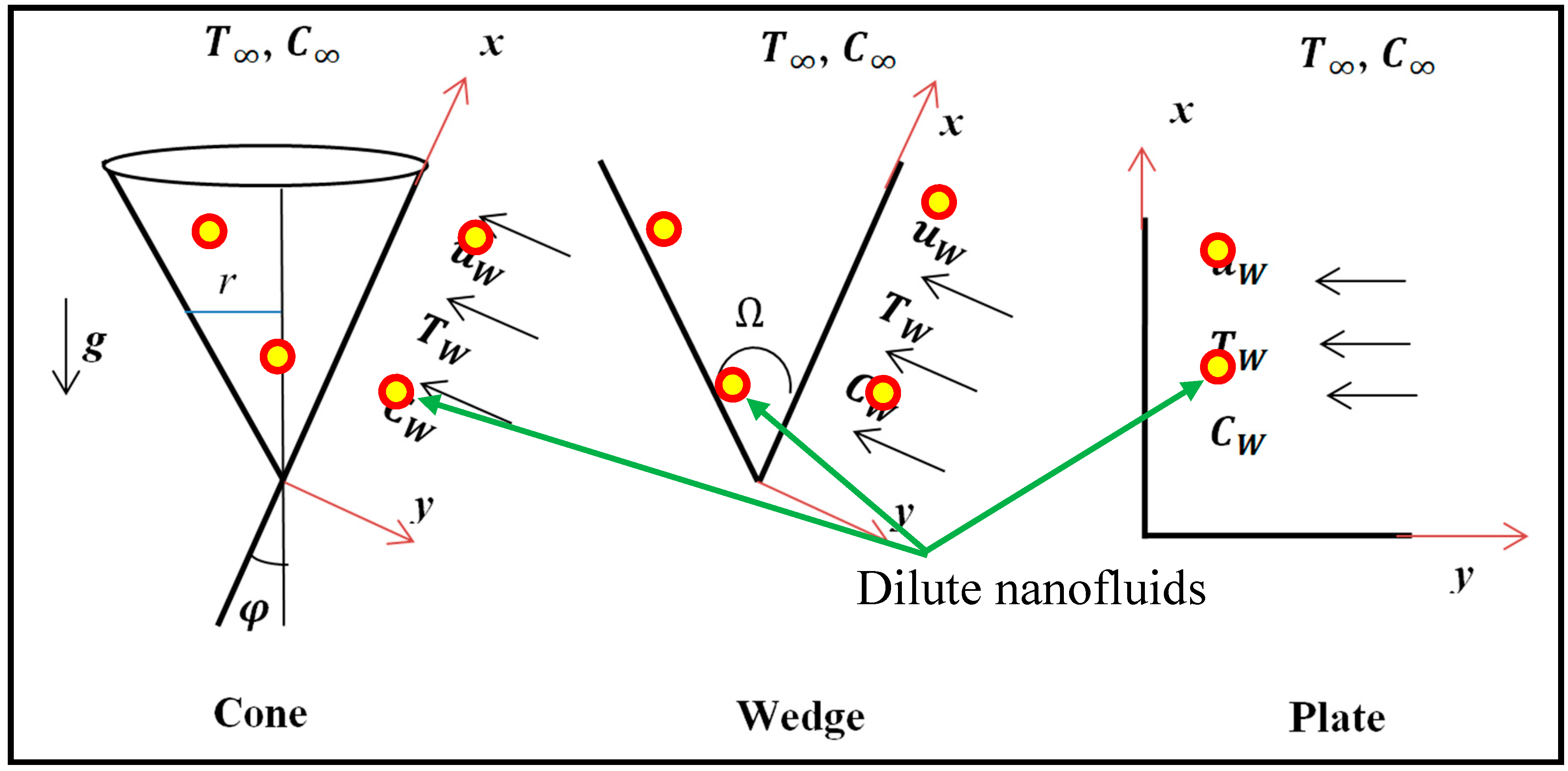
Consider the steady, incompressible and laminar flow of a non-Newtonian power-law nanofluid over three different geometrical surfaces, i.e., vertical cone, wedge and plate. Convective conditions are imposed at the boundary surface of the geometries. The effects of Brownian movement and thermophoresis are incorporated. The surface of the geometries is assumed to be stretched with velocity u W = x ν l 2 and the surfaces are assumed to be transpiration (suction/injection) velocity v W . The temperature and concentration near the surface are prescribed as T w = T + a x r 1 and C w = C + b x r 2 , where r 1 and r 2 are the wall temperature and nanoparticle concentration parameters. r 1 = 0 implies constant temperature at the wall (iso-thermal) and r 2 = 0 corresponds to constant wall nanoparticle concentration (iso-solutal). The suspension of nanoparticles is dilute and stable with no chemical reaction and negligible radiative heat transfer. The physical models for the three geometries are shown in Figure 1. T and C are ambient temperature and nanoparticle concentration respectively. The two dimensional co-ordinate axes are orientated such that the x -axis coincides with the wall (boundary) of each geometry which is prescribed convective condition. The y -axis is orthogonal to the wall as shown in Figure 1. φ is the semi-vertex cone angle, r is the radius of the cone and Ω is the vertex angle of the wedge. Dilute nanofluids are considered with spherical, homogenously distributed nano-particles.
The model shows three geometries (cone, wedge and plate) based on the following conditions:
(a)
m = 1 and φ 0 : cone
(b)
m = 0 and φ 0 : wedge
(c)
m = 0 and φ = 0 : plate
As per the quoted restraints, the general conservation equations which govern the flow over all three geometries can be expressed as:
x ( u r m ) + y ( v r m ) = 0  
u u x + v u y = n ν ( u y ) n 1 2 u y 2 + g ( ( 1 C ) ρ f β T ( T T ) β c ( ρ p ρ f ) ( C C ) ) cos α
u T x + v T y = α 2 T y 2 + τ [ D B C y T y + D T T ( T y ) 2 ]
u C x + v C y = D B 2 C y 2 + D T T 2 T y 2
The prescribed boundary conditions at the geometry wall and in the free stream:
u = u w ,   v = v w ,   k T y = h 1 ( T w T ) ,   D B C y + D T T T y   = 0 a t   y = 0 u 0 ,   T T ,   C C                    a s   y
where u and v are velocity component along x and y directions. u w = x ν l 2 . ρ f and ν = μ ρ represent nanofluid density and kinematic viscosity respectively ( μ is dynamic viscosity and ρ is fluid density), k is nanofluid thermal conductivity, T is temperature, n is power index, D B is Brownian diffusion coefficient, D T is thermophoretic diffusion coefficient, T is ambient temperature, C is ambient concentration and τ is nanoparticle to base fluid heat capacity ratio. Apparent viscosity for power-law model is μ e f f = μ ( u y ) n 1 . The condition D B C y + D T T T y   = 0 controls the concentration of nanoparticle at the surface (i.e., the influence of distribution of nanoparticle volume fraction at the boundary is described by this condition). The condition k T y = h 1 ( T w T ) indicates the convective condition at the surface of the geometries.
Introducing the following transformations
u = x ν l 2 f ( η ) ,   v = ν ( m + 1 ) l f ( η ) ,   η = y l , ϕ ( η ) = C C C w C   and   θ ( η ) = T T T w T
Equations (2)–(4) thereby reduce to the following non-dimensional form (Equation (1) is automatically satisfied):
n ( 2 f η 2 ) n 1 3 f η 3 ( f η ) 2 + ( 1 + m ) f 2 f η 2 + ( G r θ + G c ϕ ) Cos α = 0
1 Pr 2 θ η 2 + ( m + 1 ) f θ η r 1 f η θ + N b θ η ϕ η + N t ( θ η ) 2 = 0
1 S c 2 ϕ η 2 + ( m + 1 ) f ϕ η r 2 ϕ f η + N t N b 2 θ η 2 = 0
The wall and free stream boundary conditions (5) reduced to:
η = 0 :   f η = 1 ,   f = S ,   θ η = γ ( θ 1 ) ,   ϕ η + N t N b θ η = 0 , η :   f η 0 ,   θ 0 ,   ϕ 0
Parameters appear in Equations (7)–(9): Pr = α μ C p is Prandtl number, N b = τ D B ( C w C ) v and N t = τ D T ( T w T ) v T denotes Brownian motion parameters and thermophoresis parameter, S c = ν D m is Schmidt number, γ = l h 1 k is temperature Biot number, G r = l 2 g β T ( T W T ) v u w and G c = l 2 g β C ( C W C ) v u w represent thermal Grashof numbers and solutal (nanoparticle species buoyancy) Grashof numbers respectively. Several gradient functions are of interest in materials processing (coating) engineering design. These are the friction factor C f (dimensionless surface shear stress function), local Nusselt number N u (dimensionless wall heat transfer gradient) and local Sherwood number S h (dimensionless nanoparticle wall mass transfer gradient) and these take the following definitions, respectively:
C f = C f * ρ U w 2 = ( f ( 0 ) ) n , N u = x q w k ( T w T ) = θ ( 0 )   and   S h = x J w D B ( C w C ) = ϕ ( 0 )

3. Solution Using Homotopy Analysis Method

Homotopy Analysis Method (HAM) has been used to solve the model defined by Equations (7)–(9) subject to the boundary conditions (10). HAM is a semi-analytical method developed by Liao [44] and has been implemented to solve many fluid dynamics, applied mathematics and multi-physical mechanics problems. This method does not rely upon any physical small/large parameter and hence provide convenient way to guarantee the series solution by using a special parameter known as convergence control parameter. Hashim et al. [45] obtained series solutions to systems of first and second order partial differential equations (PDEs) by applying HAM. Recently, Sheikholeslami et al. [46] used HAM to analyze the melting effect in nanofluid flow. Mabood et al. [47] implemented HAM to evaluate the MHD flow over exponentially stretching sheet with radiation effect. Sarvanthi and Gorla [48] scrutinized the influence of heat sink or source on chemically-reacting Maxwell elastic-viscous nanofluid over an exponential stretching surface with convective boundary conditions. Hayat et al. [49] examined the non-Fourier thermal convection of carbon nanotube fluids over a curved stretching surface. Other applications of HAM in biological fluid dynamics and nanoscale transport include [50,51,52]. To extract the solutions of Equations (7)–(9) subject to the boundary conditions (10) using HAM, we have considered initial guesses f 0 , θ 0 and ϕ 0 of f , θ and ϕ in the following form:
f 0 = S + 1 e η
θ 0 = γ γ + 1 e η
ϕ 0 = N t N b γ γ + 1 e η
The linear operators are selected as follows:
1 ( f ) = f f
2 ( θ ) = θ θ
3 ( ϕ ) = ϕ ϕ
with the following properties:
1 ( c 1 + c 2 e η + c 3 e η ) = 0
2 ( c 4 e η + c 5 e η ) = 0
3 ( c 6 e η + c 7 e η ) = 0
where c i ( 1 i 7 ) are the arbitrary constants. If p [ 0 , 1 ] is the embedding parameter, h 1 , h 2 and h 3 are convergence control parameters, then we construct the following zeroth-order deformation equations as:
( 1 p ) 1 [ f ( η ; p ) f 0 ( η ) ] = p h 1 N 1 [ ( f ( η ; p ) , θ ( η ; p ) , ϕ ( η ; p ) , χ ( η ; p ) ) ]
( 1 p ) 2 [ θ ( η ; p ) θ 0 ( η ) ] = p h 2 N 2 [ ( f ( η ; p ) , θ ( η ; p ) , ϕ ( η ; p ) , χ ( η ; p ) ) ]
( 1 p ) 3 [ ϕ ( η ; p ) ϕ 0 ( η ) ] = p h 3 N 3 [ ( f ( η ; p ) , θ ( η ; p ) , ϕ ( η ; p ) , χ ( η ; p ) ) ]
The appropriate forms of the boundary conditions are now:
f ( 0 , p ) = 0 ,   f ( 0 , p ) = S   and   f ( , p ) 0
θ ( 0 , p ) = γ ( θ ( 0 , p ) 1 ) ,   θ ( , p ) 0
N t θ ( 0 , p ) + N b ϕ ( 0 , p ) = 0 ,   ϕ ( , p ) 0
The nonlinear operators N 1 ,   N 2 and N 3 are defined based on Equations (7)–(9) as below:
N 1 ( f ( η ; p ) , θ ( η ; p ) , ϕ ( η ; p ) ) = n 3 f ( η ; p ) η 3 ( 2 f ( η ; p ) η 2 ) ε + ( m + 1 ) f ( η ; p ) 2 f ( η ; p ) η 2               ( f ( η ; p ) η ) 2 + ( G r θ ( η ; p ) + G c ϕ ( η ; p ) ) Cos α
N 2 ( f ( η ; p ) , θ ( η ; p ) , ϕ ( η ; p ) ) = 1 Pr 2 θ ( η ; p ) η 2 r 1 θ ( η ; p ) f ( η ; p ) η + ( m + 1 ) f ( η ; p ) θ ( η ; p ) η               + N b θ ( η ; p ) η ϕ ( η ; p ) η + N t ( θ ( η ; p ) η ) 2
N 3 ( f ( η ; p ) , θ ( η ; p ) , ϕ ( η ; p ) ) = 1 S c 2 ϕ ( η ; p ) η 2 + ( m + 1 ) f ( η ; p ) ϕ ( η ; p ) η               r 2 ϕ ( η ; p ) f ( η ; p ) η + N t N b 2 θ ( η ; p ) η 2
In Equation (17a), ε = n 1 . When p = 0 and p = 1 , we obtain:
f ( η ; 0 ) = f 0 ( η ) f ( η ; 1 ) = f ( η )
θ ( η ; 0 ) = θ 0 ( η ) θ ( η ; 1 ) = θ ( η )
ϕ ( η ; 0 ) = ϕ 0 ( η ) ϕ ( η ; 1 ) = ϕ ( η )
The mth-order deformation equation can be obtained by differentiating the zeroth order deformation Equation 15a,d m times and dividing by m! This leads to:
1 [ f m ( η ; p ) χ m f m 1 ( η ) ] = h 1 R m f ( η )
2 [ θ m ( η ; p ) χ m θ m 1 ( η ) ] = h 2 R m θ ( η )
3 [ ϕ m ( η ; p ) χ m ϕ m 1 ( η ) ] = h 3 R m ϕ ( η )
The associated mth order deformation boundary conditions are:
f m ( 0 ) = 0 ,   f m ( 0 ) = 0   and   f m ( ) = 0
θ m ( 0 ) = γ θ m ( 0 ) ,   θ m ( ) = 0
N t θ m ( 0 ) + N b ϕ m ( 0 ) = 0 ,   ϕ m ( ) = 0
Where   χ m = { 0 ,   m 1 1 ,   m > 1   and R m f ( η ) = n H ε , i i = 0 m 1 f m i f i + ( 1 + m ) i = 0 m 1 f m i f i + ( G r θ m 1 + G c ϕ m 1 ) Cos α
Here:
H ε , i = 1 k ! { i p i ( 3 f p 3 [ 3 f p 3 ] ε ) } p = 0
R m θ ( η ) = 1 Pr θ m 1 + i = 0 m ( ( m + 1 ) f m 1 i θ i r 1 f m 1 i θ i + N b θ m 1 i ϕ i + N t θ m 1 i θ i )
R m θ ( η ) = 1 S c ϕ m 1 + i = 0 m ( ( m + 1 ) f m 1 i ϕ i r 2 f m 1 i ϕ i ) + N t N b θ m 1
Therefore, as p increases from 0 to 1 then f ( η ; p ) , θ ( η ; p ) and ϕ ( η ; p ) vary from initial approximations to the exact solutions of the original nonlinear differential equations.
Now, expanding f ( η ; p ) , θ ( η ; p ) and ϕ ( η ; p ) in Taylor series w.r.to p; we have
f ( η ; p ) = f 0 ( η ) + m = 1 f m ( η ) p m
θ ( η ; p ) = θ 0 ( η ) + m = 1 θ m ( η ) p m
ϕ ( η ; p ) = ϕ 0 ( η ) + m = 1 ϕ m ( η ) p m
where
f m ( η ) = 1 m ! m f ( η ; p ) p m | p = 0
θ m ( η ) = 1 m ! m θ ( η ; p ) p m | p = 0
ϕ m ( η ) = 1 m ! m ϕ ( η ; p ) p m | p = 0
If the initial approximations, auxiliary linear operators and non-zero auxiliary parameters are chosen in such a way that the series (22a)–(22c) are convergent at p = 1 then:
f ( η ) = f 0 ( η ) + m = 1 f m ( η )
θ ( η ) = θ 0 ( η ) + m = 1 θ m ( η )
ϕ ( η ) = ϕ 0 ( η ) + m = 1 ϕ m ( η )
where
f m ( η ) = f * m ( η ) + c 1 + c 2 e η + c 3 e η
θ m ( η ) = θ * m ( η ) + c 4 e η + c 5 e η
ϕ m ( η ) = ϕ * m ( η ) + c 6 e η + c 7 e η
f * m ( η ) , θ * m ( η ) and ϕ * m ( η ) are special solutions of the mth order deformation Equation (19a–c). The values of the constants c i ( 1 i 7 ) are:
c 1 = ( f m * ( 0 ) + f m * ( 0 ) ) ,   c 3 = f * m ( 0 ) ,   c 5 = θ * m ( 0 ) + γ θ * m ( 0 ) 1 γ , c 7 = ϕ m * ( 0 ) + N t N b ( θ * m ( 0 ) θ * m ( 0 ) + γ θ * m ( 0 ) 1 γ ) c 2 = c 4 = c 6 = 0
Substituting the values of c i ( 1 i 7 ) from (26) into (25a)–(25c) to have solution of mth order deformation Equation (19a–c), i.e., f * m ( η ) , θ * m ( η ) and ϕ * m ( η ) . Finally, the convergent series solution (24a)–(24c) is obtained using (25a)–(25c).

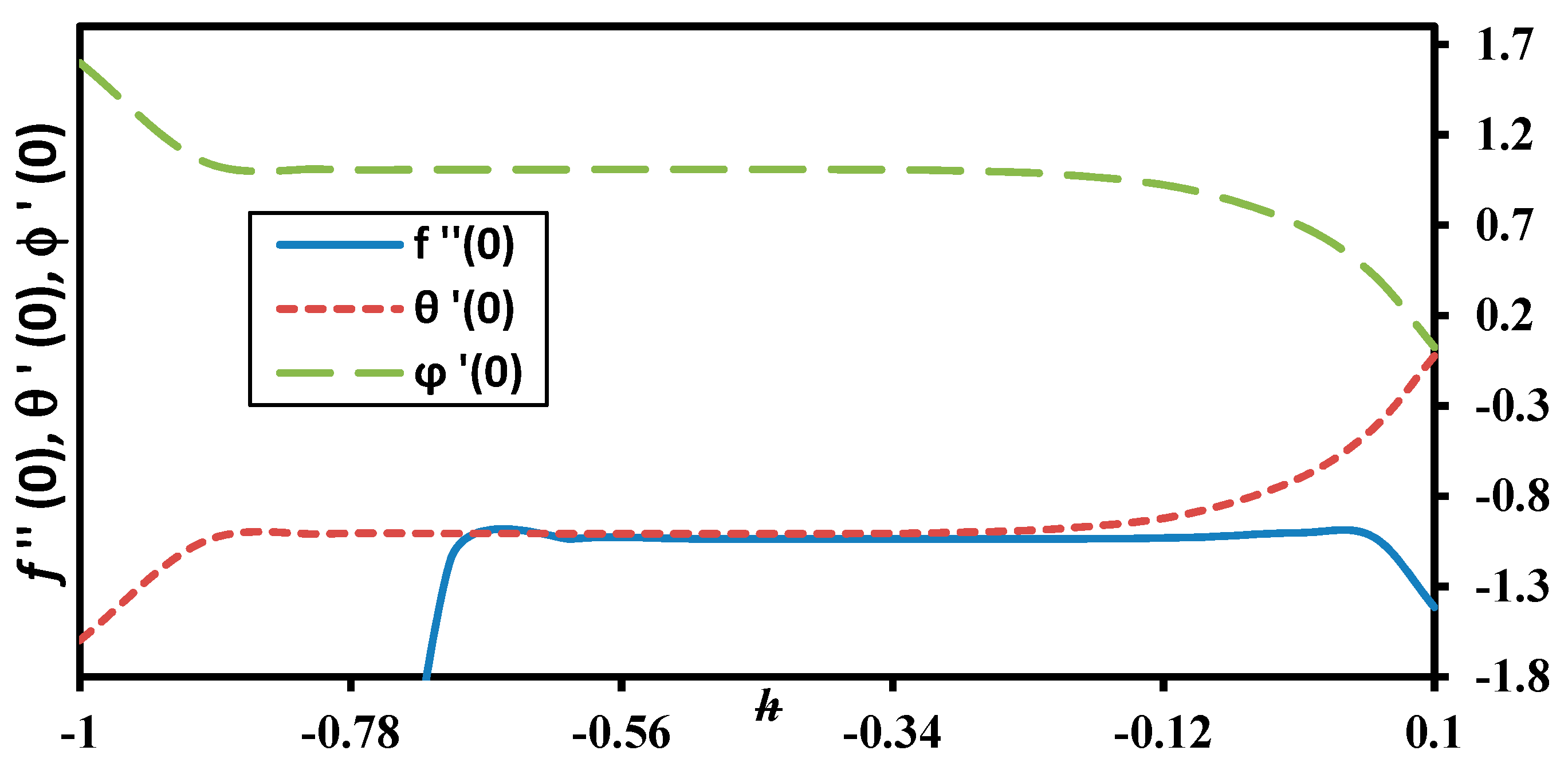
Convergence of Homotopy Series Solution

The homotopy solutions (21a)–(21c) for Equations (7)–(9) subject to the boundary conditions (10) is obtained using initial guesses f 0 , θ 0 and ϕ 0 given in Equation (12a–12c) and linear operators 1 ( f ) , 2 ( θ ) and 3 ( ϕ ) given in Equation (13a–13c) with the suitable values for the non-zero control parameters h 1 , h 2 and h 3 that have been obtained by plotting the h -curves shown in Figure 2. From Figure 2, it is seen that the valid regions of h 1 is (−0.1, −0.36) and of h 2 and h 3 is about (−0.1, −0.55). Here, h 1 = h 2 = h 3   = 0.35 is considered for the present study. Computations are performed using Mathematica 9 software with the thermophysical parameters: n = 3 ,   G r = G c = 0.5 , Pr = 1 ,   S = 0.1 ,   r 1 = r 2 = 1 ,   S c = 1.2 ,   N t = N b = 0.1 ,   γ = 2 .
The convergence of homotopy series solution is given Table 1 and concludes that 16th order of approximation is appropriate for computations since negligible variations are observed for higher orders of approximation. 16th order of approximation is taken for the computation throughout the study. The present study is compared with the existing results of Hassanien et al. [53] for the validation of the HAM computations as shown in Table 2. Computational time and error analysis with respect to different residual errors is explained in Table 3. Here, the obtained data elaborates that the computational time depends on the complexity of the geometries.
It is clear from Table 3 that computations require greater compilation times for the cone compared with the wedge and plate to achieve the same accuracy of order 10−7. With the same set of parameters, the order of approximation as well as the computational time for the plate is generally less. The computations have been performed in system processor: Intel(R) Core (TM) i5–5200U CPU@ 2.20 GHz and system type: 64-bit MS Windows 10 operating system. The symbolic software Mathematica has been used to compute the results.

4. Results and Discussion

The set of transformed coupled nonlinear ordinary differential Equations (7)–(9) subject to boundary condition (10) are solved very efficiently using HAM. To investigate the evolution in velocity, temperature and volume fraction profiles, we set values of the parameters, i.e., Prandtl number, Schmidt number, thermophoresis and Brownian motion parameter and suction/injection parameteras n = 3 ,   G r = G c = 0.5 ,   Pr = 2 ,   S = 0.1 ,   r 1 = r 2 = 1 ,   S c = 1.2 ,   γ = 2 .
The main focus of this article is to analyze the effect of the revised Buongiorno model on the convective flow of non-Newtonian power-law fluid over different geometries. With the aid of tables, the skin factor, Nusselt number and Sherwood number are properly explained for pertinent parameters. The half-cone angle φ is taken 45°.
Figure 3, Figure 4 and 
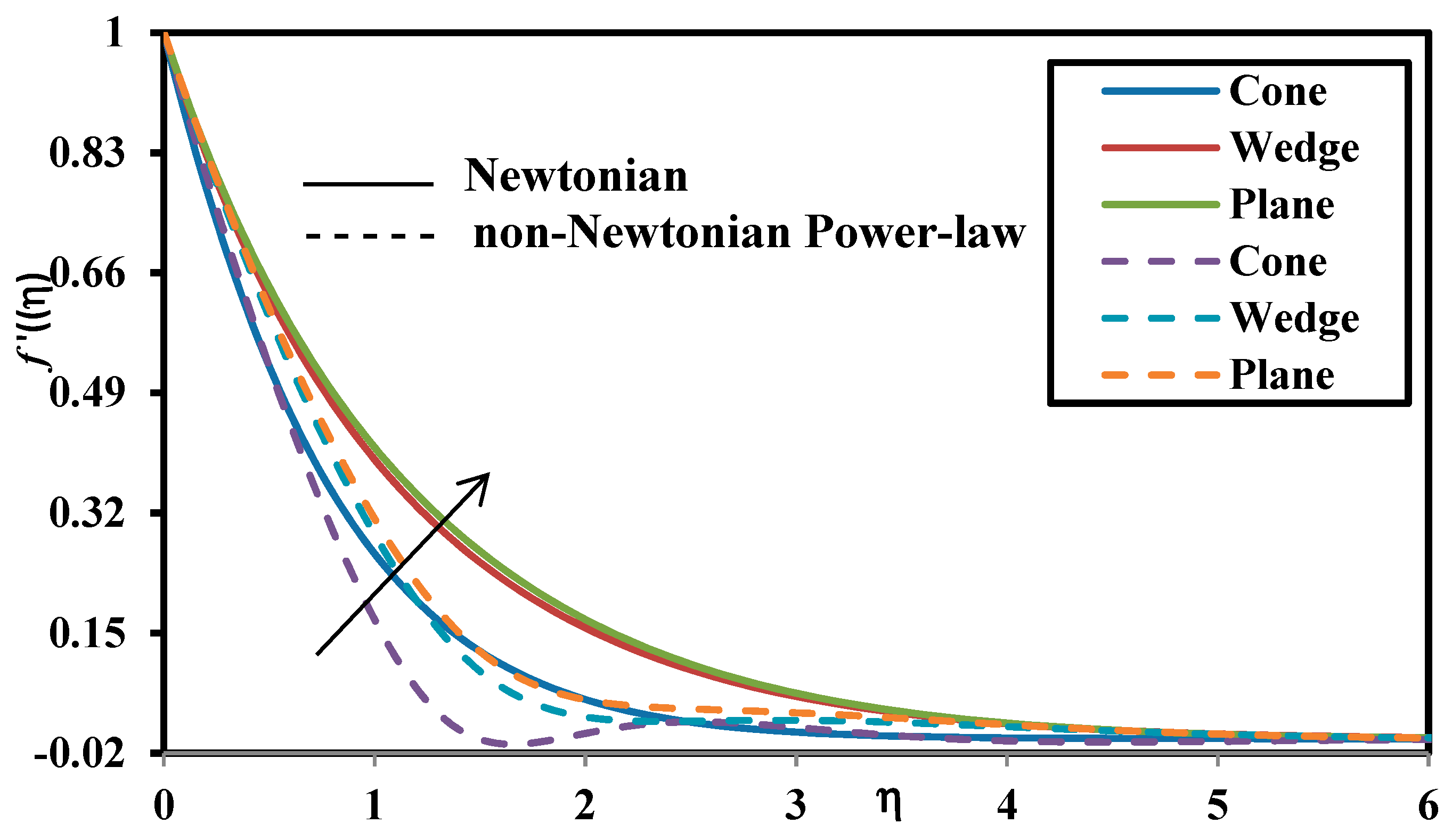
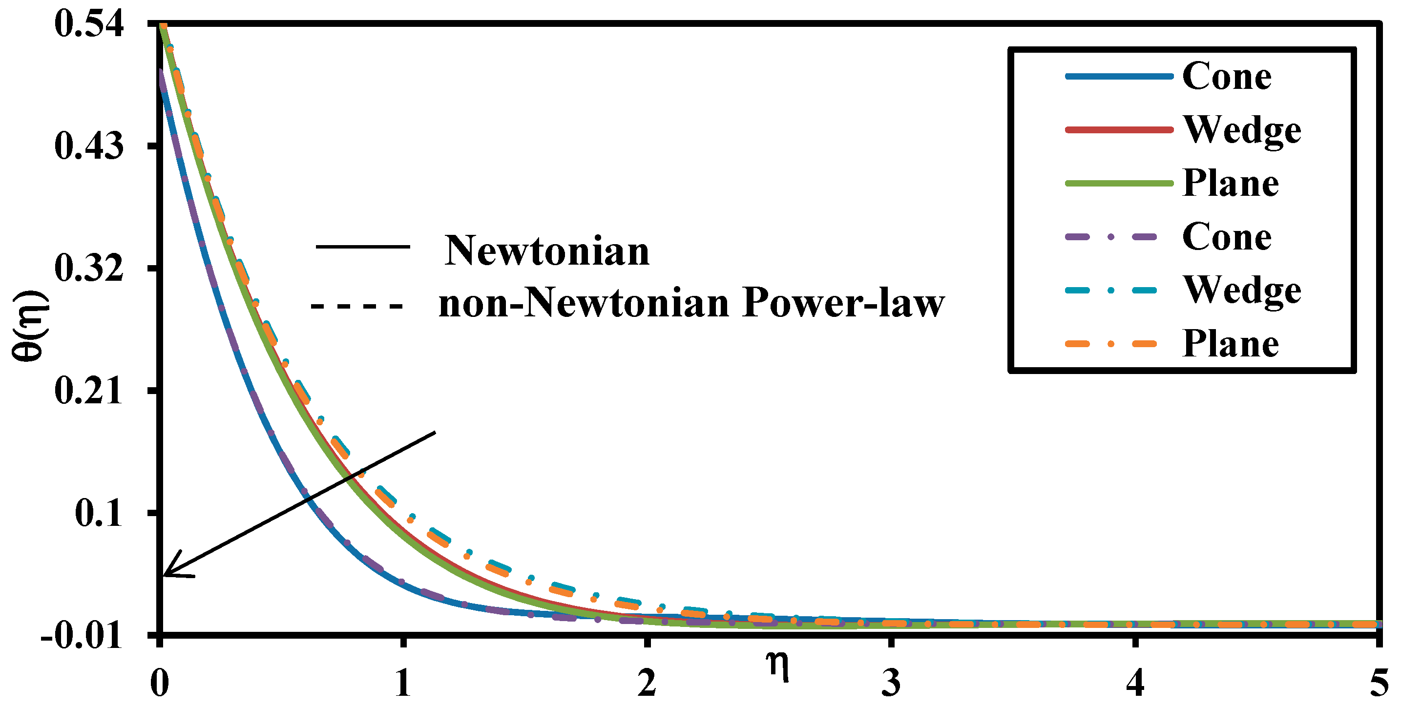
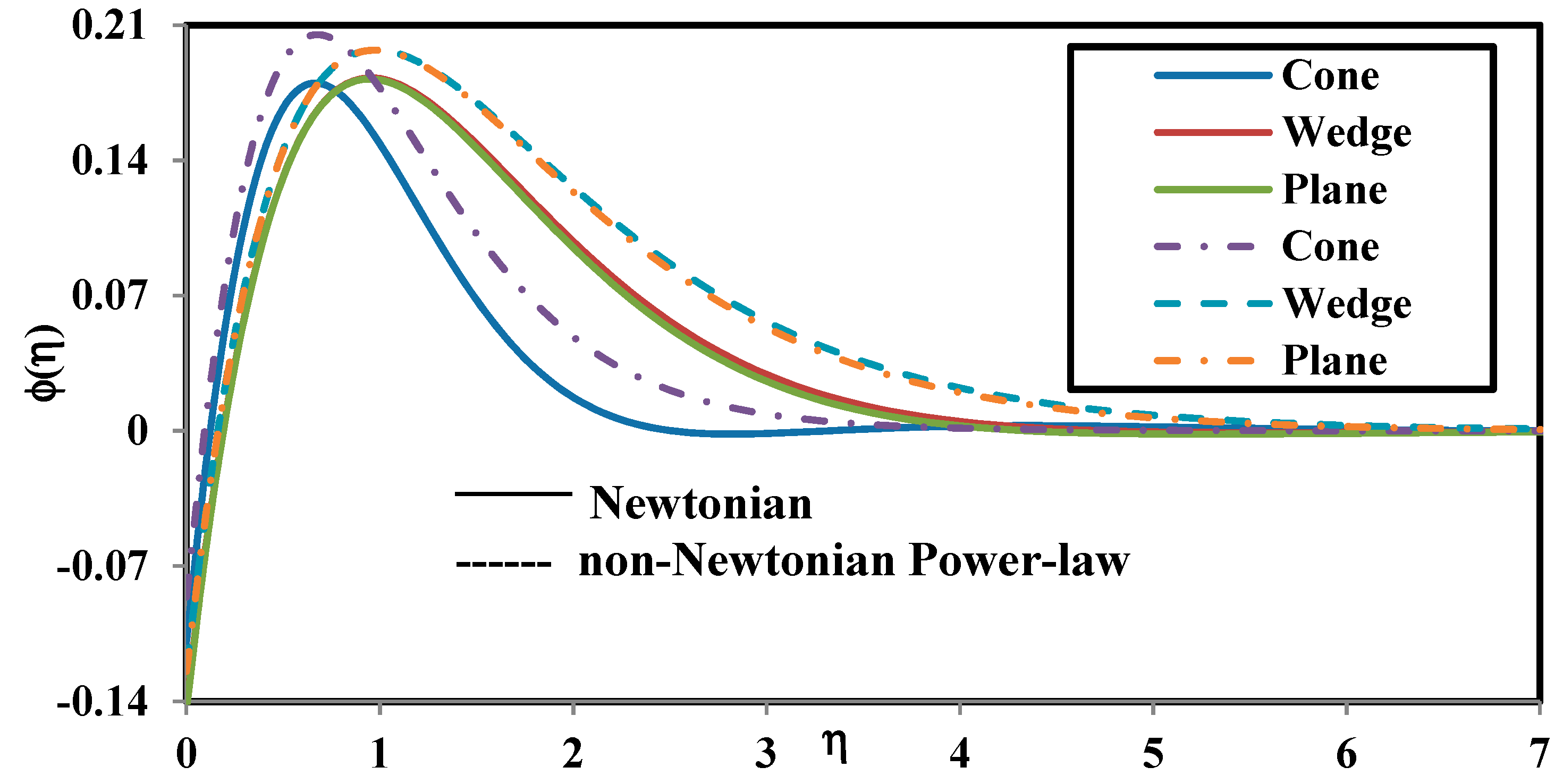
Figure 5 show the different response for Newtonian and non-Newtonian nanofluids via the velocity, temperature and nanoparticle concentration profiles for the cone, wedge and plate. It is clearly seen from Figure 3 that the velocity of both Newtonian and non-Newtonian fluid over the plate exceeds that computed for the wedge and plate. Additionally, the power-law nanofluid suppresses the velocity as compared to Newtonian nanofluid for all geometries, i.e., it thickens the momentum boundary layer for all three geometries. The temperature and nanoparticle profiles for Newtonian nanofluid shown in Figure 4 and Figure 5 are higher than for non-Newtonian fluid near to the surface of the geometries. The contrary behaviour is observed away from the surface of the plate and wedge. Since, the velocity for power-law flow reduces because of higher viscosity when compared with Newtonian fluid flow. Due to this reason, there is clogging of nanoparticle near the surface of the geometries which results in increasing the nanoparticle volume fraction.
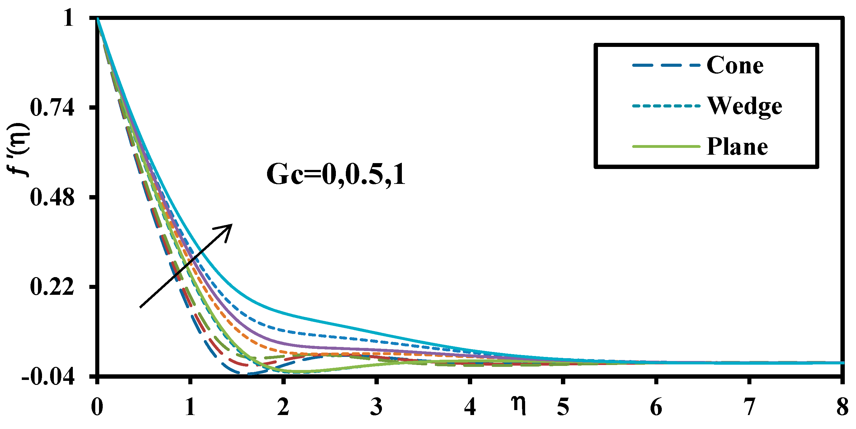
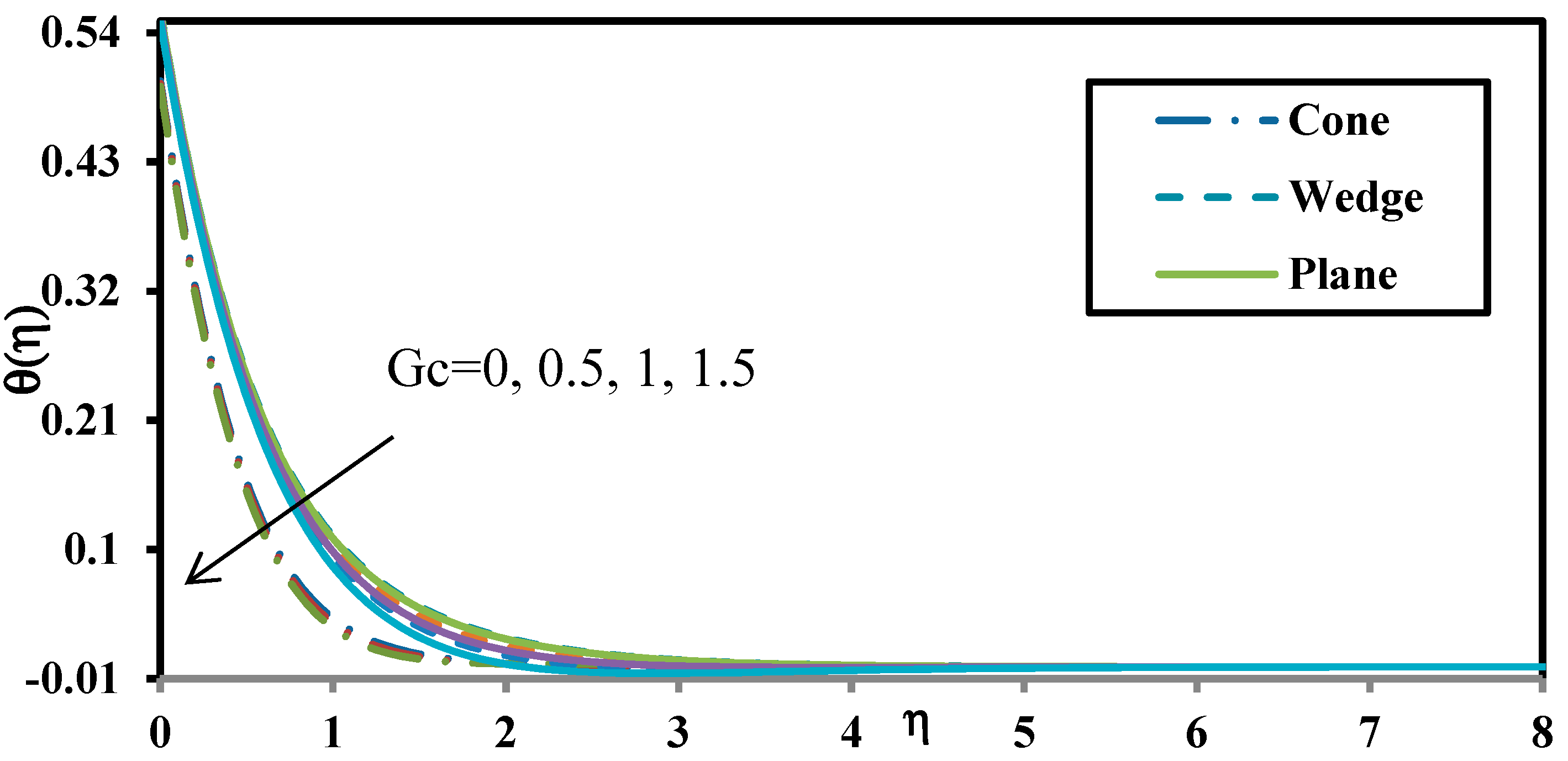
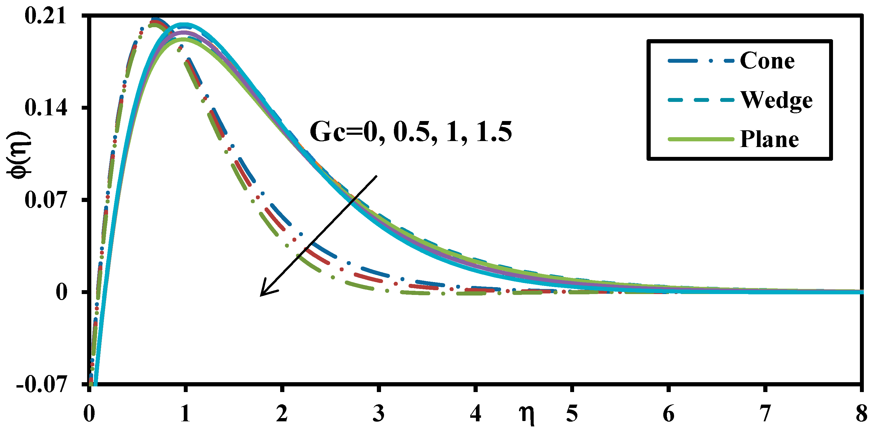
Figure 6, Figure 7 and 
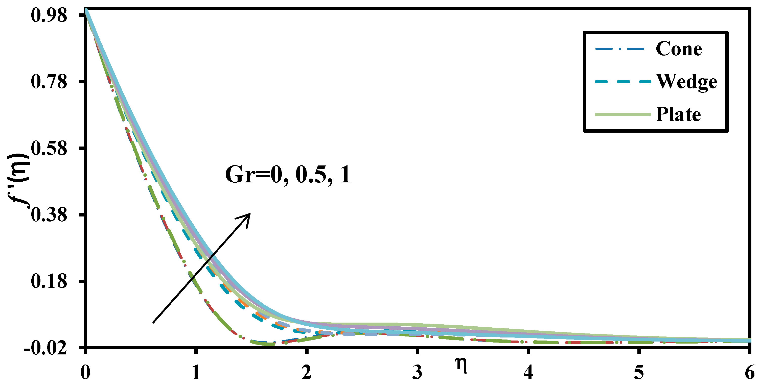
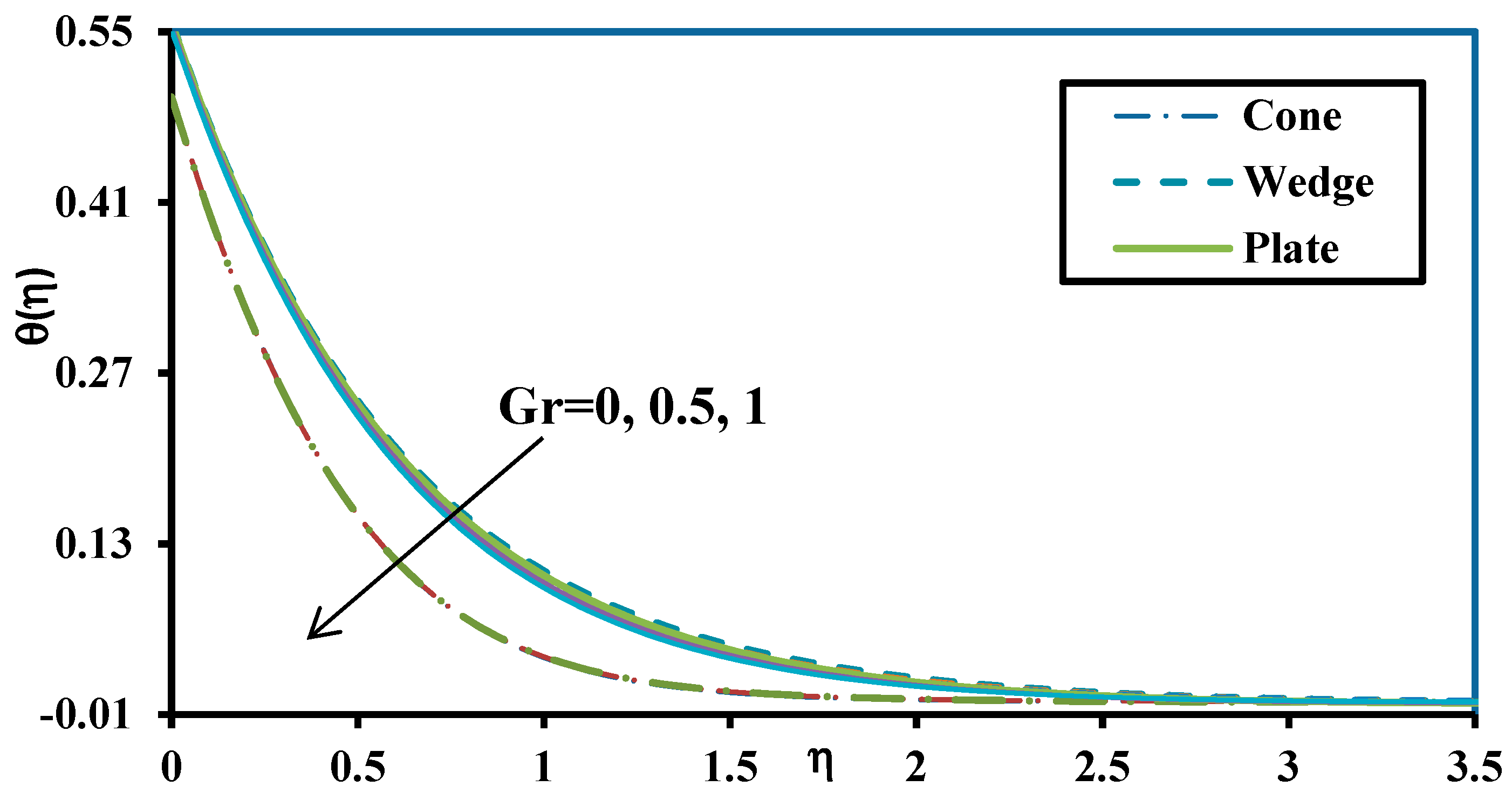
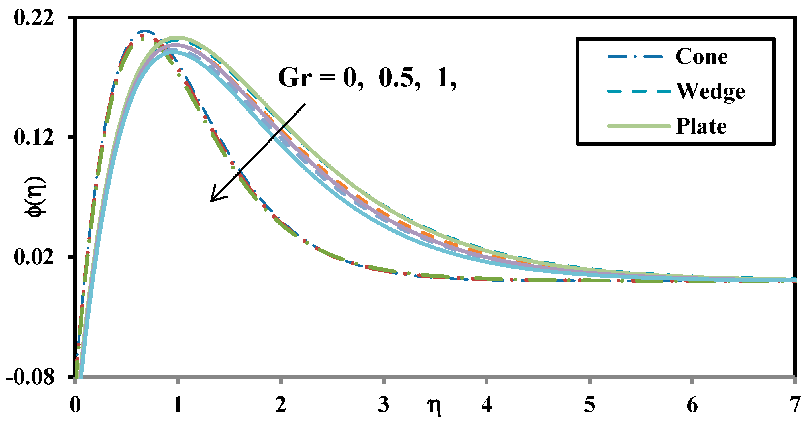
Figure 8 elucidate the effect of thermal Grashof number G r on the velocity, temperature and nano-particles volume fraction (concentration) for the cone, wedge and plate. A rise in value of Grashof number enhances the velocity whereas it depletes the temperature and nanoparticle volume fraction. Therefore, hydrodynamic boundary layer thickness is reduced whereas thermal and nanoparticle concentration boundary layer thicknesses are elevated with thermal buoyancy. Increasing values of Grashof number correspond to a decrease in viscosity of the nanofluids which assist in momentum diffusion and flow acceleration. This boosts the velocity magnitudes for all geometries. It is also evident that the temperature and nanoparticle volume fraction are substantially greater for the wedge geometry as compared to the plate and cone geometries.
Figure 9, Figure 10 and Figure 11 denote the variation of solute Grashof number G c on the velocity, temperature and nano-particles volume fraction for all geometries. Increasing values of solute Grashof number enlarge the velocity whereas they reduce the temperature and nanoparticle volume fraction magnitudes. The impact of nanoparticle solutal Grashof number induces a similar response to the effect of thermal Grashof number on all profiles and for geometries. Here G r = 0 and Gc = 0 indicates the absence of thermal and species buoyancy forces, respectively and corresponds to the forced convection scenario.
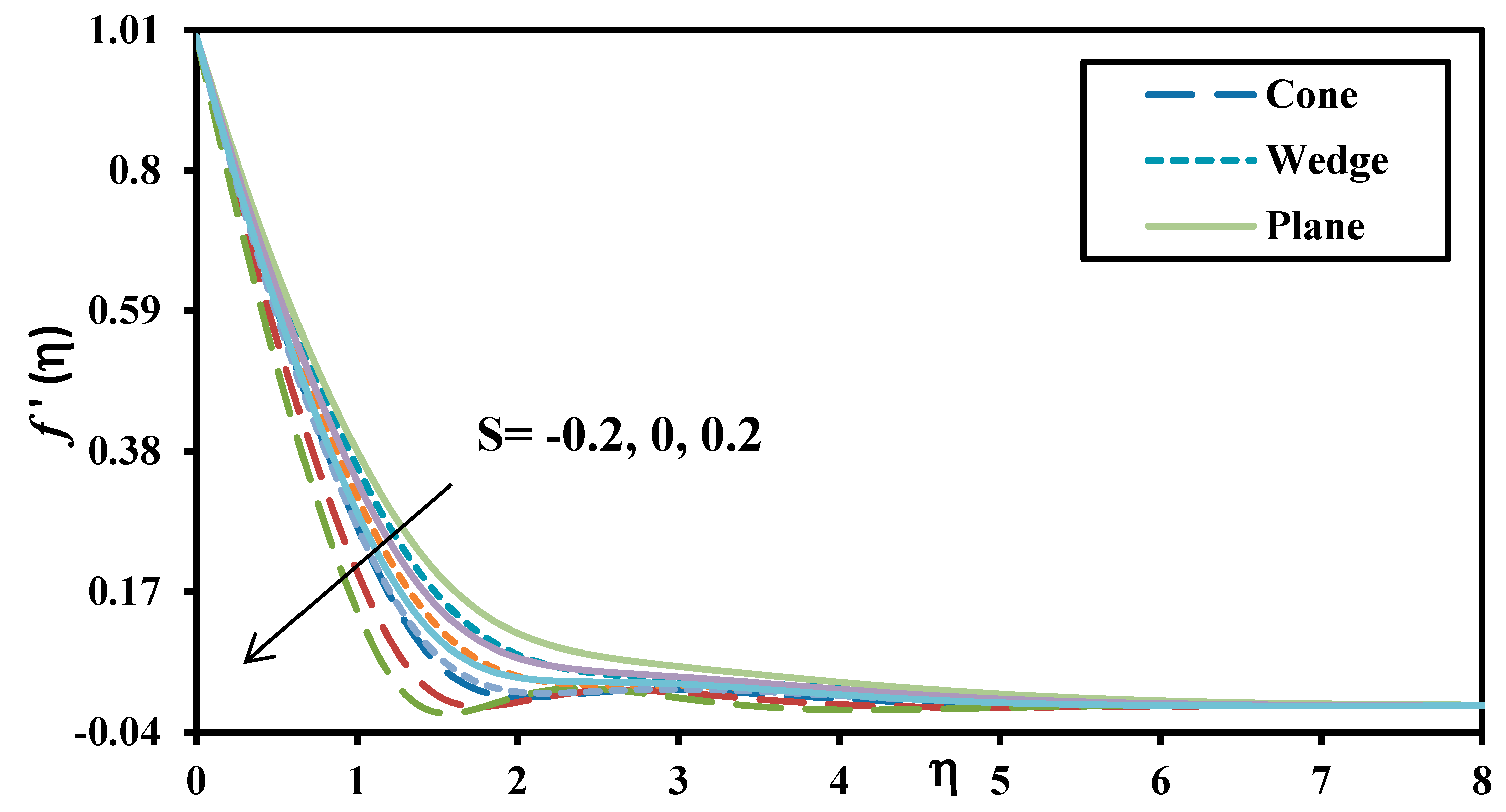
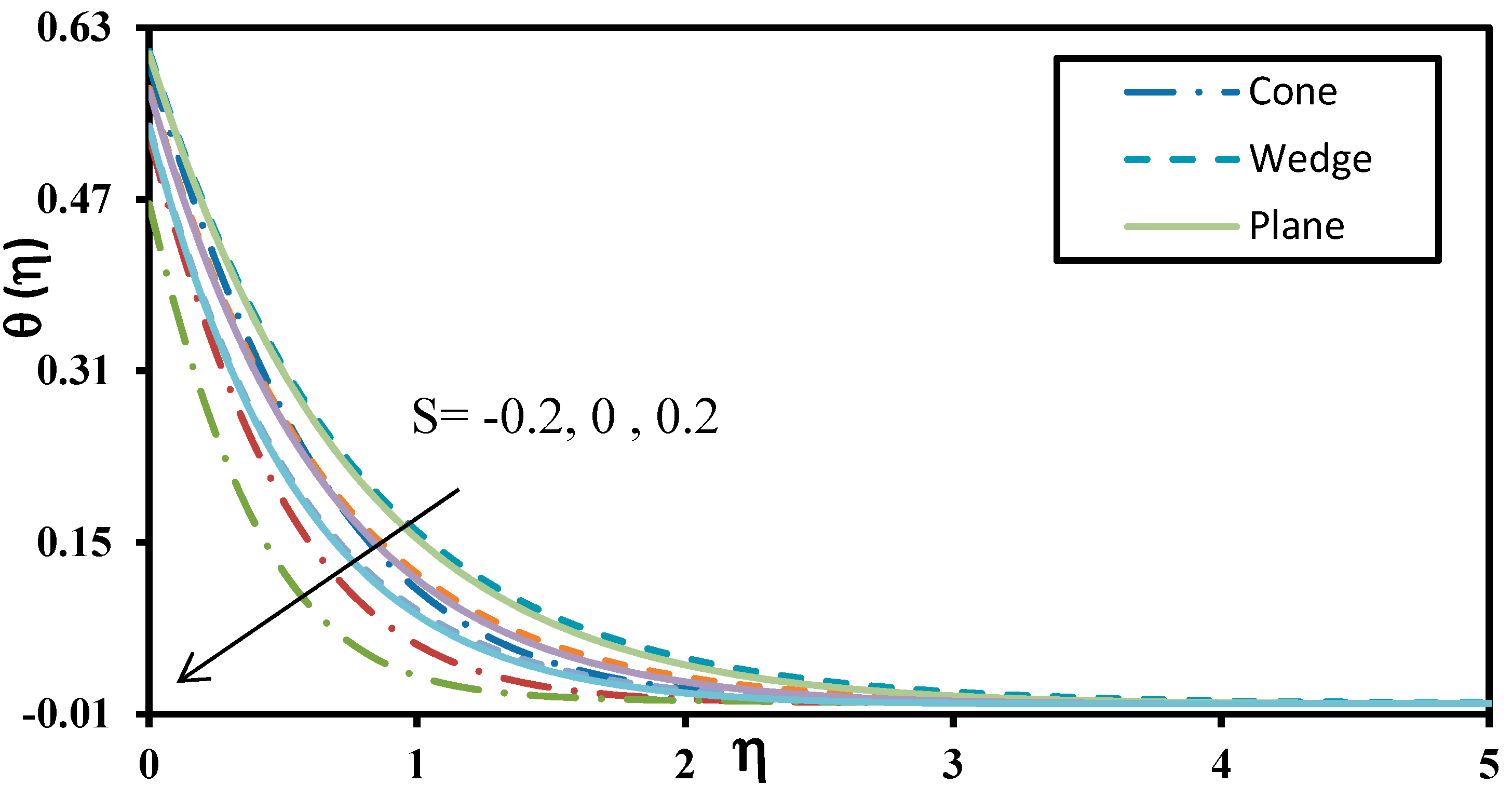
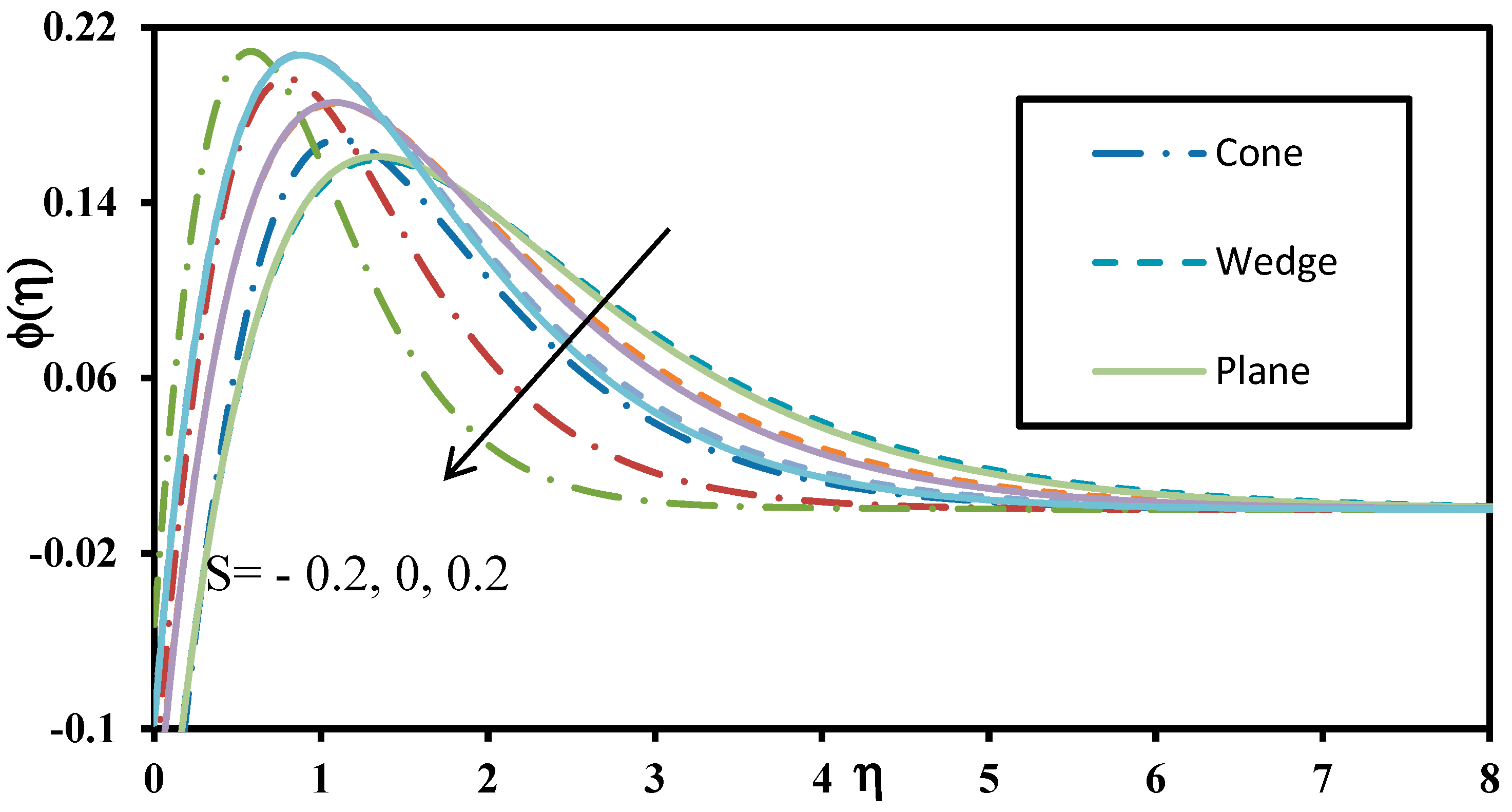
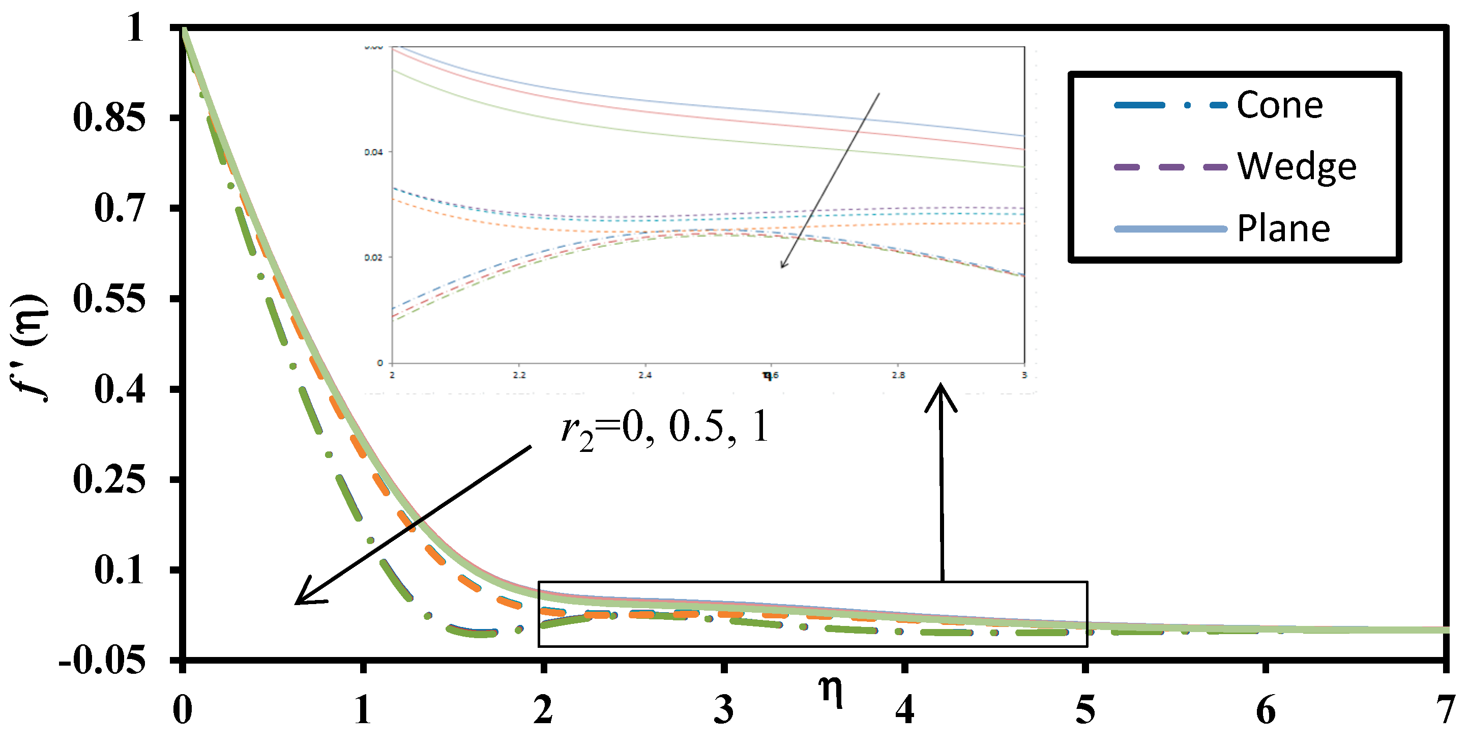
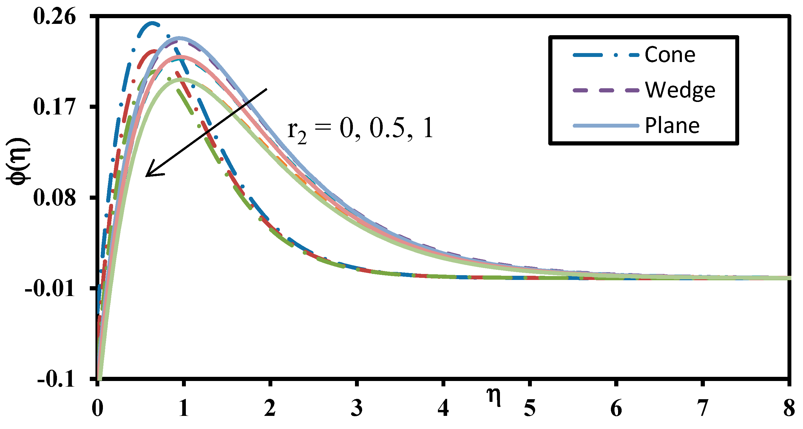
Figure 12, Figure 13 and Figure 14 shows the influence of wall suction on velocity, temperature and nanoparticle volume fraction for the cone, wedge and plate. Presence of suction lessens the velocity, temperature and concentration profiles. The suction effect induces stronger adherence of the nanofluid to the geometry wall and causes strong flow deceleration. This also inhibits thermal and nanoparticle diffusion so that thermal and nanoparticle boundary layer thicknesses are reduced. A greater modification in momentum boundary layer thickness is computed for the plate case whereas more significant alteration in thermal and concentration boundary layer thicknesses is computed for the wedge case.
Figure 15, Figure 16 and Figure 17 visualize the effect of wall temperature (isothermal and non-isothermal effect) on velocity, temperature and nanoparticle volume fraction. Due to increase in wall temperature, the boundary layer behaviour is influenced strongly. Velocity is lower and momentum boundary layer thickness is greater for the wedge when compared with the cone whereas momentum boundary layer thickness is lower than for the plate. Velocity, temperature and nanoparticle volume fraction profiles show higher values for constant wall temperature (isothermal case) compared with the non-isothermal case.
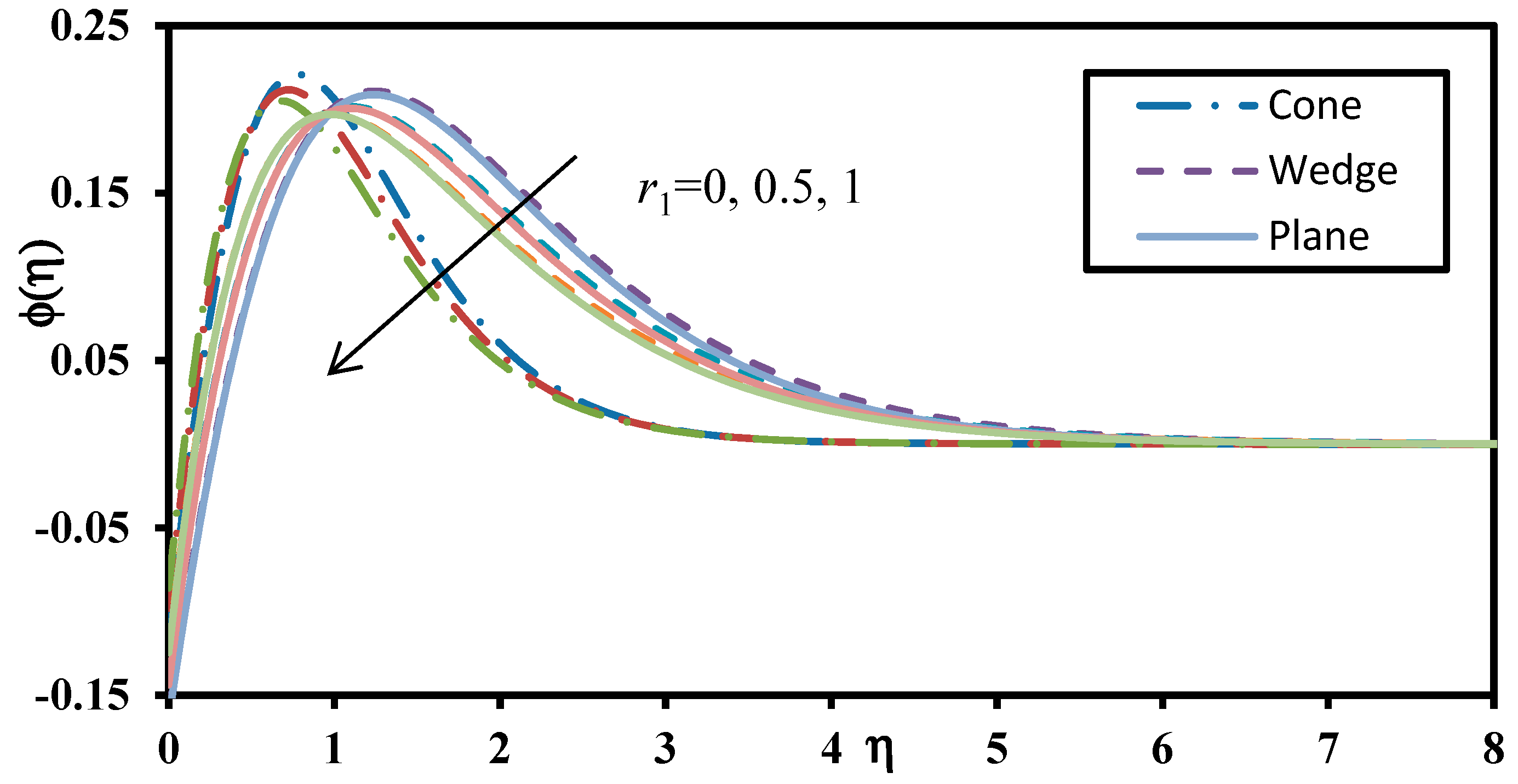
Figure 18, Figure 19 and Figure 20 show the effect of wall concentration (iso-solutal and non-iso-solutal effect) on velocity, temperature and nanoparticle volume fraction. Constant wall concentration generates higher values for all profiles. An increase in wall concentration results in a decrease in boundary layer thicknesses. The flow of nanofluid from a cone produces a lower velocity, temperature and nanoparticle volume fraction when compared to the plate and wedge scenarios.
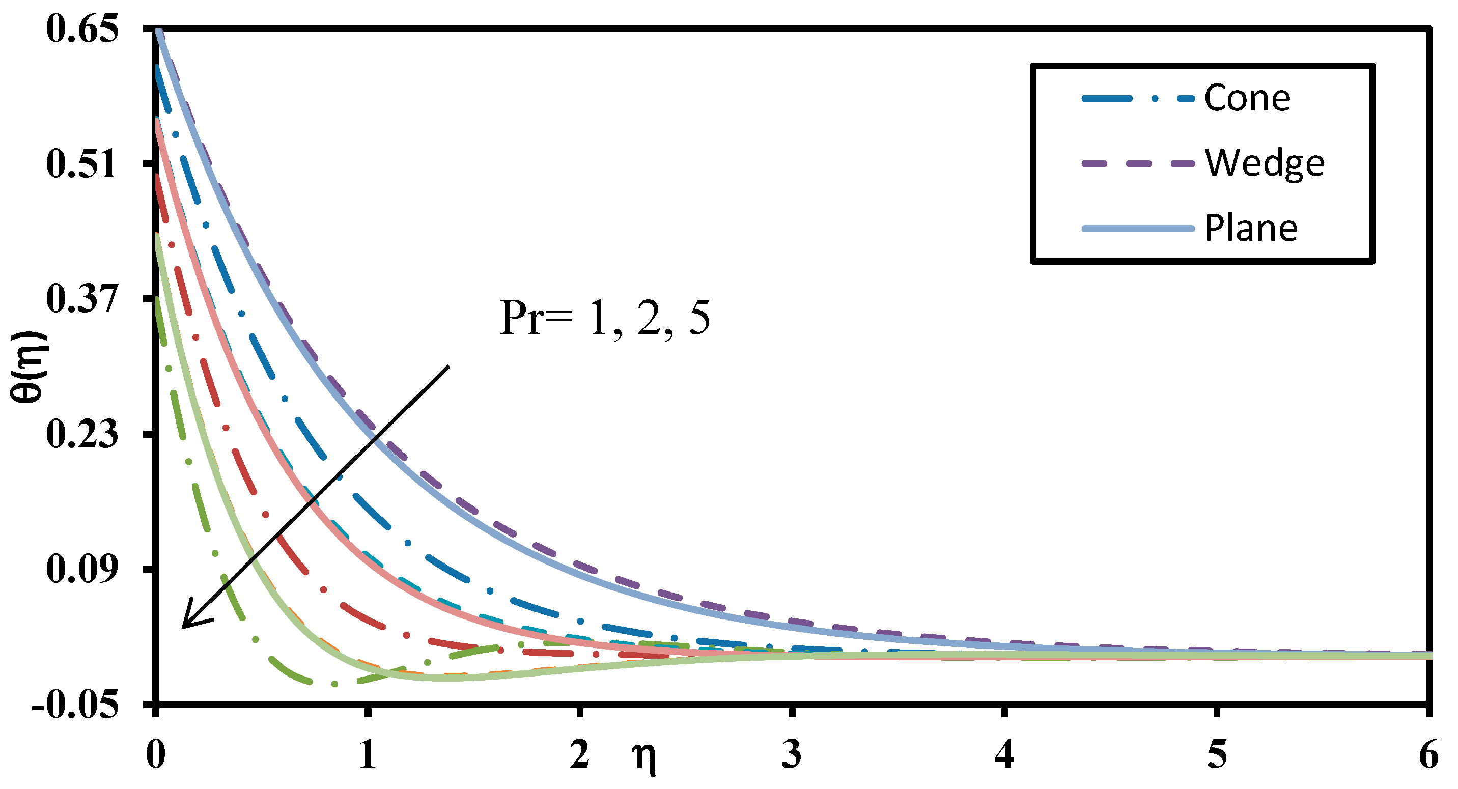
Figure 21 and Figure 22 depict the effect of Prandtl number on velocity, temperature and nanoparticle volume fraction for different geometries. Due to increase in Prandtl number, the momentum diffusivity increases which results in a decrease in velocity magnitudes (Figure 21). Figure 22 indicates that the heat transfer behaviour is highly dependent on the Prandtl number, a most important parameter in thermal convection. The temperature of the fluid decreases monotonically with the increasing Pr , i.e., thermal boundary layer thickness is suppressed. Clearly different responses are computed for the different geometries indicating that external geometry is a key player in controlling thermo-fluid characteristics in nanofluid boundary layer flows.
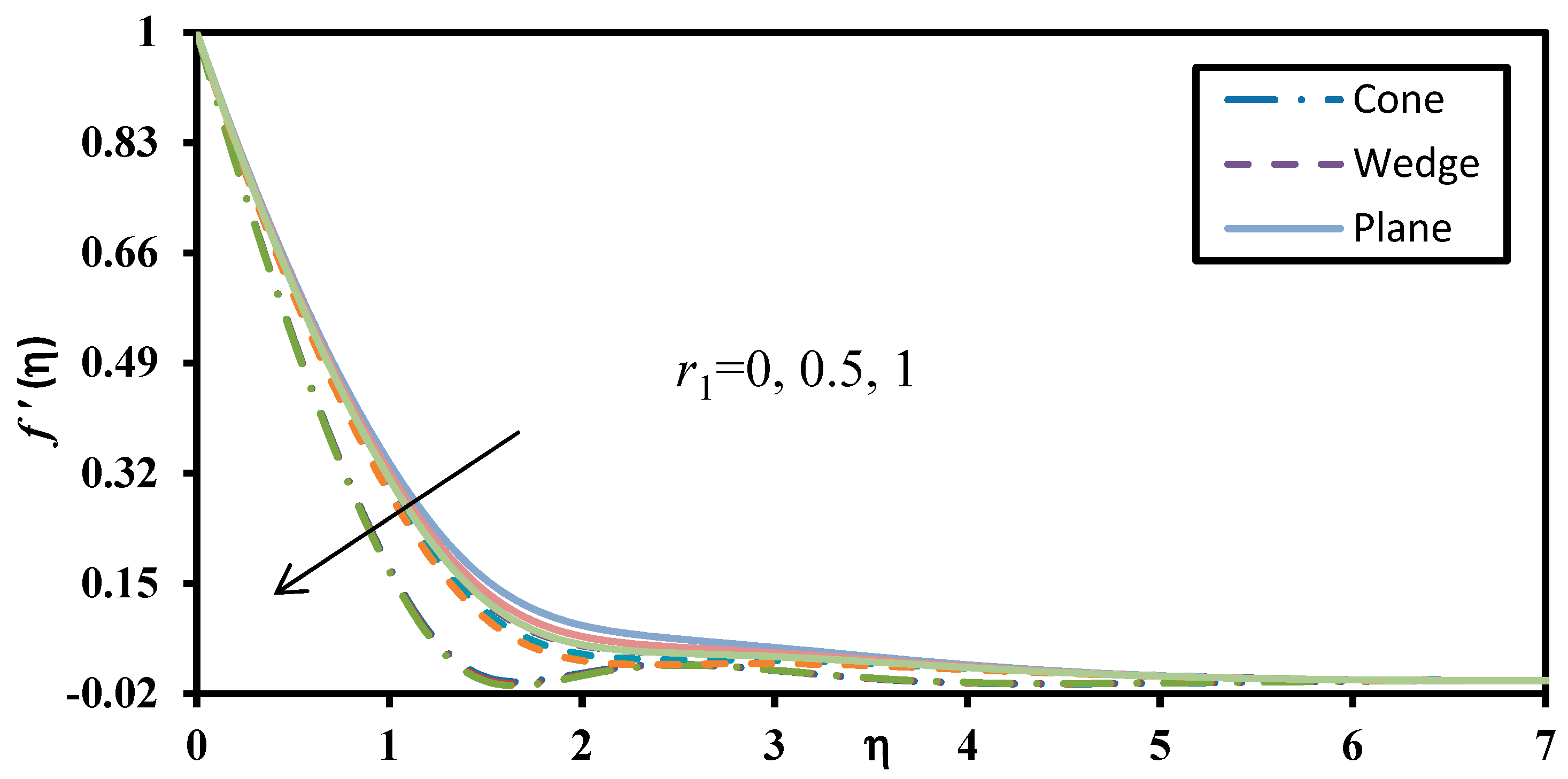
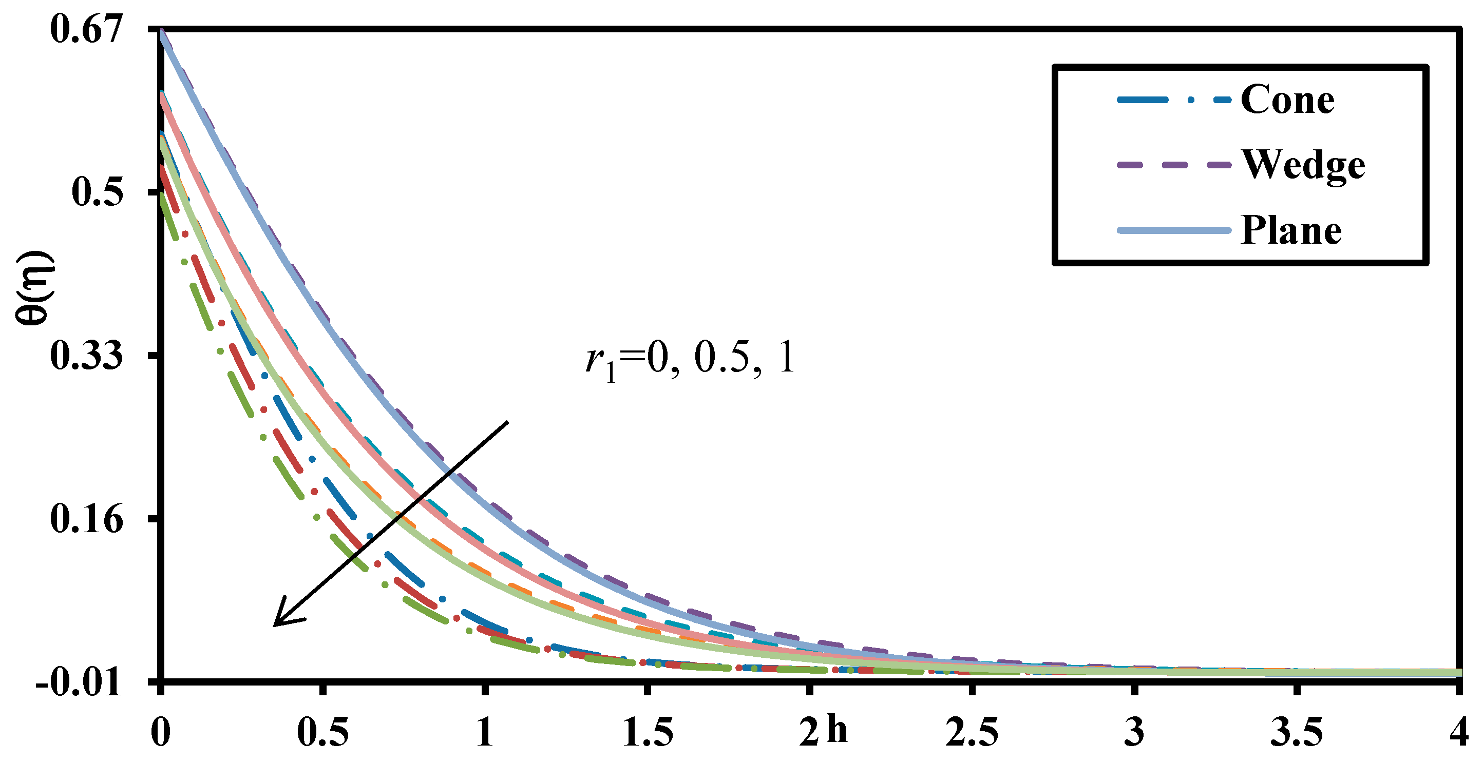
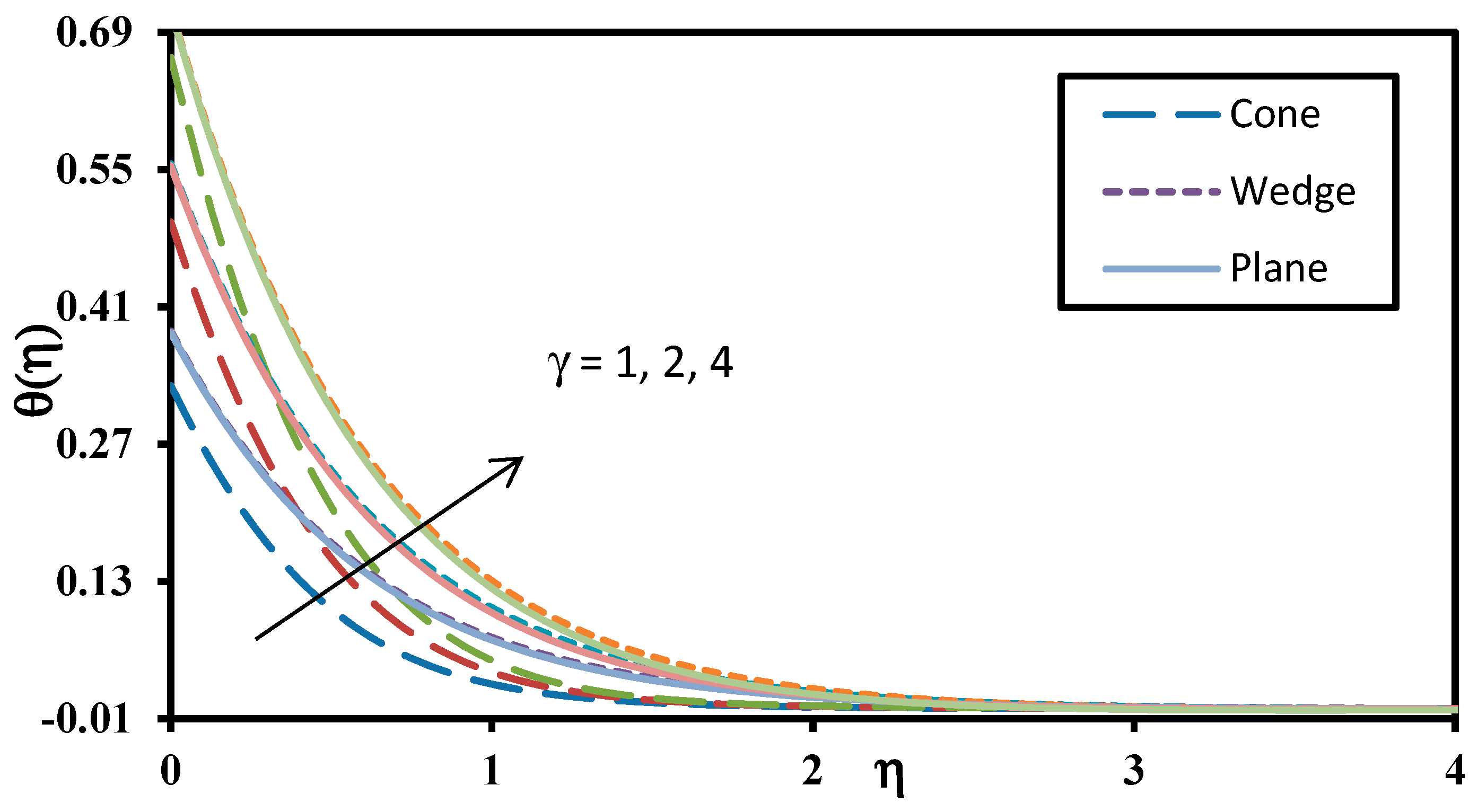
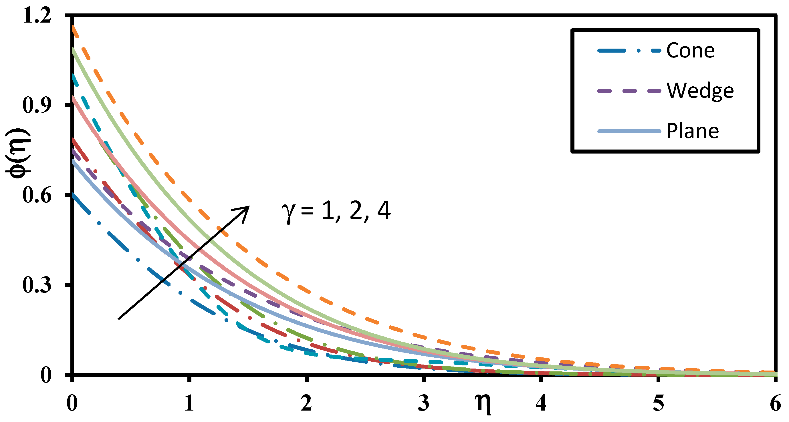
Figure 23, Figure 24 and Figure 25 displays the effect of Biot number (convective boundary condition parameter) on velocity, temperature and nanoparticle volume fraction for different geometries. Increase in thermal Biot number results in enhancement of the momentum, thermal and concentration boundary layer thickness. Additionally, it is observed from Figures that velocity of the non-Newtonian fluid flow for the plate is higher than the cone or wedge. The behaviour of Newtonian and non-Newtonian fluid flow over all geometries is similar.
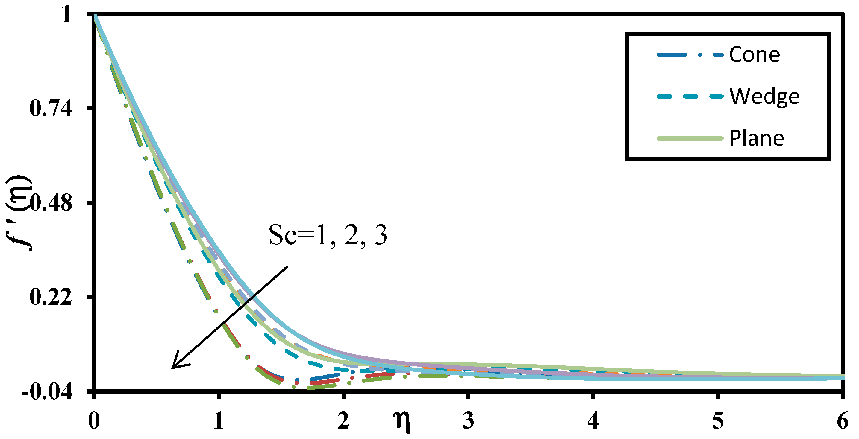
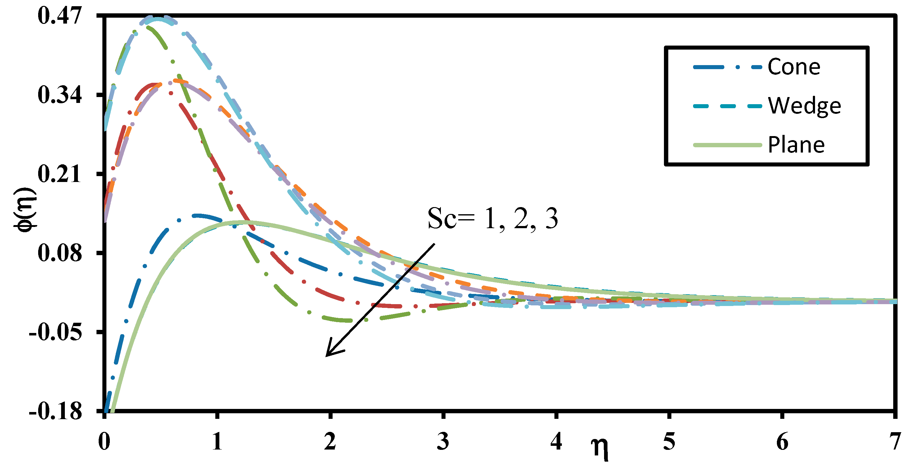
Figure 26 and Figure 27 illustrates the impact of Schmidt number on velocity distribution and nanoparticle volume fraction. Figure 27 demonstrates that the momentum boundary layer thickness lessens with increasing value of Schmidt number since the flow is strongly accelerated. Figure 27 shows that an increase in Schmidt number results in a decrease in nanoparticle concentration values. This reduction in nano-particles concentration is due to the change in Brownian diffusion coefficient. Enlarging Schmidt number corresponds to weaker Brownian diffusion coefficient and inhibited diffusion of nanoparticles through the boundary layer regime. This also results in depletion in nanoparticle concentration boundary layer thickness.
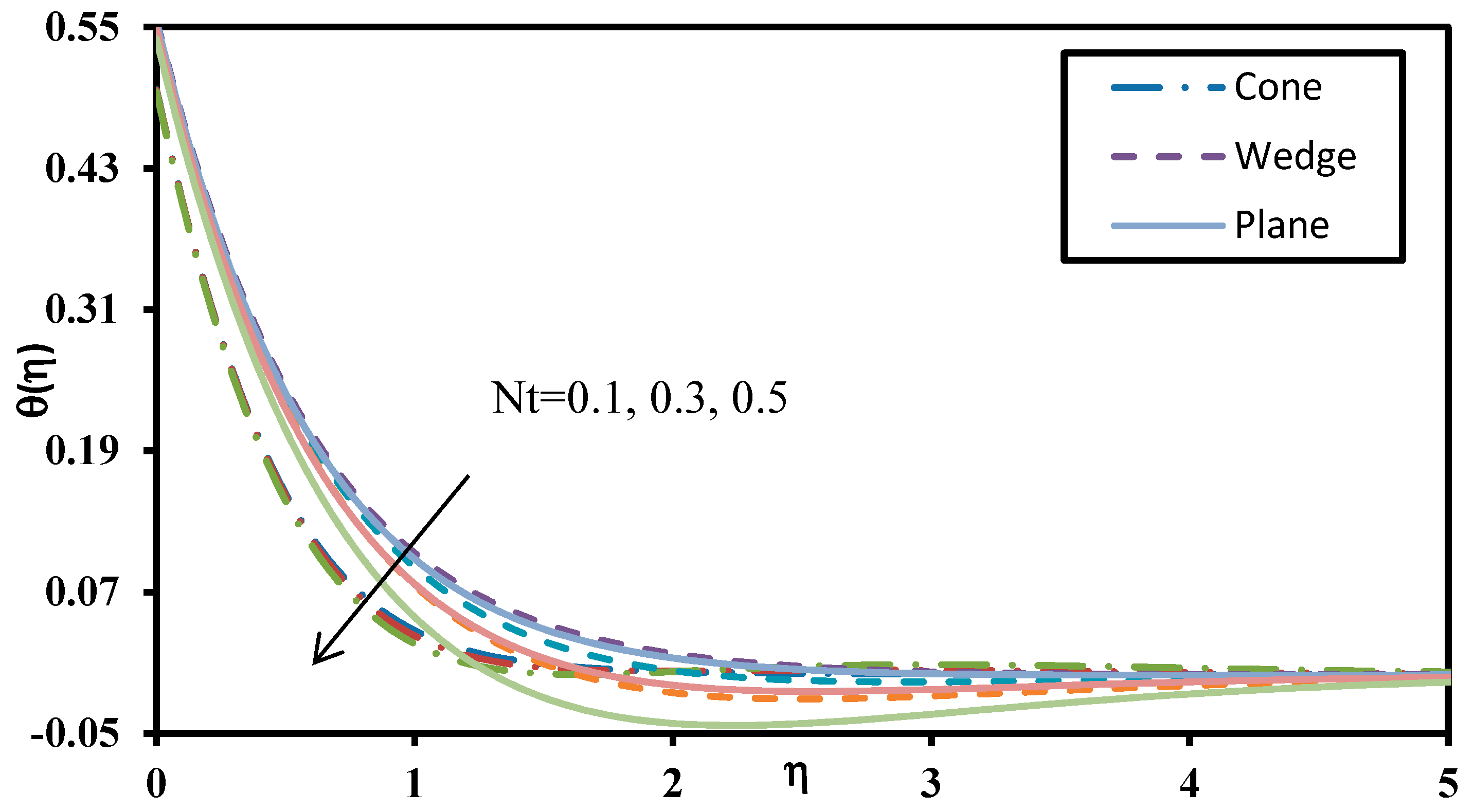
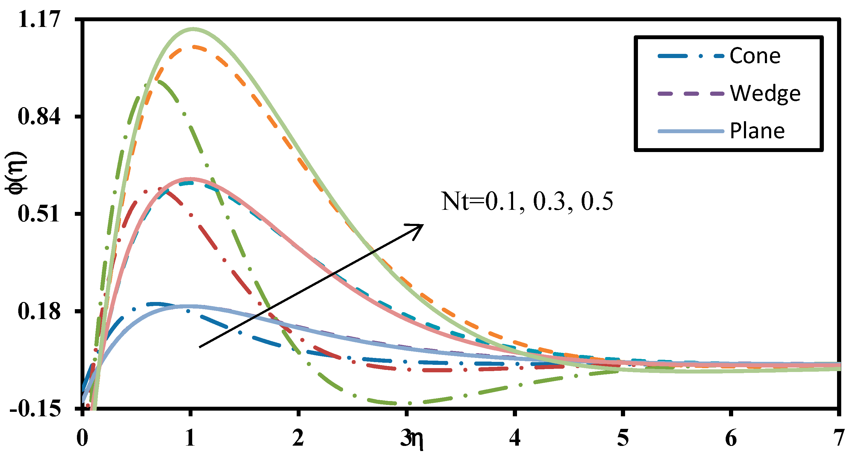
Figure 28 and Figure 29 depicts the effect of thermophoresis parameter on temperature and nanoparticle volume fraction respectively for different geometries. Higher thermophoresis implies greater migration of hot nanoparticles in the direction of a decreasing temperature gradient which encourages nanoparticle diffusion in the boundary layer. Thermophoretic forces exerted on the nanoparticles are in the opposite direction to the actual temperature gradient. This effectively results in a thickening in the nanoparticle concentration boundary layer thickness for all the geometries studied. Due to affect of convective boundary condition and modified Buongiorno model, the behaviour of temperature and nanoparticle volume fraction is different by varying N t . Temperature field is a decreasing function of thermophoresis parameter N t whereas nanoparticle volume fraction is an increasing function of N t (see Figure 29). Thermal boundary layer thickness is therefore decreased with stronger thermophoresis. Temperature and nanoparticle volume fraction (concentration) profiles for the wedge exceed those for the plate and cone geometries.
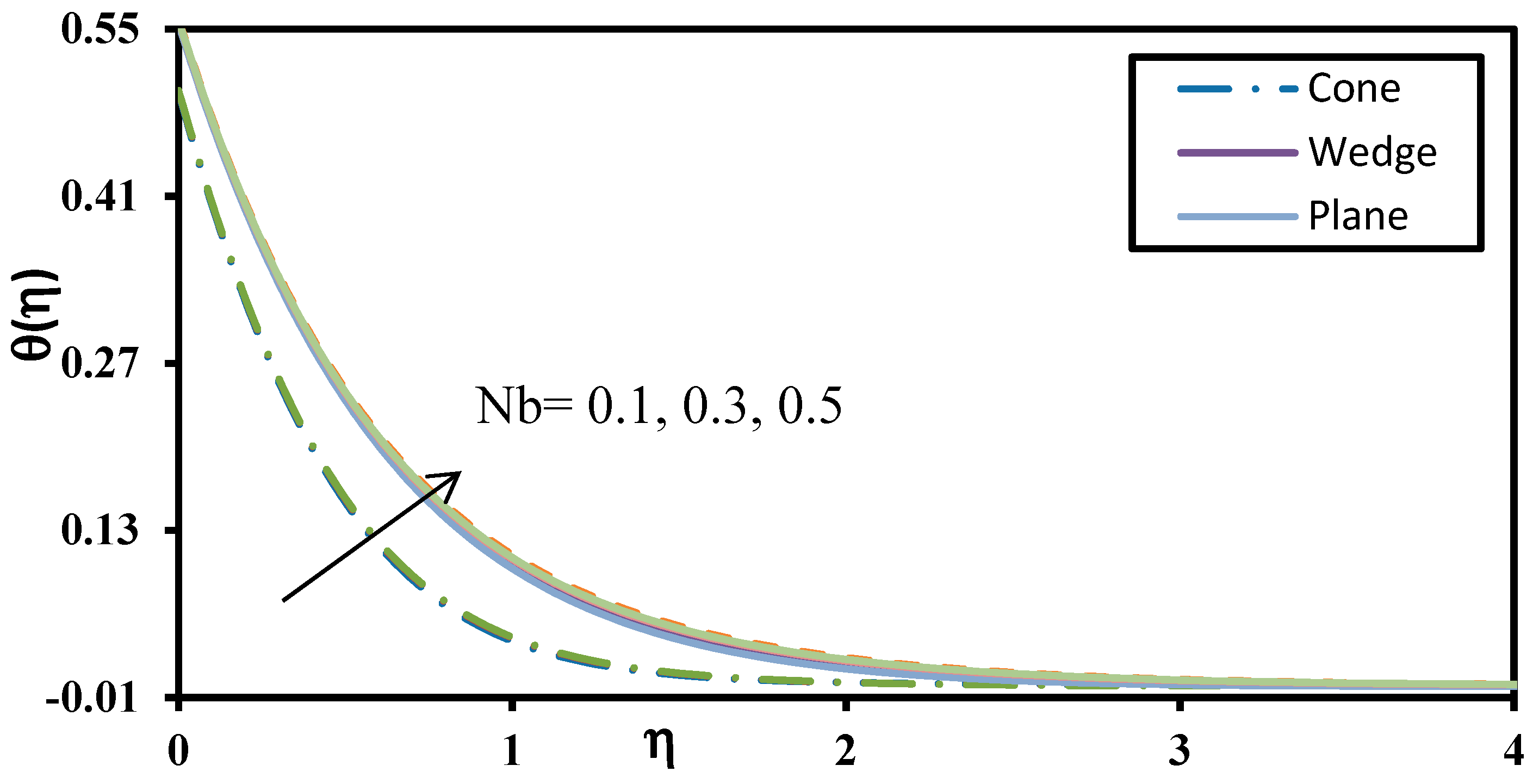
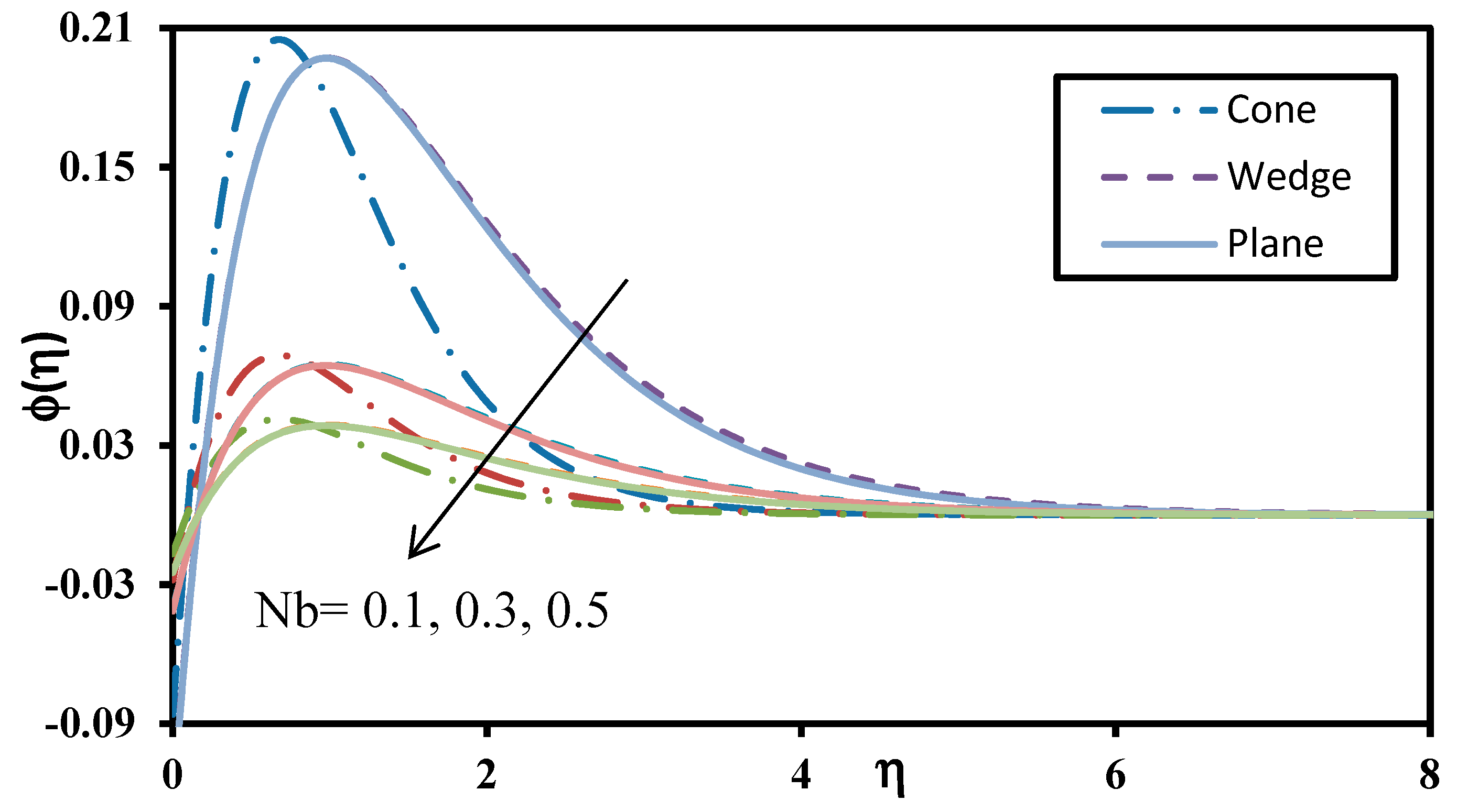
Figure 30 and Figure 31 illustrate the effect of Brownian motion parameter on temperature and nanoparticle volume fraction for different geometries. An increase in N b enhances the temperature profile while it evidently reduces the nanoparticle volume concentration. Increasing the Brownian motion parameter diminishes the nanoparticle diameter which encourages thermal diffusion and results in enhancement of heat transfer in the nanofluid as shown in Figure 30. In the Buongiorno model the parameter N b is inversely proportional to the size of nanoparticles (which are assumed spherical and homogenously distributed in the base fluid). With greater N b values smaller nanoparticles are present and this intensifies the thermal conduction heat transfer from the particles to the surrounding fluid (Figure 31). However, stronger Brownian motion inhibits the diffusion of nanoparticles since smaller nanoparticles are less successful in migrating through the base fluid and are more susceptible to ballistic collisions, as noted by Shukla and Dhir [54]. Physically excessive concentrations of nanoparticles (higher volume fractions) are counter-productive in nano-coating design and intermediate sized nanoparticles have been shown to disperse more homogenously. Thermal and nanoparticle concentration boundary layer thicknesses for the wedge exceed those achieved for the cone but are less than those for the plate.
Table 4, Table 5 and Table 6 displays the effect of parameters on skin factor, Nusselt number and Sherwood number for cone, wedge and plate respectively. In all the geometries, each afore-mentioned parameter exhibited the same behaviour. It can be observed from the tables that a rise in Brownian motion, Schmidt number and wall concentration parameter, reduces the Nusselt number while the other parameters enhance Nusselt number (heat transfer rate). Thermal and solutal Grashof numbers enhance the heat and mass transfer rates. Increasing wall temperature r 1 and concentration parameter r 2 reduce the skin friction coefficient. However, friction factor and reduced mass transfer rate defined by Equation (11) are increased whereas heat transfer rate is reduced with an increase in Schmidt number.

5. Conclusions

The present study investigates the external incompressible, steady-state boundary layer flow, heat and mass transfer behaviour in non-Newtonian power-law dilute nanofluid flow from three different over geometries (cone, wedge and plate) in the presence of variable wall thermal and solutal characteristics and wall transpiration. The effect of convective boundary conditions is considered and the revised Buongiorno nanofluid model is also deployed with focus on thermophoretic body forces and Brownian motion. The conservation equations are transformed with appropriate similarity variables and the resulting non-dimensional, nonlinear boundary value problems are solved using robust homotopy analysis method. The major findings of the study can be summarized as follows:
  • Momentum boundary layer thickness is more significantly modified for the plate compared to the cone and wedge whereas thermal and concentration boundary layer is more significantly altered for the wedge geometry.
  • Due to the boundary condition defined by modified Buongiorno model, the mass transfer rate (Sherwood number) decreases with increase in thermophoresis parameter and increases with increase in Brownian motion parameter for all the geometries.
  • Brownian motion exerts a stronger influence on mass transfer rates (Sherwood numbers) for all the geometries when compared to heat transfer rates (Nusselt numbers).
  • Increasing thermal Grashof number and solutal (nanoparticle) Grashof number reduce temperature and enhance wall heat transfer rates (Nusselt numbers).
  • Increasing thermal Grashof number and solutal (nanoparticle) Grashof number both elevate the skin friction factor for all geometries considered (cone, wedge and plate).
  • The Nusselt number for the cone is in excess of that for either a plate or wedge.
  • The convective boundary condition parameter, i.e., Biot number, controls the thermal and concentration boundary layer significantly and improves the heat transfer rates (Nusselt numbers) and in particular achieves high magnitudes for the wedge (Falkner–Skan case).
  • Increasing non-isothermal behaviour (rising value of wall temperature parameter) and non-iso-solutal effect (greater wall concentration parameter) magnifies the heat transfer and mass transfer rates (i.e., Nusselt and Sherwood numbers) for all geometries.
  • Thermal and solute Grashof number enhances the momentum boundary layer and suppresses the thermal and concentration boundary layer for all geometries. Both thermal and species buoyancy force therefore increase the rate of heat and nanoparticle mass transfer to the wall.
  • The dominant effect of increasing Schmidt number is to lessen the heat transfer rate and enhance skin friction and nanoparticle mass transfer rate for all geometries.
  • Increasing Schmidt number, Brownian motion and non-iso-solutal wall parameter deplete the Nusselt numbers, i.e., reduce heat transfer rates at the walls of all the geometries studied.
The present investigation has revealed some interesting insights into nanofluid transport characteristics in boundary layer flows from multiple geometries. However, it has been restricted to Fourier thermal conduction models. Future studies will consider thermal relaxation effects which may be simulated with non-Fourier models [55,56] and will be communicated imminently.

Author Contributions

Conceptualization, A.K.R., B.V., P.V.S.N.M., methodology, A.K.R., O.A.B., B.V., R.S.R.G., software, A.K.R. and O.A.B., validation, A.K.R., B.V., O.A.B. and P.V.S.N.M., formal analysis, A.K.R., B.V., investigation, A.K.R., O.A.B., resources, A.K.R., B.V., data curation, A.K.R., B.V., P.V.S.N.M., writing—review and editing, A.K.R., B.V., O.A.B., supervision, B.V.

Funding

The authors are grateful to Science and Engineering Research Board (SERB), Department of Science and Technology (DST), Govt of India for undertaking the research work under the research project file Number: ECR/2017/001053 dated 12/03/2018.

Acknowledgments

The authors are thankful to the reviewers for their useful and constructive comments which have helped to improve the present article.

Conflicts of Interest

The authors declare no conflict of interest.

References

  1. Roy, S. Free convection from a vertical cone at high Prandtl number. J. Heat Transf. 1974, 96, 115–117. [Google Scholar]
  2. Vajravelu, K.; Nayfeh, J. Hydromagnetic convection at a cone and a wedge. Int. Commun. Heat Mass Transf. 1992, 19, 701–710. [Google Scholar]
  3. Ramanaiah, G.; Malarvizhi, G. Free convection about a wedge and a cone subjected to mixed thermal boundary conditions. Acta Mech. 1992, 93, 119–123. [Google Scholar]
  4. Watanabe, T.; Funazaki, K.; Taniguchi, H. Theoretical analysis on mixed convection boundary layer flow over a wedge with uniform suction or injection. Acta Mech. 1994, 105, 133–141. [Google Scholar]
  5. Fang, T.; Lee, C.F. A moving-wall boundary layer flow of a slightly rarefied gas free stream over a moving flat plate. Appl. Math. Lett. 2005, 18, 487–495. [Google Scholar] [Green Version]
  6. Xu, H.; Liao, S.J. Laminar flow and heat transfer in the boundary-layer of non-Newtonian fluids over a stretching flat sheet. Comput. Math. Appl. 2009, 57, 1425–1431. [Google Scholar] [Green Version]
  7. Cheng, C.Y. Natural convection heat and mass transfer from a vertical truncated cone in a porous medium saturated with a non-Newtonian fluid with variable wall temperature and concentration. Int. Commun. Heat Mass Transf. 2009, 36, 585–589. [Google Scholar]
  8. Gorla, R.S.R.; Chamkha, A.J.; Rashad, A.M. Mixed convective boundary layer flow over a vertical wedge embedded in a porous medium saturated with a nanofluid: Natural convection dominated regime. Nanoscale Res. Lett. 2011, 6, 207–216. [Google Scholar]
  9. Rahman, M.M.; Lawatia, M.A.A.; Eltayeb, I.A.; Salti, N.A. Hydromagnetic slip flow of water based nanofluids past a wedge with convective surface in the presence of heat generation or absorption. Int. J. Therm. Sci. 2012, 57, 172–182. [Google Scholar]
  10. Chamkha, A.J.; Rashad, A.M. Unsteady heat and mass transfer by MHD mixed convection flow from a rotating vertical cone with chemical reaction and Soret and Dufour effects. Can. J. Chem. Eng. 2014, 92, 758–767. [Google Scholar]
  11. Rashidi, M.M.; Rastegari, M.T.; Asadi, M.; Bég, O.A. A study of non-Newtonian flow and heat transfer over a non-isothermal wedge using the homotopy analysis method. Chem. Eng. Commun. 2012, 199, 231–256. [Google Scholar]
  12. Vasu, B.; Kumar, M. Transient boundary layer laminar free convective flow of a nanofluid over a vertical cone/plate. Int. J. Appl. Comput. Math. 2015, 1, 427–448. [Google Scholar]
  13. Vasu, B.; Gorla, R.S.R. Two-phase laminar mixed convection Al2O3 water nanofluid in elliptic duct. Nanoscale Flow Adv. Model. Appl. 2015, 4, 101–120. [Google Scholar]
  14. Vasu, B.; Gorla, R.S.R.; Murthy, P.V.S.N. Thermophoresis on boundary layer heat and mass transfer flow of Walters-B fluid past a radiate plate with heat sink/source. Heat Mass Transf. 2017, 53, 1553–1570. [Google Scholar]
  15. Vasu, B.; Gorla, R.S.R.; Murthy, P.V.S.N.; Bég, O.A.; Prasad, V.R.; Kadir, A. Unsteady flow of a nanofluid over a sphere with non-linear Boussinesq approximation. AIAA J. Thermophys. Heat Transf. 2018. [Google Scholar] [CrossRef]
  16. Ray, A.K.; Vasu, B.; Bég, O.A.; Gorla, R.S.R.; Murthy, P.V.S.N. Magneto-bioconvection flow of a Casson thin film with nanoparticles over an unsteady stretching sheet. Int. J. Numer. Methods Heat Fluid Flow 2019. [Google Scholar] [CrossRef]
  17. Sreenivasulu, P.; Vasu, B.; Tamalapakula, P.; Reddy, N.B. Inclined Lorentzian force effect on tangent hyperbolic radiative slip flow imbedded carbon nanotubes: Lie group analysis. J. Comput. Appl. Res. Mech. Eng. 2018. [Google Scholar] [CrossRef]
  18. Irgens, F. Rheology and Non-Newtonian Fluids; Springer International Publishing: New York, NY, USA, 2014. [Google Scholar]
  19. Prasad, V.R.; Vasu, B.; Bég, O.A.; Parshad, R. Unsteady free convection heat and mass transfer in a Walters-B viscoelastic flow past a semi-infinite vertical plate: A numerical study. Therm. Sci. 2011, 15, 291–305. [Google Scholar]
  20. Ray, A.K.; Vasu, B. Hydrodynamics of non-Newtonian Spriggs fluid flow past an impulsively moving plate. In Applications of Fluid Dynamics; Springer: Singapore, 2018; pp. 95–107. [Google Scholar]
  21. Chhabra, R.P.; Richardson, J. Non-Newtonian Flow and Applied Rheology: Engineering Applications, 2nd ed.; Butterworth-Heinemann: Oxford, UK, 2008. [Google Scholar]
  22. Acrivos, A.; Shah, M.J.; Petersen, E.E. Momentum and heat transfer in laminar boundary-layer flows of non-Newtonian fluids past external surfaces. AIChE J. 1960, 6, 312–317. [Google Scholar]
  23. Schowalter, W.R. The application of boundary-layer theory to power-law pseudoplastic fluids: Similar solutions. AIChE J. 1960, 6, 24–28. [Google Scholar]
  24. Gorla, R.S.R.; Kumari, M. Non-similar solutions for mixed convection in non-Newtonian fluids along a vertical plate in a porous medium. Transp. Porous Med. 1998, 33, 295–307. [Google Scholar]
  25. Ikbal, M.A.; Chakravarty, S.; Wong, K.K.; Mazumdar, J.; Mandal, P.K. Unsteady response of non-Newtonian blood flow through a stenosed artery in magnetic field. J. Comput. Appl. Math. 2009, 230, 243–259. [Google Scholar]
  26. Mahapatra, T.R.; Nandy, S.K.; Gupta, A.S. Heat transfer in the magneto hydrodynamic flow of a power-law fluid past a porous flat plate with suction or blowing. Int. Commun. Heat Mass Transf. 2012, 39, 17–23. [Google Scholar]
  27. Qi, Z.; Kuang, S.; Rong, Y.A. Lattice Boltzmann investigation of the wake effect on the interaction between particle and power-law fluid flow. Powder Technol. 2018, 326, 208–221. [Google Scholar]
  28. Vasu, B. MHD free convection flow of power-law nanofluid film along an inclined surface with viscous dissipation and joule heating. World J. Eng. 2019, 16, 115–124. [Google Scholar]
  29. Bég, O.A.; Malleque, K.A.; Islam, M.N. Modelling of Ostwald-deWaele non-Newtonian flow over a rotating disk in a non-Darcian porous medium. Int. J. Appl. Math. Mech. 2012, 8, 46–67. [Google Scholar]
  30. Choi, U.S.; Eastman, J.A. Enhancing Thermal Conductivity of Fluids with Nanoparticles; Argonne National Lab.: Lemont, IL, USA, 1995. [Google Scholar]
  31. Buongiorno, J. Convective transport in nanofluids. ASME J. Heat Transf. 2006, 128, 240–250. [Google Scholar]
  32. Minkowycz, W.J.; Sparrow, E.M.; Abraham, J.P. Nanoparticle Heat Transfer and Fluid Flow; CRC press: Boca Raton, FL, USA, 2016. [Google Scholar]
  33. Xuan, Y.; Roetzel, W. Conceptions for heat transfer correlation of nanofluids. Int. J. Heat Mass Transf. 2000, 43, 3701–3707. [Google Scholar]
  34. Godson, L.; Raja, B.; Lal, D.M.; Wongwises, S. Enhancement of heat transfer using nanofluids—An overview. Renew. Sustain. Energy Rev. 2010, 14, 629–641. [Google Scholar]
  35. Yacob, N.A.; Ishak, A.; Nazar, R.; Pop, I. Falkner-Skan problem for a static and moving wedge with prescribed surface heat flux in a nanofluid. Int. Commun. Heat Mass Transf. 2011, 38, 149–153. [Google Scholar]
  36. Kuznetsov, A.V.; Nield, D.A. Natural convective boundary-layer flow of a nanofluid past a vertical plate. Int. J. Therm. Sci. 2010, 49, 243–247. [Google Scholar]
  37. Bachok, N.; Ishak, A.; Pop, I. Boundary-layer flow of nanofluids over a moving surface in a flowing fluid. Int. J. Therm. Sci. 2010, 49, 1663–1668. [Google Scholar]
  38. Bég, O.A.; Prasad, V.R.; Vasu, B. Numerical study of mixed bioconvection in porous media saturated with nanofluid containing oxytactic microorganisms. J. Mech. Med. Biol. 2013, 13, 1350067. [Google Scholar]
  39. Kuznetsov, A.V.; Nield, D.A. Natural convective boundary-layer flow of a nanofluid past a vertical plate: A revised model. Int. J. Therm. Sci. 2014, 77, 126–129. [Google Scholar]
  40. Malvandi, A.; Ganji, D.D. Brownian motion and thermophoresis effects on slip flow of alumina/water nanofluid inside a circular microchannel in the presence of a magnetic field. Int. J. Therm. Sci. 2014, 84, 196–206. [Google Scholar]
  41. Moshizi, S.A.; Malvandi, A.; Ganji, D.D.; Pop, I. A two-phase theoretical study of Al2O3–water nanofluid flow inside a concentric pipe with heat generation/absorption. Int. J. Therm. Sci. 2014, 84, 347–357. [Google Scholar]
  42. Kameswaran, P.K.; Vasu, B.; Murthy, P.V.S.N.; Gorla, R.S.R. Mixed convection from a wavy surface embedded in a thermally stratified nanofluid saturated porous medium with non-linear Boussinesq approximation. Int. Commun. Heat Mass 2016, 77, 78–86. [Google Scholar]
  43. Bég, O.A.; Basir, M.F.M.; Uddin, M.J.; Ismail, A.M. Numerical study of slip effects on unsteady asymmetric bioconvective nanofluid flow in a porous microchannel with an expanding/contracting upper wall using Buongiorno’s model. J. Mech. Med. Biol. 2017, 17, 1750059. [Google Scholar]
  44. Liao, S. Homotopy Analysis Method in Nonlinear Differential Equations; CRC Press: Boca Raton, FL, USA, 2011. [Google Scholar]
  45. Bataineh, A.S.; Noorani, M.S.M.; Hashim, I. Approximate analytical solutions of systems of PDEs by homotopy analysis method. Comput. Math Appl. 2008, 55, 2913–2923. [Google Scholar] [Green Version]
  46. Sheikholeslami, M.; Nimafar, M.; Ganji, D.D. Analytical approach for the effect of melting heat transfer on nanofluid heat transfer. Eur. Phys. J. Plus 2017, 132, 385. [Google Scholar]
  47. Mabood, F.; Khan, W.A.; Ismail, A.M. MHD flow over exponential radiating stretching sheet using homotopy analysis method. J. King Saud Univ. Eng. Sci. 2017, 29, 68–74. [Google Scholar]
  48. Sravanthi, C.S.; Gorla, R.S.R. Effects of heat source/sink and chemical reaction on MHD Maxwell nanofluid flow over a convectively heated exponentially stretching sheet using homotopy analysis method. Int. J. Appl. Mech. Eng. 2018, 23, 137–159. [Google Scholar]
  49. Hayat, T.; Kiran, A.; Imtiaz, M.; Alsaed, A. Unsteady flow of carbon nanotubes with chemical reaction and Cattaneo-Christov heat flux model. Nonlinear Anal. Real World Appl. 2009, 10, 2346–2356. [Google Scholar]
  50. Bég, O.A.; Tasveer, A.; Rashidi, M.M.; Asadi, M. Homotopy semi-numerical modelling of nanofluid convection flow from an isothermal spherical body in a permeable regime. Int. J. Microscale Nanoscale Therm. Fluid Transp. Phenom. 2012, 3, 237–266. [Google Scholar]
  51. Bég, O.A.; Rashidi, M.M.; Rahimzadeh, N.; Tasveer, A.; Hung, T.K. Homotopy semi-numerical simulation of two-phase thermal haemodynamics in a high permeability blood purification device. J. Mech. Med. Biol. 2013, 13, 1350066. [Google Scholar]
  52. Ray, A.K.; Vasu, B.; Gorla, R.S.R. Homotopy simulation of non-Newtonian spriggs fluid flow over a flat plate with oscillating motion. Int. J. Appl. Mech. Eng. 2019, 24, 359–385. [Google Scholar]
  53. Hassanien, I.A.; Abdullah, A.A.; Gorla, R.S.R. Flow and heat transfer in a power-law fluid over a non-isothermal stretching sheet. Math. Comput. Model. 1998, 28, 105–116. [Google Scholar]
  54. Shukla, R.K.; Dhir, V.K. Effect of Brownian motion on thermal conductivity of nanofluids. ASME J. Heat Transf. 2008, 130, 042406. [Google Scholar]
  55. Vasu, B.; Ray, A.K. Numerical study of Carreau nanofluid flow past vertical plate with the Cattaneo–Christov heat flux model. Int. J. Numer. Methods Heat Fluid Flow 2019, 29, 702–723. [Google Scholar]
  56. Mishra, S.R.; Shamshuddin, M.; Bég, O.A.; Kadir, A. Numerical study of heat transfer and viscous flow in a dual rotating extendable disk system with a non-Fourier heat flux model. Heat Transf. Asian Res. 2018. [Google Scholar] [CrossRef]
Figure 1. Geometry Configuration.
Inventions 04 00054 g001
Figure 2. h -curve.
Figure 2. h -curve.
Inventions 04 00054 g002
Figure 3. Effect of Newtonian and non-Newtonian fluid over velocity for different geometries.
Inventions 04 00054 g003
Figure 4. Effect of Newtonian and non-Newtonian fluid over temperature for different geometries.
Inventions 04 00054 g004
Figure 5. Effect of Newtonian and non-Newtonian fluid over nanoparticle volume fraction.
Inventions 04 00054 g005
Figure 6. Effect of thermal Grashof number over velocity profile.
Inventions 04 00054 g006
Figure 7. Effect of thermal Grashof number over temperature profile.
Inventions 04 00054 g007
Figure 8. Effect of thermal Grashof number over nanoparticle volume fraction.
Inventions 04 00054 g008
Figure 9. Effect of solute Grashof number over velocity profile.
Inventions 04 00054 g009
Figure 10. Effect of solute Grashof number over temperature profile.
Inventions 04 00054 g010
Figure 11. Effect of solute Grashof number over nanoparticle volume fraction profile.
Inventions 04 00054 g011
Figure 12. Effect of suction/blowing on velocity.
Inventions 04 00054 g012
Figure 13. Effect of suction/blowing on temperature.
Inventions 04 00054 g013
Figure 14. Effect of suction/blowing on nanoparticle volume fraction.
Inventions 04 00054 g014
Figure 15. Effect of wall temperature parameter on velocity.
Inventions 04 00054 g015
Figure 16. Effect of wall temperature parameter on temperature.
Inventions 04 00054 g016
Figure 17. Effect of wall temperature parameter on nanoparticle volume fraction.
Inventions 04 00054 g017
Figure 18. Effect of wall concentration parameter on velocity.
Inventions 04 00054 g018
Figure 19. Effect of wall concentration parameter on temperature.
Inventions 04 00054 g019
Figure 20. Effect of wall concentration parameter on nanoparticle volume fraction.
Inventions 04 00054 g020
Figure 21. Effect of Prandtl number on velocity profile for different geometries.
Inventions 04 00054 g021
Figure 22. Effect of Prandtl number on temperature profile for different geometries.
Inventions 04 00054 g022
Figure 23. Effect of Biot number on velocity profile for different geometries.
Inventions 04 00054 g023
Figure 24. Effect of Biot number on temperature profile for different geometries.
Inventions 04 00054 g024
Figure 25. Effect of Biot number on nanoparticle volume fraction profile for different geometries.
Inventions 04 00054 g025
Figure 26. Effect of Schmidt number on velocity profile for different geometries.
Inventions 04 00054 g026
Figure 27. Effect of Biot number on nanoparticle volume fraction profile for different geometries.
Inventions 04 00054 g027
Figure 28. Effect of thermophoresis parameter on temperature profile for different geometries.
Inventions 04 00054 g028
Figure 29. Effect of thermophoresis parameter on concentration profile for different geometries.
Inventions 04 00054 g029
Figure 30. Effect of Brownian motion parameter on temperature profile for different geometries.
Inventions 04 00054 g030
Figure 31. Effect of Brownian motion parameter on concentration profile for different geometries.
Inventions 04 00054 g031
Table 1. Convergence of HAM solution.
m (Order)f″(0)θ′(0)ϕ′(0)
4−1.03007−0.892450.89245
8−1.03696−0.972440.97244
10−1.03724−0.989550.98955
12−1.03712−0.999060.99906
16−1.03673−1.00664−1.00665
20−1.03651−1.008221.00822
22−1.03658−1.008291.00829
Table 2. Comparison of the present study for f ( 0 ) at n = 1 ,   G r = G c = 0 for different S.
SExact [53]Hassanien et al. [53]Present
−1.50.5000050.5000050.500093
−10.6180420.6180420.6179949
−0.50.7807810.7807810.7807835
01.000001.000001.000000
0.51.2807771.2807771.280275
11.6180341.6180341.616967
1.52.000002.00000−1.99857
Table 3. Computational time and order of variation with respect to different residual error in temperature for the various geometries.
GeometriesResidual ErrorOrder Computational Time (in Seconds)
Cone10−344.1638
10−5610.8407
10−71276.2564
Wedge10−320.758698
10−568.5965
10−71267.8979
Plate10−320.75515
10−543.2184
10−71041.0949
Table 4. Effect of different parameters on skin factor, Nusselt number and Sherwood number for Cone.
Pr G r G c S r 1 r 2 S c N t N b γ C f N u S h
1 1.04838450.780282−0.78028
2 1.11430021.00665−1.00665
5 1.1642961.26109−1.26109
10 1.17017141.006335−1.00634
0.5 1.11430021.00665−1.00665
1 1.05794791.007142−1.00714
0.50 1.1883451.002249−1.00225
0.5 1.11430021.00665−1.00665
1 1.04638521.011312−1.01131
0.50 0.95537580.942301−0.9423
0.2 1.28243391.06812−1.06812
0.4 1.63628231.178777−1.17878
0.10 1.09423660.878849−0.87885
0.5 1.10530630.949277−0.94928
1 1.11430021.00665−1.00665
0 1.0963991.007789−1.00779
0.5 1.10658141.007163−1.00716
1 1.11430021.00665−1.00665
1 1.14242731.007178−1.00718
2 1.07136181.00337−1.00337
3 1.05761911.000187−1.00019
1.20.1 1.11430021.00665−1.00665
0.3 0.98154061.007427−3.02228
0.5 0.86718231.0101−5.0505
0.10.1 1.11430021.00665−1.00665
0.3 1.16295071.003694−0.33456
0.5 1.17302161.003114−0.20062
0.111.15775630.670264−0.67026
21.11430021.00665−1.00665
41.0727421.341994−1.34199
Table 5. Effect of different parameters on skin factor, Nusselt number and Sherwood number for Wedge.
Pr G r G c S r 1 r 2 S c N t N b γ C f N u S h
1 0.6733890.682206−0.682206
2 0.7317890.888087−0.888087
5 0.7843821.128502−1.128502
10 0.8214040.883647−0.883647
0.5 0.7317890.888087−0.888087
1 0.6478590.891888−0.891888
0.50 0.7968720.88223−0.88223
0.5 0.7317890.888087−0.888087
1 0.6707130.894365−0.894365
0.50 0.6624370.852889−0.852889
0.2 0.8059170.923339−0.923339
0.4 0.967380.993094−0.993094
0.10 0.6922450.665117−0.665117
0.5 0.7154190.79364−0.79364
1 0.7317890.888087−0.888087
0 0.7278550.888483−0.888482
0.5 0.727460.888416−0.888416
1 0.7317890.888087−0.888087
1 0.7692990.886881−0.886881
2 0.662770.888964−0.888963
3 0.6313570.888297−0.88829
1.20.1 0.7317890.888087−0.888087
0.3 0.6110190.893689−2.681066
0.5 0.50120.901164−4.505822
0.10.1 0.7317890.888087−0.888087
0.3 0.7746660.884138−0.294713
0.5 0.7834820.88337−0.176674
0.110.7777080.614742−0.614742
20.7317890.888087−0.888087
40.6919191.141768−1.141768
Table 6. Effect of different parameters on skin factor, Nusselt number and Sherwood number for Plate.
Pr G r G c S r 1 r 2 S c N t N b γ C f N u S h
1 0.59670380.689775−0.68978
2 0.67190770.892232−0.89223
5 0.74214221.130564−1.13056
10 0.79256170.886282−0.88628
0.5 0.67190770.892232−0.89223
1 0.56088910.896999−0.897
0.50 0.75875740.883975−0.88398
0.5 0.67190770.892232−0.89223
1 0.59267990.901358−0.90136
0.50 0.60561810.857314−0.85731
0.2 0.74357050.927157−0.92716
0.4 0.90235290.996141−0.99614
0.10 0.6194370.669709−0.66971
0.5 0.66565020.892576−0.89258
1 0.67190770.892232−0.89223
0 0.6662160.892418−0.89242
0.5 0.66565020.892576−0.89258
1 0.67190770.892232−0.89223
1 0.72201570.890116−0.89012
2 0.58162180.894629−0.89463
3 0.54127320.894543−0.89454
1.20.1 0.67190770.892232−0.89223
0.3 0.51660010.904096−2.71229
0.5 0.37884740.920086−4.60043
0.10.1 0.67190770.892232−0.89223
0.3 0.72876650.886638−0.29555
0.5 0.74062240.885563−0.17711
0.110.73345580.616243−0.61624
20.67190770.892232−0.89223
40.61928471.149904−1.1499

