Proposed Smart Monitoring System for the Detection of Bee Swarming

Abstract

This paper presents a bee-condition-monitoring system incorporated with a deep-learning process to detect bee swarming. This system includes easy-to-use image acquisition and various end node approaches for either on-site or cloud-based mechanisms. This system also incorporates a new smart CNN engine called Swarm-engine for detecting bees and the issue of notifications in cases of bee swarming conditions to the apiarists. First, this paper presents the authors’ proposed implementation system architecture and end node versions that put it to the test. Then, several pre-trained networks of the authors’ proposed CNN Swarm-engine were also validated to detect bee-clustering events that may lead to swarming. Finally, their accuracy and performance towards detection were evaluated using both cloud cores and embedded ARM devices on parts of the system’s different end-node implementations.

1. Introduction

The Internet of Things (IoT) industry is shifting fast towards the agricultural sector, aiming for the vast applicability of new technologies. Existing applications in agriculture include environmental monitoring of open field agricultural systems, the food supply chain monitoring, and livestock monitoring [1,2,3,4]. Several bee-monitoring and beekeeping-resource management systems or frameworks that incorporate IoT and smart services have been proposed in the literature [5,6,7], while others exist as market solutions. This paper investigates existing technological systems focusing on detecting bee stress, queen succession, or Colony Collapse Disorder (CCD), favorable conditions that can lead to bee swarming. Swarming is when honeybee colonies reproduce to form new ones or when a honeybee colony becomes too congested or stressed and requires beekeeping treatments.

Swarming is the phenomenon of bee clustering that indicates a crowded beehive that usually appears under normal conditions. At its first development stages, it seems at the end frame of the brood box or in the available space between the upper part of the frames and the beehive lid.

In most cases, bee swarming is a natural phenomenon that beekeepers are called to mitigate with new frames or floors. Nevertheless, in many cases, bee clustering events that lead to bee swarming may occur in cases such as: (a) Varroa mite disease outbursts that lead to the replacement of the queen, (b) the birth of a new queen, which takes part of the colony and abandons the beehive, or (c) extreme environmental conditions or even low pollen supplies, which decrease the queen’s laying and force her to migrate. All of the above cases (a),(b), and (c) lead to swarming events. The following paragraphs describe how the variation of the condition parameters can lead to swarming events.

The environment inside and around the beehives is vital to the colony establishment’s success and development. An essential factor in apiary hives that affects both colony survival and honey yield is the ability to manage agricultural interventions and disease treatments (especially Varroa mite [8]) and monitor the conditions inside the beehive [9,10,11].

Beehive colonies are especially vulnerable to temperature fluctuations, which in turn affect honey yields. At high temperatures above 35 °C, honeybees are actively involved in the thermoregulation of the colony with fanning activities. For low temperatures below 15 °C, they reduce their mobility and gather at the center of the brood box, forming bee clusters and consuming collected honey [5,12]. Regarding the air temperature inside the beehives, a mathematical model was presented in [13]. Moreover, bee swarming is also strongly correlated with temperature variations [14]. Therefore, to alleviate temperature stress events, inexpensive autonomous temperature-monitoring devices [15] and IoT low-power systems have been proposed in the literature. Such systems are the WBee system [16], an RF temperature monitoring system with GPS capabilities presented in [14], the BeeQ Resources Management System [17], and the SBMaCS, which utilizes piezoelectric-energy-harvesting functionalities for temperature measurements’ data transmissions [18].

Similarly, high humidity levels can lead to swarming events inside the beehive, excessive colony honey consumption, and the production of propolis and wax by the bees as a countermeasure [19,20]. Beehive humidity levels’ reduction concerning atmospheric humidity is achieved with the opening/closing of the ventilation holes attached to the beehive lid [21], or with the use of automated blower fans [22], or integrated Peltier systems [12].

The use of weight scales with the adoption of resource-monitoring systems and treatment protocols may also be of assistance to mitigate swarming events based on colony strength, and constitution [23]. It has been reported that significant weight reduction for a fully deployed ten-frame beehive cell below 19 kg indicates swarming in progress requiring immediate attention and feeding interventions, as confirmed by apiarists.

Apart from temperature, humidity, and weight monitoring, sound monitoring has also been proposed to detect swarming events, as provided by the analysis in [24]. The authors in [25] classified the swarming spectrum at 400–500 Hz with a duration interval of at least 35 min. Using Mel Frequency Cepstral Coefficients (MFCCs) and deltas, as well as Mel band spectra computational sound scene analysis, the authors in [26], tried to detect coefficients that denote swarming. The authors in [27] used MFCC feature coefficient vectors and trained a system using the Gaussian Mixture Model (GMM) and Hidden Markov Model (HMM) classifiers to detect swarming. Furthermore, the authors in [28] proposed a support vector machine classifier of MFCC coefficients and a CNN model that can also be used for swarm detection.

Beehive cameras in beekeeping have been used mainly as a security and antitheft protection instrument rather than a condition-monitoring one. Nevertheless, significant steps over the last few years have been taken, using mainly image-processing techniques, circular Hough transformations [29], background subtractions, and eclipse approximations, to detect bees or bee flying paths at the hive entrances [30]. Apart from image processing, another system used for bee counting using IR sensors at the beehive entrances was presented in [31]. Image processing is the easiest to implement and most reliable source for swarming or external attack alert detection. Nevertheless, if performed at the hive entrance, it cannot reliably detect the occurring event early enough for the beekeepers to ameliorate it successfully.

Since swarming events occur mainly during the day and in the spring and summer months, as indicated by apiarists, this paper presents a new camera sensor system for detecting swarming inside the beehive. The proposed system uses a camera that incorporates an image-processing motion logic and utilizes a pre-trained Convolutional Neural Network (CNN) to detect bees. The rest of this paper is structured as follows: Section 2 presents related work in existing beehive-condition-monitoring products on the market. Section 3 presents the authors’ proposed monitoring system and the system’s capabilities. Section 4 presents the CNN algorithms used by the system and detection algorithm process. Section 5 presents the authors’ experimentation on different end node devices, CNN algorithms and models as well as real testing for bees detection and bee swarming. Finally, the paper summarizes the findings and experimental results of the system.

2. Related Work on Beehive-Condition-Monitoring Products

In this section, the relevant research is presented based on which devices have been used for monitoring and recording the bee swarming conditions that prevail at any given time inside the beehive cells. The corresponding swarming-detection services provided by each device are divided into three categories: (a) honey productivity monitoring using weight scales, image motion detection, or other sensors, (b) direct population monitoring using cameras and smart AI algorithms and deep neural networks, (c) indirect population monitoring only using audio, or other sensors, or cameras that are not located externally, or cameras without any smart AI algorithm for automated detection. The prominent representatives of the devices performing the population monitoring are the Bee-Shop Camera Kit [32] and the EyeSon [33] for Category (a) and the Zygi [34], Arnia [35], Hive-Tech [36], and HiveMind [37] devices for Category (c). On the other hand, no known devices on the market directly monitor beehives using cameras inside the beehive box (Category (b)).

Table 1. Existing bee-swarming-monitoring systems.

System/Device	Swarm-Monitoring Capabilities
	Productivity Monitoring	Indirect Population Monitoring Using Cameras	Indirect Population Monitoring Using Sound or Other Sensors
Bee-Shop camera kit [32]	✓	✓
HiveMind system [37]	✓		✓
Hive-Tech system [36]	✓		✓
Arnia system [35]	✓		✓
EyeSon Hive system [33]	✓	✓
Zygi [34]	✓	✓

summarizes existing beehive-monitoring systems concerning population monitoring and productivity.

The Bee-Shop [32] monitoring equipment can observe the hive’s productivity through video recording or photos. The monitoring device is placed in front of the beehive door. The captured material is stored on an SD card. It can be sent to the beekeeper’s mobile phone using the 3G/4G LTE network, showing the contours of bee swarms as detected from the image-detection algorithm included in the camera kit. Similarly, the Bee-Shop camera kit offers motion detection and security instances for the apiary.

Similarly, EyeSon Hives [33] uses an external bee box camera and an image-detection algorithm to record the swarms of bees located outside the hive and algorithmically analyze the swarm flight direction. EyeS on Hives [33] also uses 3G/4G LTE connectivity and enables the beekeeper to stream video via a mobile phone application in real-time.

Zygi [34] provides access to weight measurements. It is also capable of a variety of external measurements such as temperature and humidity. Nevertheless, since this is performed externally, such weight measurements do not indicate the conditions that apply inside the beehive box. Zygi also includes an external camera placed in front of the bee box and transmits photo snapshots via GSM or GPRS. However, this functionality does not have a smart engine or image-detection algorithm to detect swarming and requires beekeepers’ evaluation.

Devices similar to Zygi [34] are the Arnia [35], Hive-Tech [36], and HiveMind [37] devices, which are assumed to be indirect monitoring devices due to the absence of a camera module.

Hive-Tech [36] can monitor the bee box and detect swarming by using a monitoring IR sensor or reflectance sensors that detect real-time crowd conditions at the bee box openings (where the sensors are placed), as well as bee mobility and counting [38,39]. The algorithm used is relatively easy to implement, and swarming results can be derived using data analysis.

Arnia [35] includes a microphone with audio-recording capabilities, FFT frequency spikes, Mel Frequency Cepstral Coefficient (MFCC) deltas’ monitoring [28], and notifications. Finally, HiveMind [37] includes humidity and temperature sensors and a bee activity sound/IR sensor as a good indicator for overall beehive doorway activity.

3. Proposed Monitoring System

The authors propose a new incident-response system for automatic detection of swarming. The system includes the following components: (1) The Beehive-Monitoring Node, (2) The Quality Resource Management System and (3) The Beehive end node application. System components are described in the subsections that follow.

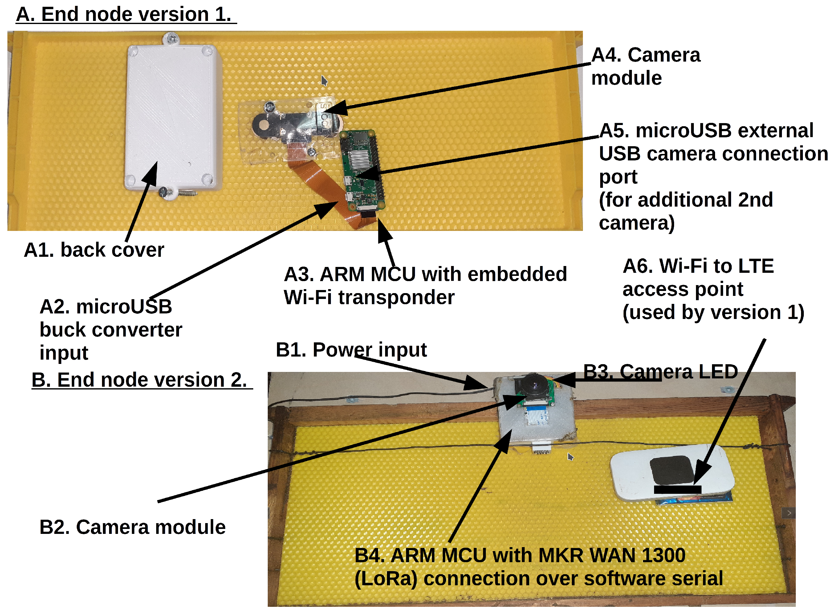
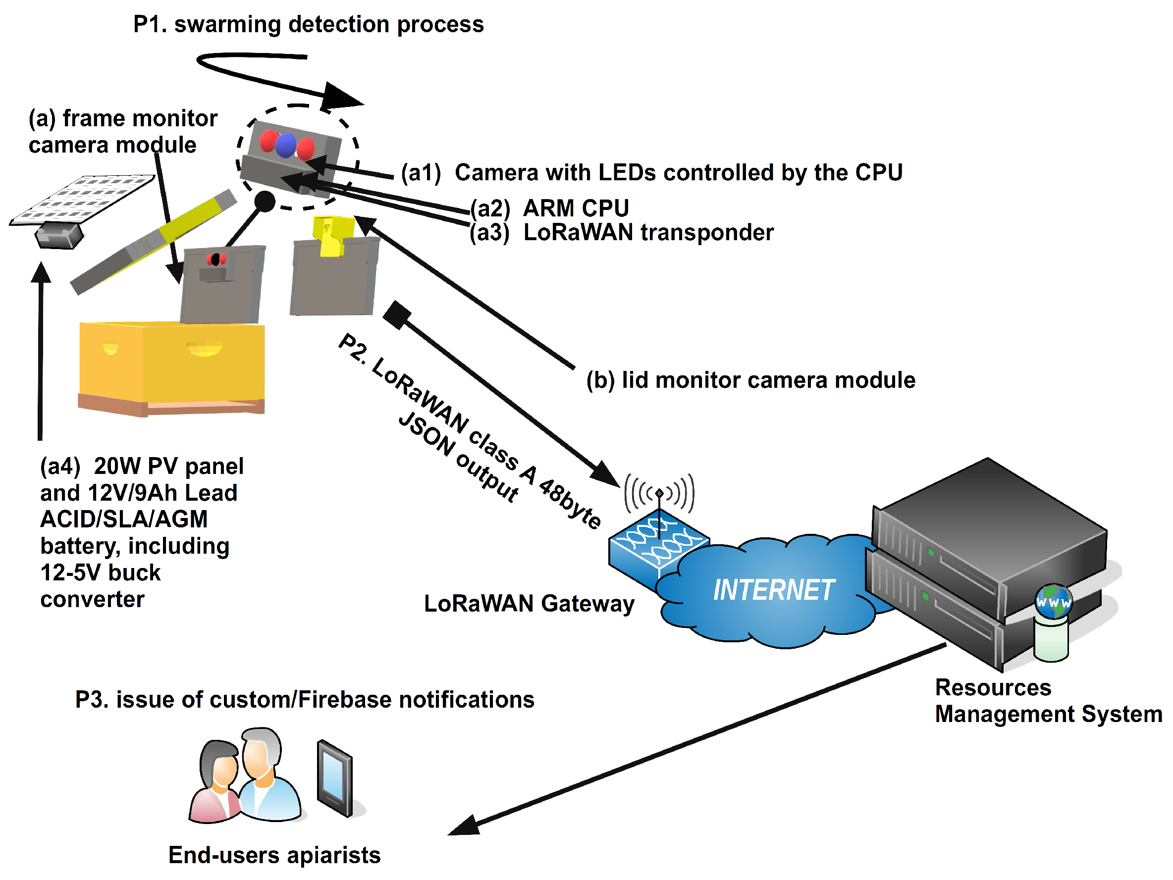
3.1. Beehive-Monitoring Node

The beehive-camera-monitoring node is placed inside the beehive’s brood box and includes the following components:

• The camera module component. The camera module component is responsible for the acquisition of still images inside the beehive. It is placed on a plastic frame covered entirely with a smooth plastic surface to avoid being built on or waxed by bees. The camera used is a fish-eye lens of a 180–200° view angle, a 5MPixel camera with LEDs included (brightness controlled by the MCU), and adjustable focus distance connected directly to the ARM using the MIPI CSI/2 interface using a 15 pin FFC cable. The camera module can take ultra-wide HD images of 2592 × 1944 resolution and achieve frame rates of 2 frames/s for single-core ARM, 8 frames/s for quad-core ARM, and 23 frames/s for octa-core ARM devices, at its maximum resolution potential
• The microprocessor control unit, responsible for storing camera snapshots and uploading them to the cloud (for Version 1 end node devices) or responsible for taking camera snapshots and implementing the deep-learning detection algorithm (for Version 2 end node devices)
• The network transponder device, which can be either a UART-connected WiFi transponder (for Version 1 nodes) or an ARM microprocessor, including an SPI connected LoRaWAN transponder (for Version 2 nodes)
• The power component, which includes a 20 W/12 V PV panel connected directly to a 12 V-9 Ah lead-acid SLA/AGM battery. The battery is placed under the PV panel on top of the beehive and feeds the ARM MCU unit using a 12-5 V/2 A buck converter. The battery used is a deep depletion one since the system might, due to its small battery capacity, be fully discharged, especially at night or on prolonged cloudy days

3.2. Beehive Concentrator

The concentrator is responsible for the nodes’ data transmission over the Internet to the central storage and management unit, called the Bee Quality Resource Management System. It acts as an intermediate gateway among the end nodes and the BeeQ RMS application service and web interface (see Figure A4). Depending on the version of the nodes, for node v1, the beehive concentrator is a Wi-Fi access point over the 3G/4G LTE cellular network, and Version 2 is a LoRaWAN gateway over 3G/4G LTE. Figure 1a,b illustrate the Node-1 and Node-2 devices and their connectivity to the RMS over the different types of beehive concentrators. The technical specifications and capabilities also differ among the two implementation versions.

The Version 1 node concentrator (see Figure 1) can upload images with an overall bandwidth capability that varies from 1–7/10–57 Mbps, depending on the gateway’s distance from the beehive and limited by the LTE technology used. Nevertheless, it is characterized as a close-distance concentrator solution since the concentrator must be inside the beehive array and at a LOS distance of no more than 100 m from the hive. The other problem with Version 1 node concentrators is that their continuous operation and control signaling transmissions waste 40–75% more energy than LoRaWAN [40].

For Version 2 devices, the LoRaWAN concentrator is permanently set to a listening state and can be emulated as a class-C single-channel device (see Figure 2). In such cases, for a 6 Ah battery, which can deliver all its potential, the expected gateway uptime is 35–40 h [41] (without calculating the concentrator’s LTE transponder energy consumption). The coverage distance of the Version 2 concentrator also varies since it can cover distances up to 12–18 km for Line Of Sight (LOS) setups and 1–5 km for non-LOS ones [42]. Furthermore, its scalability differs since it can deliver at least 100–250 nodes per concentrator at SF-12 and a worst-case packet loss of 10–25% [43], concerning a maximum of 5–10 nodes for the WiFi ones. The disadvantage of the Class-2 node is that its Bandwidth (BW) potential is limited to 0.3–5.4 Kbps, including the duty cycle transmission limitations [44]:

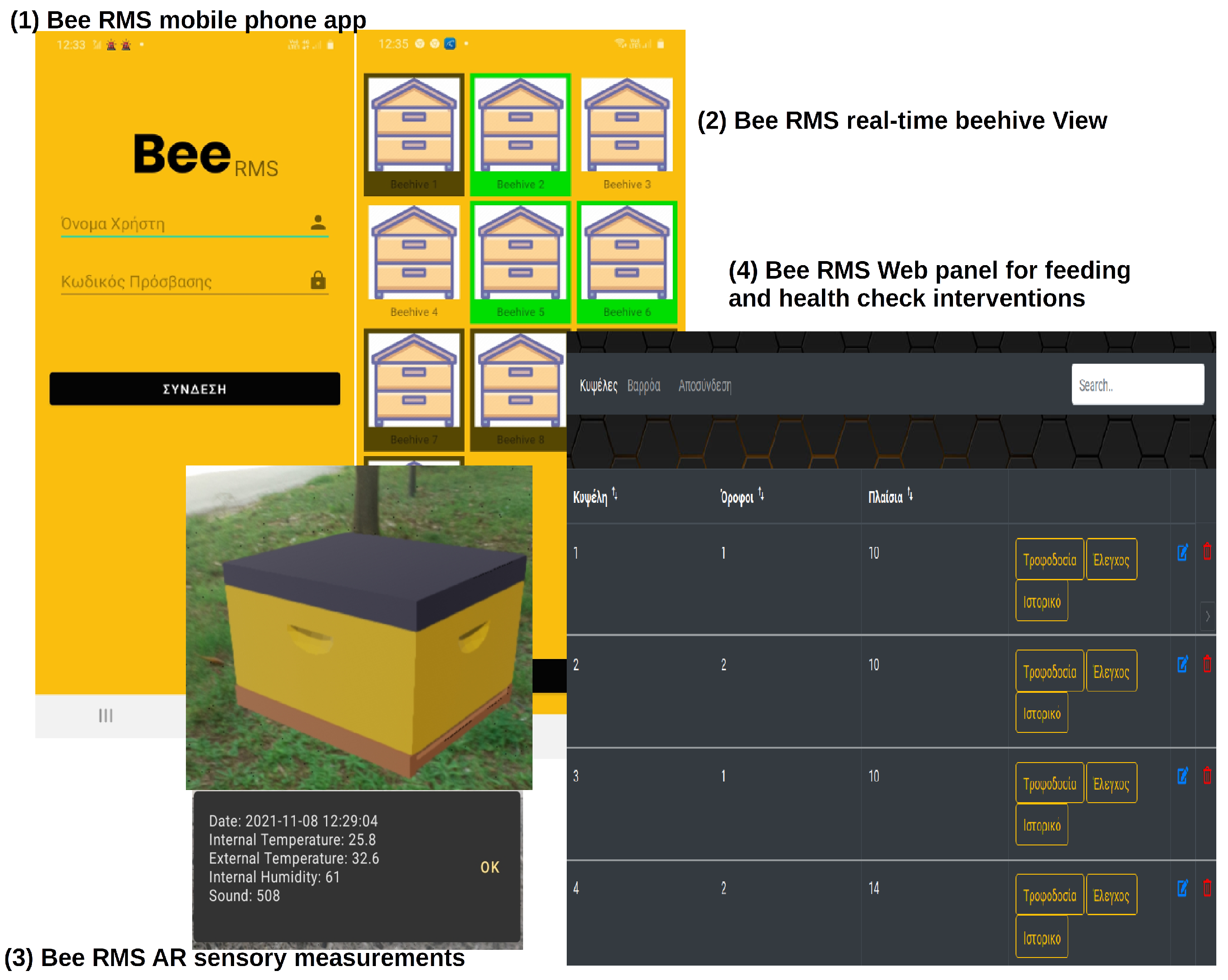
3.3. Beehive Quality Resource Management System

The BeeQ RMS system is a SaaS cloud service capable of interacting with the end nodes via the concentrator and the end-users. For Version 1 devices, the end nodes periodically deliver images to the BeeQ RMS using HTTP put requests (Figure 1 P1). Then, the uploaded photos are processed at the RMS end using the motion detection and CNN algorithm and web interface (see Figure A5) of the BeeQ RMS swarming service (Figure 1 P2).

For Version 2 devices, the motion detection and CNN bee detection algorithm are performed directly at the end node. When the detection period is reached and only when bee motion is detected, the trained CNN engine is loaded, and the number of bees is calculated, as well as the severity of the event. The interdetection interval is usually statically set to 1–2 h. However, for Version 2 devices, the detection outcome is transmitted over the LoRaWAN network. It is collected and AES-128 decrypted by the BeeQ RMS LoRa application server, sending the detection message over MQTT via the BeeQ RMS MQTT broker. The BeeQ RMS MQTT then stores the message in the DB service, where the MQTT message is JSON decoded and stored in the BeeQ RMS MySQL database (see Figure 2, P1 and P2) [4]. Similarly, for Version 1 devices, the images are processed by the BeeQ RMS Swarm detection service (Figure 1 P2), responsible for the swarm detection process and storing the detection result at the BeeQ RMS MySQL database.

For both cases (Version 1, Version 2), the output result (number of detected bees and severity of alert) is delivered to the end-users using push notifications. The Bee-RMS mobile phone application and dashboard are notified accordingly (Figure 1 P3 and Figure 2 P3). The Version 1 and Version 2 device prototypes are illustrated in Figure A6.

3.4. Beehive End Node Application

The end node applications used by the BeeQ RMS system are the Android mobile phone app and the web panel. Both applications share the same operational and functional characteristics, that is, recording feeds and periodic farming checks, sensory input feedback for temperature, sound level increase, or humidity-related incidents (sensors fragment and web panels), and swarm detection alerts via the proposed system camera module. In addition, the Firebase push notifications service is used [45], while for the web dashboard, the jQuery notify capabilities are exploited.

4. Deep-Learning System Training and Proposed Detection Process

In this section, the authors describe their utilized deep-learning detection process for bee swarming inside the beehive. The defined approach is a part of the pre-trained CNN models, and CNN algorithms [46,47], which after the use of motion-detection filtering, try to estimate if swarming conditions have been reached.

The process used to build and test the swarming operation for detecting bees includes four steps for the CNN-training process. Furthermore, the detection service also consists of three stages, as illustrated in Figure 3. The CNN training steps used are as follows:

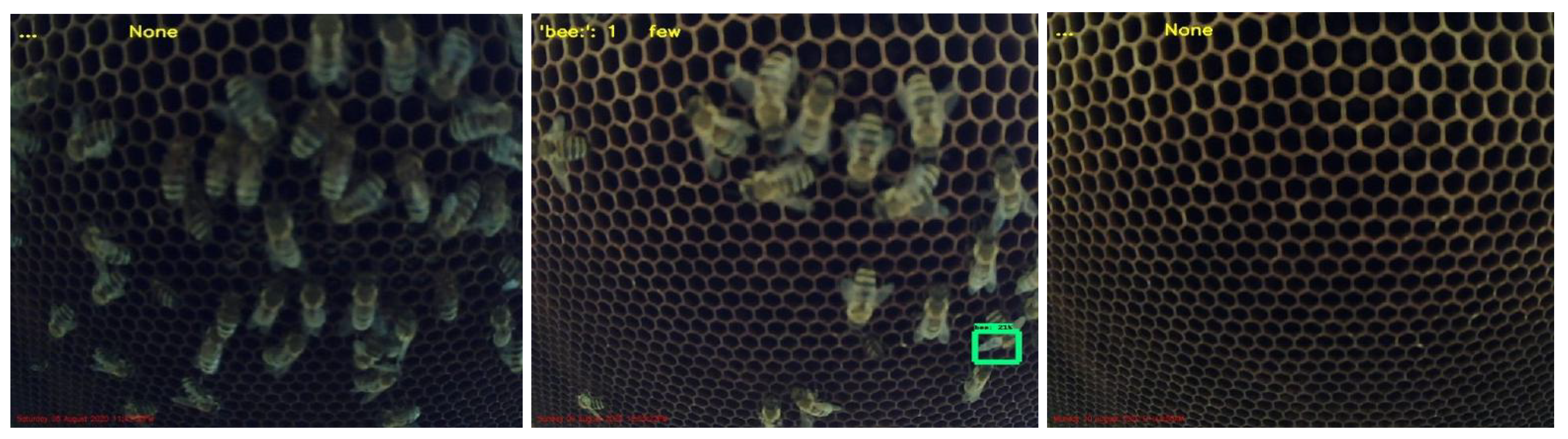
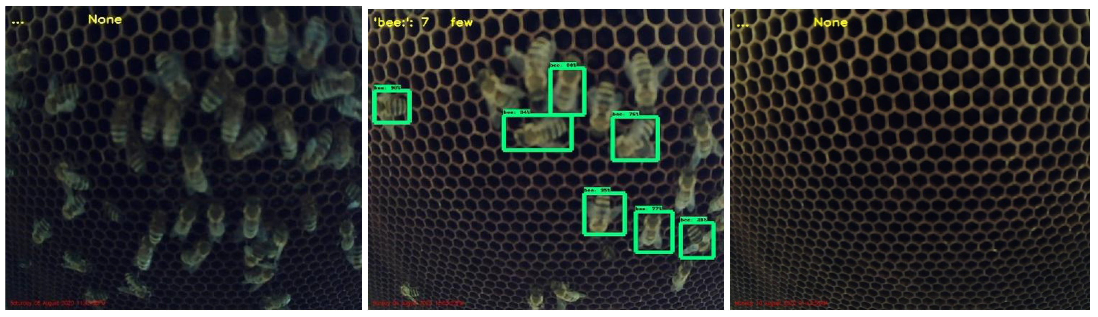
• Step 1—Initial data acquisition and data cleansing: The initial imagery dataset acquired by the beehive-monitoring module is manually analyzed and filtered to eliminate blurred images or images with a low resolution and light intensity. The photos in this experimentation taken from the camera module are set to a minimum acquisition of 0.5 Mpx in size of 800 × 600 px 300 dpi (67.7 × 50.8 mm${}^2$) compressed in the JPEG format using a compression ratio Q = 70 (22,91) of 200–250 KB each. That is because the authors wanted to experiment with the smallest possible size of image transmission (due to the per GB network provider costs of image transmissions for Version 1 devices or to minimize processing time overheads for Version 2 devices). Similarly, the trained CNN and algorithms used are the most processing-light for portable devices, using a minimum trained image size input of 640 ×640 px (lightly distorted at the image height) and using cubic interpolation.
  The trained Convolutional Neural Network (CNN) is used to solve the problem of swarming by counting the bee concentration above the bee frames and inside the beehive lid. The detection categories that the authors’ classifier uses are:
  Class 0: no bees detected;
  Class 1: a limited number of bees scattered on the frame or the lid (less than 10);
  Class 2: a small number of bees (less than or equal to 20);
  Class 3: initial swarm concentration and a medium number of bees concentrated (more than 20 and less than or equal to 50);
  Class 4: swarming incident (high number of bees) (more than 50).
  For each class, the number of detected bees was set as a class identifier (the class identifier boundaries can be arbitrarily set accordingly to the detection service configuration file). Therefore, the selected initial data-set may consist of at least 1000 images per detection class, a total of 5000 images used for training the CNN;
• Step 2—Image transformation and data annotation: The number of collected images per class used for training was annotated by hand using the LabelImg tool [48]. Other commonly used annotation tools are Labelbox [49], ImgAnnotation [50], and Computer Vision Annotation Tool [51], all of which provide an XML annotated output.
  Image clearness and resolution are equally important in the case of initially having different image dimensions. Regarding photo clearness, the method used is as follows. A bilateral filter smooths all images using a degree of smoothing sigma = 0.5–0.8 and a small 7 × 7 kernel. Afterward, all photos must be scaled to particular and fixed dimensions to be inserted into the training network. Scaling is performed either using a cubic interpolation process, or a super-resolution EDSR process [52]. The preparation of the images is based on the dimensions required as the input by the selected training algorithm, which matches with the underlying extent of the initial CNN layer. The image transformation processes were implemented using OpenCV [53] and were also part of the 2nd stage of the detection process (detection service) before their input into the CNN engine (see Figure 3);
• Step 3—Training process: The preparation of the training process is based on using pre-trained Convolution Neural Network (CNN) models [54,55], TensorFlow [56] (Version 1), and the use of all available CPU and GPU system resources. To achieve training parallel execution speed up, the use of a GPU is necessary, as well as the installation of the CUDA toolkit such that the training process utilizes the GPU resources, according to the TensorFlow requirements [57].
  The CNN model’s design includes selecting one of the existing pre-trained TensorFlow models, where our swarming classifier will be included as the final classification step. Selected core models for TensorFlow used for training our swarming model and their capabilities are presented in

  Table 2. CNN models used during the training step.

  CNN Mode [54,55]	CNN Models Capabilities
  	Input Images Size (wxh) (px)	Model Classes	Models Mean Detection Time per (ms)	Model Accuracy mAP
  SSD - MobileNet v1	300 × 300	90	30	21
  SSD - MobileNet v2	300 × 300	90	31	22
  SSD - Inception v2	300 × 300	90	42	24
  Faster-RCNN - Inception v2	600–1024 × 600–1024	90	58	28

  . Once the Step 2 annotation process is complete and the pre-trained CNN model is selected, the images are randomly divided into two sets. The training set consisted of 80% of the annotated images, and the testing set contained the remaining 20%. The validation set was also used by randomly taking 20% of the training set;
• Step 4—Detection service process: This process is performed by a detection application installed as a service that loads the CNN inference graph in memory and processes arbitrary images received via HTTP put requests from the node Version 1 device. The HTTP put method requires that the requested URI be updated or created to be enclosed in the put message body. Thus, if a resource exists at that URI, the message body should be considered as a new modified version of that resource. If the put request is received, the service initiates the detection process and, from the detection JSON output for that resource, creates a new resource XML response record. Due to the asynchronous nature of the swarming service, the request is also recorded into the BeeQ RMS database to be accessible by the BeeQ RMS web panel and mobile phone application. Moreover, the JSON output response, when generated, is also pushed to the Firebase service to be sent as push notifications to the BeeQ RMS mobile phone application [45,58]. Figure 3 analytically illustrates the detection process steps for both Version 1 and Version 2 end nodes.
  Step 1 is the threshold max-contour image selection process issued only by Version 2 devices as part of the sequential frames’ motion detection process instantiated periodically. Upon motion detection, photo frames that include the activity notification contours for Version 2 devices or uploaded frames from Version 1 devices are transformed through a bilateral filtering transformation with sigma_space and sigma_color parameters equal to 0.75 and a pixel neighborhood of 5 px. Upon bilateral filter smoothing, the scaling process initiates to normalize images to the input dimensions of the CNN. For down-scaling or minimum dimension up-scaling (up to 100 px), cubic interpolation is used, while for large up-scales, the OpenCV super-resolution process is instantiated (Enhanced Deep Residual Networks for Single Image Super-Resolution) [52] using the end node device. Upon CNN image normalization, the photos are fed to the convolutional neural network classifier, which detects the number of bee contours and reports it using XML output image reports, as presented below:
  <detection>
  <bees>Number of bees</bees>
  <varroa>
  <detected>True/False</detected>
  <num>Number of bees</num>
  </varroa>
  <queen>
  <detected>True/False</detected>
  </queen>
  <hornets>
  <detected>True/False</detected>
  <num>Number of hornets</num>
  </hornets>
  <notes>
  Instructions for dealing with diseases.
  </notes>
  </detection>
  Apart from bee counting information, the XML image reports also include the information of detected bees carrying the Varroa mite. Such detection can be performed using two RGB color masks over the detected bee contours. This functionality is still under validation and therefore set as future work and exploitation of the CNN bee counting classifier. Nevertheless, this capability was included in the web interface but not thoroughly tested. Similarly, the automated queen detection functionality (now performed using the check status form report in the Bee RMS web application) was also included as a capability of the web detection interface. The Bee RMS classifier is still under data collection and training since the preliminary trained models used a limited number of images. The algorithmic process includes a new detection queen bee class and the HSV processing of the bee queen’s color to estimate its age.
  Upon generation of the XML image report, the swarming service loads the report and stores it in the BeeQ RMS database to be accessible by the web BeeQ RMS interface and transforms it to a JSON object to be sent to the Firebase service [45,58]. The BeeQ RMS Android mobile application can receive such push notifications and appropriately notify the beekeeper.

The following section presents the authors’ experimentation using different trained neural networks and end node devices.

5. Experimental Scenarios

In this section, the authors present their experimental scenarios using Version 1 and Version 2 end node devices and their experimental results while detecting bees using the two selected CNN algorithms (SSD and Faster-RCNN) and two selected models: MobileNet v1 and Inception v2. These models were chosen from a set of pre-trained models based on their low mean detection time and good mean Average Precision (mAP) results (as illustrated in Table 2). Two different CNN algorithms were used during experimentation; SSD and Faster R-CNN. Using the SSD algorithm, two different pre-trained models have been utilized: The MobileNet v1 and Inception v2 COCO models. For the Faster R-CNN algorithm the Inception v2 model has been used.

For the CNN training process, the total number of images in the data-set annotated and used for the models’ training in this scenario was 6627 with dimensions of 800×600 px. One hundred of them were randomly selected for the detection validation process. The constructed network was trained to detect bee classes, as described in the previous section. The Intersection over Union (IoU) threshold was set to 0.5.

During the training processes, the TensorBoard has been used. The TensorBoard presents and records the loss charts during training. The values shown in the loss diagrams are the values obtained from the loss functions of each algorithm [59]. Looking at the recorded loss charts, it is evident whether the model would have a high degree of accuracy in detection. For example, if the last calculated loss is close to zero, it is expected for the model to have a high degree of accuracy. In contrast, the further away from zero, the more the accuracy of the model decreases. After completing the training of the three trained networks, the initial and final loss training values and the total training time are presented in

Table 3. CNN trained models’ loss values and total training time.

CNN Models	Initial Loss Value	Final Loss Value	Total Training Time
SSD - MobileNet v1	11.90	0.7025	35 h 47 min
SSD - Inception v2	4.095	0.8837	43 h 15 min
Faster-RCNN - Inception v2	1.438	0.0047	14 h 27 min

.

The authors performed their validation detection tests using 100 beehive photos. For each test, five different metrics were measured: the time required to load the trained network into the system memory, the total detection time, the average ROI detection time, the mean Average Precision (mAP) derived from the models’ testing for IoU = 0.5, and the maximum memory allocation per neural network.

Furthermore, the detection accuracy (DA) and the mean detection accuracy (MDA) were also defined by the authors. That is, by performing manual bee counting for each detected bee contour with a confidence level threshold above 0.2 over the total images. The detection accuracy (DA) and the mean detection accuracy (MDA) metrics are calculated using the Equation (1):

$$DA=\frac{DC}{N},MDA=\frac{1}{M}\sum _{i=1}^{M}D{A}_i$$

(1)

where variable $DC$ is the contours that have been marked and have bees, the variable N is the total number of bees in the photo, while the variable M is the number of photos we tested. The following error metric (Er) was also defined, which occurs during the detection process, using the Equation (2):

$$Er=1-\frac{DC}{C}$$

(2)

where variable C is the total number of contours marked by the model. The accuracy of the object detection was also measured by the mAP using TensorBoard. That is, the average of the maximum precisions at different detected contours over the real annotated ones. Precision measures the prediction accuracy by comparing the true positives and all the false-negative cases.

The tests have been performed on three different CPU Version 2 devices and in the cloud by utilizing either a single-core cloud CPU or a 24-core cloud CPU for testing Version 1 end node devices’ cloud processing requirements. The memory capabilities for the single-core cloud CPU were 8 GB, while for the 24-core cloud CPU, 64 GB. For the Version 2 tested devices, the authors utilized a Raspberry Pi-3 armv7 1.2 GHz quad-core with 1 GB of RAM and a 2 GB swap, and a Raspberry Pi zero armv6 1GHz single-core, 512 MB RAM, and 2 GB swap. Both RPi nodes’ OS was the 32 bit Raspbian GNU/Linux operating system. A third Version 2 end node device was also tested the NVIDIA Jetson Nano board. Jetson has a 1.4 GHz quad-core armv7 processor, 128-core NVIDIA Maxwell GPU, and its memory capacity is 4 GB, used either by the CPU or GPU. The Jetson operating system is a 32 bit Linux for Tegra.

5.1. Scenario I: End Node Version 1 Detection Systems’ Performance Tests

Scenario I detection tests included Version 1 end node device-equipped systems’ performance test using cloud (a) single-core and (b) multi-core CPUs and Version 1 end node devices. During these tests for the (a) and (b) system cases, the two selected algorithms (SSD, Faster-RCNN) and their trained models were tested for their performance. The results for Cases (a) and (b) are presented in

Table 4. Experimental Scenario I, x64 CPU CNN detection time and memory usage.

CNN Models	Load Time (s)	Testing Detection Time (s)	Detection Average Time per Image (s)	Total Time (s)	Memory Usage (MB)
SSD - MobileNet v1	0.291	1.340	0.105	1.631	45.262
SSD - Inception v2	0.432	1.523	0.156	1.955	106.889
Faster-RCNN - Inception v2	0.368	5.358	1.079	5.726	104.327

and

Table 5. Experimental Scenario I, x64, 24-core CPU detection time and memory usage.

CNN Models	Load Time (s)	Testing Detection Time (s)	Detection Average Time per Image (s)	Total Time (s)	Memory Usage (MB)
SSD - MobileNet v1	0.309	1.335	0.087	1.644	45.262
SSD - Inception v2	0.431	1.361	0.109	1.792	106.889
Faster-RCNN - Inception v2	0.386	2.249	0.278	2.635	104.327

accordingly.

Based on Scenario I’s result for single-core x86 64-bit CPUs, using the SSD on the MobileNet v1 network provided the best TensorFlow network load time (32% less than the SSD Inception model and 15% less than the Faster-RCNN Inception model). Comparing the load times of the Inception models for the SSD and Faster-RCNN algorithms showed that Faster-RCNN provided an optimum faster loading model than its SSD counterpart. Nevertheless, the SSD single-image average detection time was 2.5-times faster than its Faster-RCNN counterpart. Similar results were applied and for SSD-MobileNet v1 (three times faster).

Comparing Table 3 and Table 4, it is evident that Faster-RCNN Inception v2 had the minimum total loss value (0.0047%), as indicated by the training process and the least training time, while the SSD algorithms showed high loss values of 0.7% and 0.8% accordingly. Having as the performance indicator metric the Mean Detection Accuracy (MDA), provided in Table 7, over the total detection time per image, the authors defined a CNN evaluation metric called the Success Frequency (S.F.) metric, expressed by Equation (3). However, if it is not possible to validate the model using the MDA metric, the model mAP accuracy values can be used instead (see Equation (4)).

$$SF=\frac{MDA}{T_{load}+T_{detect}}$$

(3)

$$S{F}_{mAP}=\frac{mAP}{T_{load}+T_{detect}}$$

(4)

where T${}_{load}$ is the mean frame load time (s) and T${}_{detect}$ is the mean CNN frame detection time (s). The S.F. metric expresses the number of ROIs (contours) per second successfully detected over time. The S.F. values over the mAP and image detection times are depicted in Figure 4. The S.F. metric is critical for embedded and low-power devices with limited processing capabilities (studied in Scenario II). Therefore, it is more suitable for the CNN algorithm to be selected based on the highest S.F. value instead of the CNN mAP or total loss for such devices.

Comparing the single x86 64bit CPU measurements with the 24-CPU measurements (Table 4 and Table 5), the speedup value $\sigma$ can be calculated using the mean detection time as $\sigma =\frac{T_1}{T_{24}}$ since the mean CNN detection time is a parallel task among the 24 cores. Therefore, the speedup achieved using 24 cores for the SSD algorithm was almost constant, close to $\sigma =1.1$. Therefore, with the SSD algorithm for cloud 24-core CPUs, using a single-core provided the same results in terms of performance. However, for the Faster-RCNN, using 24 cores offered a double performance speedup of $\sigma =2.3$, that is to reduce the per-image detection time, 50%, at least 24 cores would need to operate in parallel, contributing to the detection process of Faster-RCNN.

5.2. Scenario II: End Node Version 2 Detection Systems’ Performance Tests

Scenario II detection tests included Version 2 devices’ performance tests as standalone devices (no cloud support). The end node systems that were tested were: (a) single-core ARMv6, (b) quad-core ARMv7, and (c) CPU+GPU quad-core ARMv7 Jetson device. During these tests, the two selected algorithms (SSD, Faster-RCNN) and their trained models were tested in terms of performance. The performance results are presented in

Table 6. Experimental Scenario II, RPi ARMv7, ARMv6 single-core and Jetson Nano CPU ARMv7 + GPU performance comparison results.

	Load Time (s)	Mean CNN Time (s)	Mean ROI Time (s)	Total Time (s)	MeM Usage (MB)	S.F. mAP
CNN Models	ARM single-core ――――-	ARM single-core ――――-	ARM single-core ――――-	ARM single-core ――――-	ARM single-core ――――-	ARM single-core ――――-
	ARM quad-core ――――-	ARM quad-core ――――-	ARM quad-core ――――-	ARM quad-core ――――-	ARM quad-core ――――-	ARM quad-core ――――-
	ARM quad-core + GPU	ARM quad-core + GPU	ARM quad-core + GPU	ARM quad-core + GPU	ARM quad-core + GPU	ARM quad-cor + GPU
SSD - MobileNet v1	10.97 ――――-	29.297 ――――-	2.955 ――――-	40.267 ――――-	75.924 ――――-	0.01 ――――-
	10.597 ――――-	22.561 ――――-	2.457 ――――-	33.158 ――――-	75.924 ――――-	0.012 ――――-
	7.916	33.524	6.606	41.44	81.02	0.01
SSD - Inception v2	15.381 ――――-	34.884 ――――-	6.614 ――――-	50.265 ――――-	174.449 ――――-	0.008 ――――-
	15.318 ――――-	36.072 ――――-	6.886 ――――-	51.39 ――――-	174.449 ――――-	0.0079 ――――-
	10.614	61.106	13.416	71.72	181.08	0.0056
Faster-RCNN - Inception v2	14.389 ――――-	184.373 ――――-	41.826 ――――-	198.762 ――――-	166.351 ――――-	0.003 ――――-
	14.243 ――――-	111.333 ――――-	24.222 ――――-	125.576 ――――-	166.351 ――――-	0.0058 ――――-
	9.957	69.968	15.5	79.926	172.729	0.009

.

As shown in Table 6, the S.F. mAP values for the embedded micro-devices indicated that the best algorithm to use was the SSD with the MobileNet v1 network. This algorithm had similar S.F. value results for single-core ARM, quad-core, and Jetson devices. For less accurate detection networks of mAP values less than 0.5, there were no significant gains from using multi-core embedded systems.

This was not the case for high-accuracy detection devices, which can provide mAP values of more than 0.7, such as the Faster-RCNN. In these cases, the use of multiple CPUs and GPUs can offer significant gains of 40–50%, in terms of S.F. (both detection time reduction and accuracy increase as signified by the mAP). Since energy requirements for the devices are critical, for low-energy devices, the SSD MobileNet v1 is preferred using an ARMv6 single-core CPU (since the S.F. increase of ARMv6 concerning the use of four cores to achieve such a result was considered by the authors to be a significant energy expenditure).

For high-accuracy devices, the Jetson board using the Faster-RCNN algorithm provided the best results in terms of accuracy and execution time. Performance tests on the Jetson Nano microcomputer showed that the results obtained from this system for high accuracy were better than the ones from the RPi 3, due to the GPU’s participation in the detection process. However, in the Jetson Nano microprocessor, some transient errors occurred during the CPU and GPU allocation, which did not cause significant problems during the detection process. Nevertheless, since no energy measurements were performed for the quad-core RPi and Jetson, the RPi can also be considered a low-energy, high-accuracy alternative instead of the Jetson Nano, according to the devices’ data-sheets.

5.3. Scenario III: CNN Algorithms’ and Models’ Accuracy

Scenario III’s detection tests focused on the accuracy of the two used algorithms and their produced trained CNNs, using the mean detection accuracy metric from Equation (1) and the mAP values calculated by the TensorBoard during the training process. The results are presented in

Table 7. Mean detection accuracy (manual bee counting verification) over models’ mAP.

CNN Models	Mean Detection Accuracy (MDA)	CNN Model mAP	x86-64 Single-Core CPU SF	ARM Single-Core CPU SF
SSD - MobileNet v1	0.418	0.4223	0.009	0.01
SSD - Inception v2	0.13	0.4083	0.001	0.002
Faster-RCNN - Inception v2	0.703	0.7308	0.006	0.003

. Furthermore, the detection image results are illustrated in Figure A1, Figure A2 and Figure A3 in Appendix A, using the Jetson Nano Version 2 device and the SSD and Faster-RCNN algorithms on their trained models.

According to the models’ accuracy tests, the following conclusions were derived. First, based on the training process (Table 3), the Faster-RCNN algorithm with the Inception v2 model was faster to train than SSD. In addition, based on Table 3 and Table 7, the authors concluded that the lower the values of the training losses, the better the results we would obtain during the detection. It is also apparent that the best model for Version 2 devices with limited resources is SSD-MobileNet v1, as also shown in Table 7, by the S.F. values. That is because it requires less memory and processing time to work; regardless, it was 30% less accurate than the Faster-RCNN algorithm in terms of the MDA metric.

5.4. Scenario IV: System Validation for Swarming

The proposed swarming detection system was validated for swarming in two distinct cases:

Case 1—Overpopulated beehive. In this test case, a small beehive of five frames was used and monitored for a period of two months (April 2021–May 2021), using the Version 1 device. The camera module was placed (see Figure A6A, end node Version 1), facing the last empty beehive frame. The system successfully managed to capture the population increase (see Figure A5), reaching from the detection of Class-1 to a Class-3 initial swarm concentration and a medium number of bees concentrated. As a provocative measure, a new frame was added.

Case 2—Provoked swarming. In this test case, in a beehive colony during the early spring periodic check (March 2021), a new bee queen cell was detected by the apiarists, indicating the incubation of a new queen. The Version 1 device with the camera module was placed facing the area above the frames, towards the ventilation holes. Between the frames and the lid, the beehive’s progress was monitored weekly (weekly apiary checks). In the first two weeks, a significant increase of bee clustering was monitored, varying from the detection of Class-1 to Class-3 and back to Class-0. The apiarists also matched the swarming indication to the imminent swarming event since a significant portion of the hive population had abandoned the beehive.

In the above-mentioned cases, Case-1 experiments were successfully performed more than once. Both validation test cases were performed at our laboratory beehive station located in Ligopsa, Epirus, Greece, and are mentioned in this section as proof of the authors’ proposed concept. Nevertheless, more extensive validation and evaluation are set as future work.

6. Conclusions

This paper presented a new beekeeping-condition-monitoring system for the detection of bee swarming. The proposed system included two different versions of the end node devices and a new algorithm that utilizes CNN deep-learning networks. The proposed algorithm can be incorporated either at the cloud or at the end node devices by modifying the system’s architecture accordingly.

Based on their system end-node implementations, the authors’ experimentation focused on using different CNN algorithms and end node embedded modules. The authors also proposed two new metrics, the mean detection accuracy, and success frequency. These metrics were used to verify the mAP and total loss measurements and to make a trade-off between detection accuracy and limited resources due to the low energy consumption requirements of the end node devices.

The authors’ experimentation made it clear that low-processing mobile devices can use less accurate CNN detection algorithms. Instead, metrics can be used that can accurately represent each CNN’s resource utilization, such as S.F., MDA, and speedup ($\sigma$), for the acquisition of either the appropriate embedded device configuration or cloud resource utilization. Furthermore, appropriate validation of the authors’ proposed system was performed in two separate cases of (a) bee queen removal and (b) a beehive population increase that may lead to a swarming incident if not properly ameliorated with the addition of frames in the beehive.

The authors set at future work the extensive evaluation of their proposed system towards swarming events and the extension of their experimentation towards other deep-learning CNN algorithms. Furthermore, the authors set as future work energy consumption of the Version 1 and 2 devices.

References

1. Abbasi, M.; Yaghmaee, M.H.; Rahnama, F. Internet of Things in agriculture: A survey. In Proceedings of the 2019 3rd International Conference on Internet of Things and Applications (IoT), Heraklion, Greece, 2–4 May 2019; Volume 1, pp. 1–12. [Google Scholar] [CrossRef]
2. Farooq, M.S.; Riaz, S.; Abid, A.; Abid, K.; Naeem, M.A. A Survey on the Role of IoT in Agriculture for the Implementation of Smart Farming. IEEE Access 2019, 7, 156237–156271. [Google Scholar] [CrossRef]
3. Farooq, M.S.; Riaz, S.; Abid, A.; Umer, T.; Zikria, Y.B. Role of IoT Technology in Agriculture: A Systematic Literature Review. Electronics 2020, 9, 319. [Google Scholar] [CrossRef] [Green Version]
4. Zinas, N.; Kontogiannis, S.; Kokkonis, G.; Valsamidis, S.; Kazanidis, I. Proposed Open Source Architecture for Long Range Monitoring. The Case Study of Cattle Tracking at Pogoniani. In Proceedings of the 21st Pan-Hellenic Conference on Informatics; ACM: New York, NY, USA, 2017. [Google Scholar] [CrossRef]
5. Kontogiannis, S. An Internet of Things-Based Low-Power Integrated Beekeeping Safety and Conditions Monitoring System. Inventions 2019, 4, 52. [Google Scholar] [CrossRef] [Green Version]
6. Mekala, M.S.; Viswanathan, P. A Survey: Smart agriculture IoT with cloud computing. In Proceedings of the 2017 International conference on Microelectronic Devices, Circuits and Systems (ICMDCS), Vellore, India, 10–12 August 2017; Volume 1, pp. 1–7. [Google Scholar] [CrossRef]
7. Zabasta, A.; Kunicina, N.; Kondratjevs, K.; Ribickis, L. IoT Approach Application for Development of Autonomous Beekeeping System. In Proceedings of the 2019 International Conference in Engineering Applications (ICEA), Azores, Portugal, 8–11 July 2019; Volume 1, pp. 1–6. [Google Scholar] [CrossRef]
8. Flores, J.M.; Gamiz, V.; Jimenez-Marin, A.; Flores-Cortes, A.; Gil-Lebrero, S.; Garrido, J.J.; Hernando, M.D. Impact of Varroa destructor and associated pathologies on the colony collapse disorder affecting honey bees. Res. Vet. Sci. 2021, 135, 85–95. [Google Scholar] [CrossRef] [PubMed]
9. Dineva, K.; Atanasova, T. ICT-Based Beekeeping Using IoT and Machine Learning. In Distributed Computer and Communication Networks; Springer International Publishing: Cham, Switzerland, 2018; pp. 132–143. [Google Scholar]
10. Olate-Olave, V.R.; Verde, M.; Vallejos, L.; Perez Raymonda, L.; Cortese, M.C.; Doorn, M. Bee Health and Productivity in Apis mellifera, a Consequence of Multiple Factors. Vet. Sci. 2021, 8, 76. [Google Scholar] [CrossRef] [PubMed]
11. Braga, A.R.; Gomes, D.G.; Rogers, R.; Hassler, E.E.; Freitas, B.M.; Cazier, J.A. A method for mining combined data from in-hive sensors, weather and apiary inspections to forecast the health status of honey bee colonies. Comput. Electr. Agric. 2020, 169, 105161. [Google Scholar] [CrossRef]
12. Jarimi, H.; Tapia-Brito, E.; Riffat, S. A Review on Thermoregulation Techniques in Honey Bees’ (Apis Mellifera) Beehive Microclimate and Its Similarities to the Heating and Cooling Management in Buildings. Future Cities Environ. 2020, 6, 7. [Google Scholar] [CrossRef]
13. Peters, J.M.; Peleg, O.; Mahadevan, L. Collective ventilation in honeybee nests. Future Cities Environ. 2019, 16, 20180561. [Google Scholar] [CrossRef] [Green Version]
14. Zacepins, A.; Kviesis, A.; Stalidzans, E.; Liepniece, M.; Meitalovs, J. Remote detection of the swarming of honey bee colonies by single-point temperature monitoring. Biosyst. Eng. 2016, 148, 76–80. [Google Scholar] [CrossRef]
15. Zacepins, A.; Kviesis, A.; Pecka, A.; Osadcuks, V. Development of Internet of Things concept for Precision Beekeeping. In Proceedings of the 18th International Carpathian Control Conference (ICCC), Sinaia, Romania, 28–31 May 2017; Volume 1, pp. 23–27. [Google Scholar] [CrossRef]
16. Gil-Lebrero, S.; Quiles-Latorre, F.J.; Ortiz-Lopez, M.; Sanchez-Ruiz, V.; Gamiz-Lopez, V.; Luna-Rodriguez, J.J. Honey Bee Colonies Remote Monitoring System. Sensors 2017, 17, 55. [Google Scholar] [CrossRef] [Green Version]
17. Bellos, C.V.; Fyraridis, A.; Stergios, G.S.; Stefanou, K.A.; Kontogiannis, S. A Quality and disease control system for beekeeping. In Proceedings of the 2021 6th South-East Europe Design Automation, Computer Engineering, Computer Networks and Social Media Conference (SEEDA-CECNSM), Preveza, Greece, 24–26 September 2021; pp. 1–4. [Google Scholar] [CrossRef]
18. Ntawuzumunsi, E.; Kumaran, S.; Sibomana, L. Self-Powered Smart Beehive Monitoring and Control System (SBMaCS). Sensors 2021, 21, 3522. [Google Scholar] [CrossRef]
19. Prost, P.J.; Medori, P. Apiculture, 6th ed.; Intercept Ltd.: Oxford, UK, 1994. [Google Scholar]
20. Nikolaidis, I.N. Beekeeping Modern Methods of Intensive Exploitation, 11th ed.; Stamoulis Publications: Athens, Greece, 2005. (In Greek) [Google Scholar]
21. Clement, H. Le Traite Rustica de L’apiculture; Psichalos Publications: Athens, Greece, 2017. [Google Scholar]
22. He, W.; Zhang, S.; Hu, Z.; Zhang, J.; Liu, X.; Yu, C.; Yu, H. Field experimental study on a novel beehive integrated with solar thermal/photovoltaic system. Sol. Energy 2020, 201, 682–692. [Google Scholar] [CrossRef]
23. Kady, C.; Chedid, A.M.; Kortbawi, I.; Yaacoub, C.; Akl, A.; Daclin, N.; Trousset, F.; Pfister, F.; Zacharewicz, G. IoT-Driven Workflows for Risk Management and Control of Beehives. Diversity 2021, 13, 296. [Google Scholar] [CrossRef]
24. Terenzi, A.; Cecchi, S.; Spinsante, S. On the Importance of the Sound Emitted by Honey Bee Hives. Vet. Sci. 2020, 7, 168. [Google Scholar] [CrossRef] [PubMed]
25. Ferrari, S.; Silva, M.; Guarino, M.; Berckmans, D. Monitoring of swarming sounds in beehives for early detection of the swarming period. Comput. Electron. Agric. 2008, 64, 72–77. [Google Scholar] [CrossRef]
26. Nolasco, I.; Terenzi, A.; Cecchi, S.; Orcioni, S.; Bear, H.L.; Benetos, E. Audio-based Identification of Beehive States. In Proceedings of the IEEE International Conference on Acoustics, Speech and Signal Processing (ICASSP), Brighton, UK, 12–17 May 2019; Volume 1, pp. 8256–8260. [Google Scholar] [CrossRef] [Green Version]
27. Zgank, A. Bee Swarm Activity Acoustic Classification for an IoT-Based Farm Service. Sensors 2020, 20, 21. [Google Scholar] [CrossRef] [Green Version]
28. Nolasco, I.; Benetos, E. To bee or not to bee: Investigating machine learning approaches for beehive sound recognition. CoRR 2018. Available online: http://xxx.lanl.gov/abs/1811.06016 (accessed on 14 April 2019).
29. Liew, L.H.; Lee, B.Y.; Chan, M. Cell detection for bee comb images using Circular Hough Transformation. In Proceedings of the 2010 International Conference on Science and Social Research (CSSR 2010), Kuala Lumpur, Malaysia, 5–7 December 2010; pp. 191–195. [Google Scholar] [CrossRef]
30. Baptiste, M.; Ekszterowicz, G.; Laurent, J.; Rival, M.; Pfister, F. Bee Hive Traffic Monitoring by Tracking Bee Flight Paths. 2018. Available online: https://hal.archives-ouvertes.fr/hal-01940300/document (accessed on 5 September 2019).
31. Simic, M.; Starcevic, V.; Kezić, N.; Babic, Z. Simple and Low-Cost Electronic System for Honey Bee Counting. In Proceedings of the 28th International Electrotechnical and Computer Science Conference, Ambato, Ecuador, 23–24 September 2019. [Google Scholar]
32. Bee-Shop Security Systems: Surveillance Camera for Bees. 2015. Available online: http://www.bee-shop.gr (accessed on 14 June 2020).
33. EyeSon Hives Honey Bee Health Monitor. | Keltronix. 2018. Available online: https://www.keltronixinc.com/ (accessed on 7 June 2018).
34. Theodoros Belogiannis. Zygi Beekeeping Scales with Monitoring Camera Module. 2018. Available online: https://zygi.gr/en (accessed on 10 March 2021).
35. Arnia Remote Hive Monitoring System. Better Knowledge for Bee Health. 2017. Available online: https://arnia.co.uk (accessed on 4 June 2018).
36. Hive-Tech 2 Crowd Monitoring System for Your Hives. 2019. Available online: https://www.3bee.com/en/crowd/ (accessed on 16 March 2019).
37. Hivemind System to Monitor Your Hives to Improve Honey Production. 2017. Available online: https://hivemind.nz/for/honey/ (accessed on 10 March 2021).
38. Hudson, T. Easy Bee Counter. 2018. Available online: https://www.instructables.com/Easy-Bee-Counter/ (accessed on 8 September 2020).
39. Hudson, T. Honey Bee Counter II. 2020. Available online: https://www.instructables.com/Honey-Bee-Counter-II/ (accessed on 8 September 2020).
40. Gomez, K.; Riggio, R.; Rasheed, T.; Granelli, F. Analysing the energy consumption behaviour of WiFi networks. In Proceedings of the 2011 IEEE Online Conference on Green Communications, Online Conference, Piscataway, NJ, USA, 26–29 September 2011; Volume 1, pp. 98–104. [Google Scholar] [CrossRef]
41. Nurgaliyev, M.; Saymbetov, A.; Yashchyshyn, Y.; Kuttybay, N.; Tukymbekov, D. Prediction of energy consumption for LoRa based wireless sensors network. Wirel. Netw. 2020, 26, 3507–3520. [Google Scholar] [CrossRef]
42. Lavric, A.; Valentin, P. Performance Evaluation of LoRaWAN Communication Scalability in Large-Scale Wireless Sensor Networks. Wirel. Commun. Mob. Comput. 2018, 2018, 6730719. [Google Scholar] [CrossRef] [Green Version]
43. Van den Abeele, F.; Haxhibeqiri, J.; Moerman, I.; Hoebeke, J. Scalability Analysis of Large-Scale LoRaWAN Networks in ns-3. IEEE Internet Things J. 2017, 4, 2186–2198. [Google Scholar] [CrossRef] [Green Version]
44. Haxhibeqiri, J.; De Poorter, E.; Moerman, I.; Hoebeke, J. A Survey of LoRaWAN for IoT: From Technology to Application. Sensors 2018, 18, 3995. [Google Scholar] [CrossRef] [Green Version]
45. Mokar, M.A.; Fageeri, S.O.; Fattoh, S.E. Using Firebase Cloud Messaging to Control Mobile Applications. In Proceedings of the International Conference on Computer, Control, Electrical, and Electronics Engineering (ICCCEEE), Khartoum, Sudan, 21–23 September 2019; pp. 1–5. [Google Scholar] [CrossRef]
46. Wang, W.; Yang, Y.; Wang, X.; Wang, W.; Li, J. Development of convolutional neural network and its application in image classification: A survey. Opt. Eng. 2019, 58, 1–19. [Google Scholar] [CrossRef] [Green Version]
47. Bharati, P.; Pramanik, A. Deep Learning Techniques-R-CNN to Mask R-CNN: A Survey. In Computational Intelligence in Pattern Recognition; Springer: Singapore, 2020; pp. 657–668. [Google Scholar]
48. Tzudalin, D. LabelImg Is a Graphical Image Annotation Tool and Label Object Bounding Boxes in Images. 2016. Available online: https://github.com/tzutalin/labelImg (accessed on 20 September 2019).
49. Labelbox. Labelbox: The Leading Training Data Platform for Data Labeling. Available online: https://labelbox.com (accessed on 2 June 2021).
50. Image Annotation Tool. Available online: https://github.com/alexklaeser/imgAnnotation (accessed on 2 June 2021).
51. Computer Vision Annotation Tool (CVAT). 2021. Available online: https://github.com/openvinotoolkit/cvat (accessed on 2 June 2021).
52. Lim, B.; Son, S.; Kim, H.; Nah, S.; Lee, K.M. Enhanced Deep Residual Networks for Single Image Super-Resolution. In Proceedings of the IEEE Conference on Computer Vision and Pattern Recognition (CVPR) Workshops, Honolulu, HI, USA, 21–26 July 2017; Volume 1, pp. 1132–1140. [Google Scholar] [CrossRef] [Green Version]
53. Bradski, G. The OpenCV Library. Dr. Dobb’s J. Softw. Tools 2000, 25, 120–123. [Google Scholar]
54. GitHub-Tensorflow/Models: Models and Examples Built with TensorFlow 1. Available online: https://github.com/tensorflow/models/tree/r1.12.0 (accessed on 15 September 2018).
55. GitHub-Tensorflow/Models: Models and Examples Built with TensorFlow 2. 2021. Available online: https://github.com/tensorflow/models (accessed on 12 November 2020).
56. Abadi, M.; Agarwal, A.; Barham, P.; Brevdo, E.; Chen, Z.; Citro, C.; Corrado, G.S.; Davis, A.; Dean, J.; Devin, M.; et al. TensorFlow: Large-Scale Machine Learning on Heterogeneous Systems. 2015. Available online: https://www.tensorflow.org/ (accessed on 20 September 2018).
57. TensorFlow GPU Support. 2017. Available online: https://www.tensorflow.org/install/gpu?hl=el (accessed on 15 September 2018).
58. Moroney, L. The Firebase Realtime Database. In The Definite Guide to Firebase; Apress: Berkeley, CA, USA, 2017; pp. 51–71. [Google Scholar] [CrossRef]
59. Huang, J.; Rathod, V.; Sun, C.; Zhu, M.; Korattikara, A.; Fathi, A.; Fischer, I.; Wojna, Z.; Song, Y.; Guadarrama, S.; et al. Speed and accuracy trade-offs for modern convolutional object detectors. arXiv 2017, arXiv:1611.10012. [Google Scholar]
Figure 1. Beehive monitoring end node Version 1 device that includes a WiFi transponder and the beehive-monitoring system logic using v1 end node devices.
Inventions 06 00087 g001
Figure 2. Beehive monitoring end node Version 2 device that includes a LoRaWAN transponder and beehive-monitoring system logic using v2 end node devices.
Inventions 06 00087 g002
Figure 3. Bee swarming service automated detection process.
Inventions 06 00087 g003
Figure 4. S.F. metric in ROIs/second over the mAP.
Inventions 06 00087 g004