3.1. Estimates of the Parameters and j of the Double Logistic Distribution
Consider the experimental results for the
parameter. Some values of the mathematical expectation
M estimates of the parameter
for the sample size
N = 6 are shown below (
Table 1).
Analysis of the results presented shows that the methods used give a biased estimate of the parameter
. However, the bias of the estimate
depends only on the sample size
N and does not depend on the parameters of the distribution law. Therefore, it can be easily eliminated by introducing a bias correction. The unbiased estimate (ub) of the parameter
is equal to:
where
is the bias coefficient of the estimate
, depending on the sample size
N.
The bias of the estimate depends both on the sample size N, and on the parameters of the distribution law. This circumstance does not allow obtaining an unbiased estimate of the parameter by the classical method.
In addition, it turned out that the minimum and maximum values of the estimate
for a given sample size
N are proportional to the mathematical expectation of this estimate and can be calculated by the formulas:
where
and
are the minimum and maximum values of the estimate
;
and are coefficients depending on the sample size N.
The efficiency of the estimates of the parameter
will be characterized by the value of the variance.
Table 2 shows some values of the variance of estimates of the parameter
for the sample
N = 6.
It is seen from
Table 2 that in all the above cases, the estimate
is more effective than the estimate
, since it has less variance. The calculation results showed that the ratio of the standard deviation of the estimate
to the mathematical expectation for a fixed sample size
N is a constant value:
The results are shown in
Table 1 and
Table 2 indicate the effectiveness of the estimate obtained by the maximum likelihood method. For a complete characteristic, we will find the distribution law of the estimate
. Since the number of realizations in the experiment is large enough, i.e., value
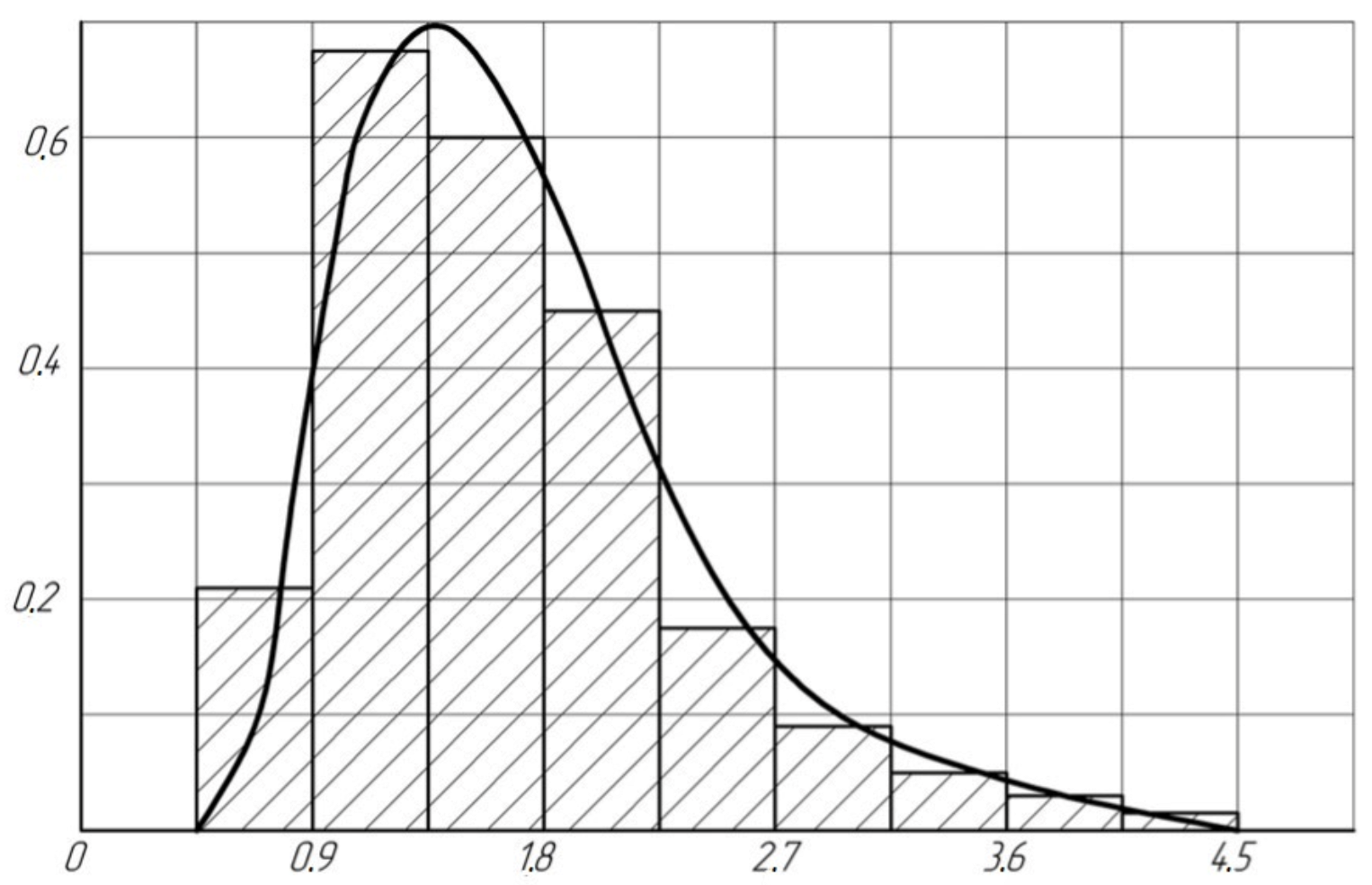
more, then it is advisable to use the histogram method. In
Figure 1, as an example, a histogram is shown for assessing
with a sample size
and the value of the parameters of the law under study
and
.
Analysis of the obtained histograms showed that the distribution of the estimate
with a sufficient degree of accuracy can be described by DLD with the parameters
,
,
and
. Parameters
and
are calculated by formulas (
5) and (
6) taking into account (
9), and the parameters
and
by formulas (
11) and (
12).
Taking into account that the DLD density function is reversible, for a given confidence probability
we can calculate interval estimates of the parameter
:
where
and
are the lower and upper bounds of the confidence interval of the estimate
.
To calculate the boundaries of the confidence interval of the estimate
, calculated from a small number of tests, the value of this estimate is substituted into formulas (
11), (
12) and (
14) instead of the mathematical expectation.
The values of the coefficients
,
,
and
, obtained experimentally, for all studied
N are given in
Table 3.
Studies have shown that to calculate the coefficients
,
,
and
, for any sample size
N you can use the following formulas:
The values , and are constants.
Let us consider the experimental results for the parameter
j.
Table 4 shows some values of the mathematical expectation of estimates of the parameter
j for a sample size of
N = 6.
Analysis of the results obtained shows that both methods used give a biased estimate of the parameter
j. Moreover, as for the parameter
, the bias of the estimate
depends only on the sample size
N and it can be taken into account by introducing a similar correction. Unbiased estimate of the parameter
j:
where
is the estimate bias coefficient
, depending on the sample size
N.
The bias of the estimate depends on the parameters of the distribution law and it is not possible to take it into account for this method.
The minimum
and maximum
estimates
can be calculated using the formulas:
The efficiency of estimates of the parameter
j, as well as for the parameter
, will be characterized by the value of the variance.
Table 5 shows some values of the variance of estimates of the parameter
j for the sample size
N = 6.
Table 5 shows that in all the cases considered, the
estimate is more effective than the
estimate, since it has a lower variance.
The variance of the
estimate for any sample size is calculated by the formula:
where
is a coefficient depending on the sample size
N.
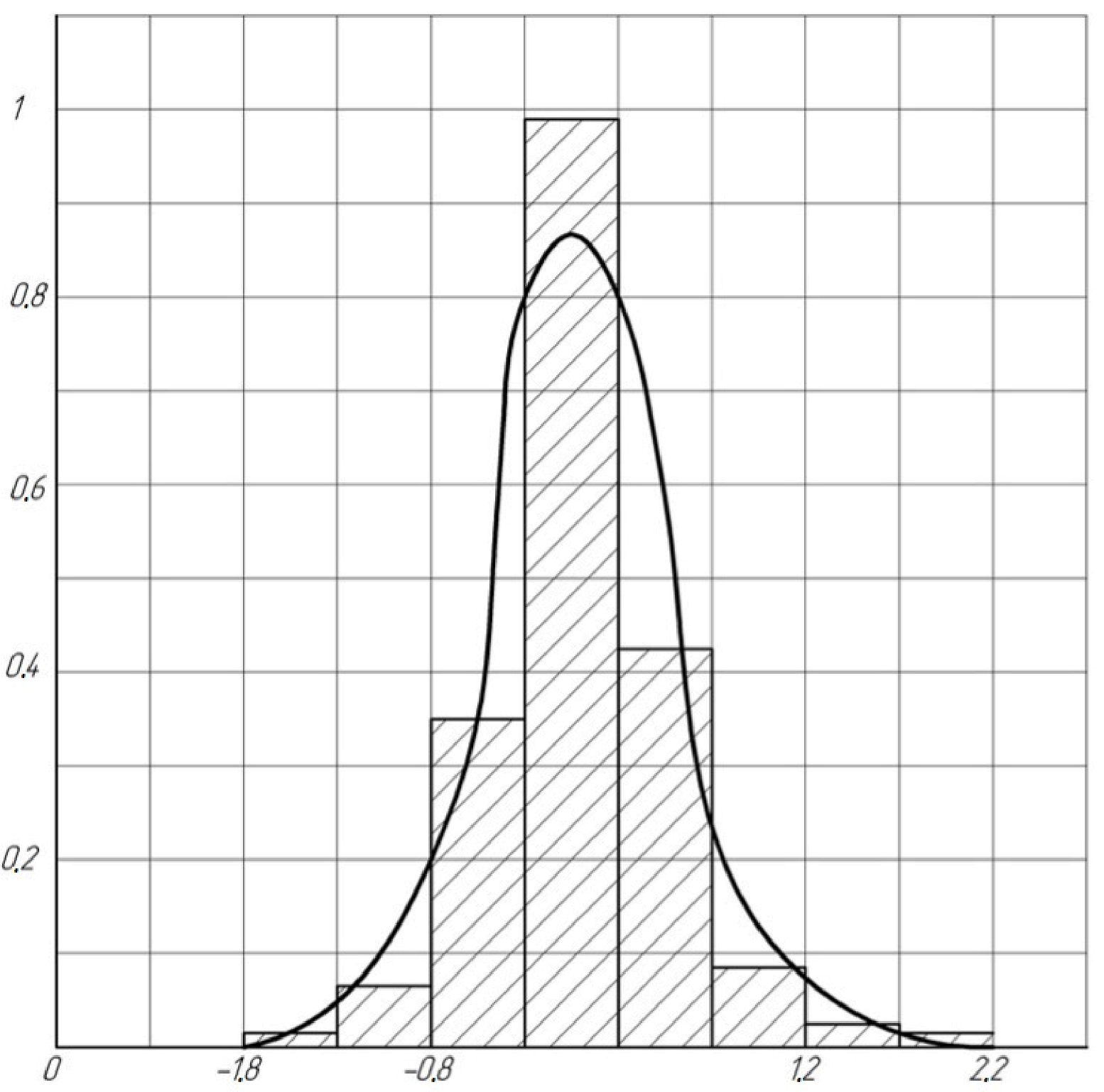
To fully characterize the estimate
we find the law of its distribution using the histogram method. In
Figure 2, as an example, a histogram is shown for evaluating
with a sample size
and the values of the parameters of the law under study
,
.
The analysis of the obtained histograms showed that the distribution of the
estimate with a sufficient degree of accuracy can be described by DLD with the parameters
,
,
and
. Parameters
and
are calculated by formulas (
5) and (
6) taking into account (
21) and (
24), and the parameters
and
by formulas (
22) and (
23). The numeric values
,
and
are constant.
Using the obtained distribution law of the estimate
, for a given confidence probability
we can calculate the interval estimates:
where
and
are, respectively, the lower and upper bounds of the confidence interval of the
estimate.
To calculate the boundaries of the confidence interval of the
calculated from a small number of tests, the value of this estimate is substituted into formulas (
22)–(
24) instead of the mathematical expectation.
The values of the coefficients
and
, obtained experimentally, for all studied
N, are given in
Table 6.
Studies have shown that the following formulas can be used to calculate the coefficients
and
for any sample size:
The numeric values , and are constant.
Thus, the analysis of the results of a statistical experiment for estimates and j of the selected distribution law allows us to draw the following conclusions:
The maximum likelihood method allows you to calculate unbiased estimates of the parameters and j, with minimum variance; the effectiveness of estimates and compared to estimates and , for example, with a sample size N = 6 and the parameters of the law under study and j = 0 are higher:
It was established by statistical modeling that the estimates and follow a double logistic distribution, therefore it is possible to calculate the exact confidence intervals for these parameters;
To calculate the point and interval estimates of the parameters and j, it is not required to draw up special tables.
3.2. Distribution Function Prediction
The parameters and calculated by the maximum likelihood method allow finding an estimate of the distribution function of a random variable x. For practical calculations with a small sample size, in addition, it is necessary to calculate the confidence zone of the distribution function. For this purpose, various well-known statistics can be used, for example, , (Mises), the maximum absolute divergence of the distribution functions . The selection of statistics is based on the following requirements:
It should be independent of the parameters of the adopted distribution law and be determined only by the sample size N;
the value of the statistics should not depend on any additional parameters, for example, on the number of intervals for dividing the domain of existence of the estimate;
Allowed calculating the confidence bounds of the distribution function [
9].
During the experiment, the three previously indicated statistics were investigated:, and . Analysis of the results of the experiment showed that the listed requirements are satisfied only by statistics calculated by the formula: .
Table 7, for example, shows some values of the mathematical expectation and variance of the statistics
with a sample size of
, as well as its largest value.
The above data confirm that the statistics
meet the requirements [
10].
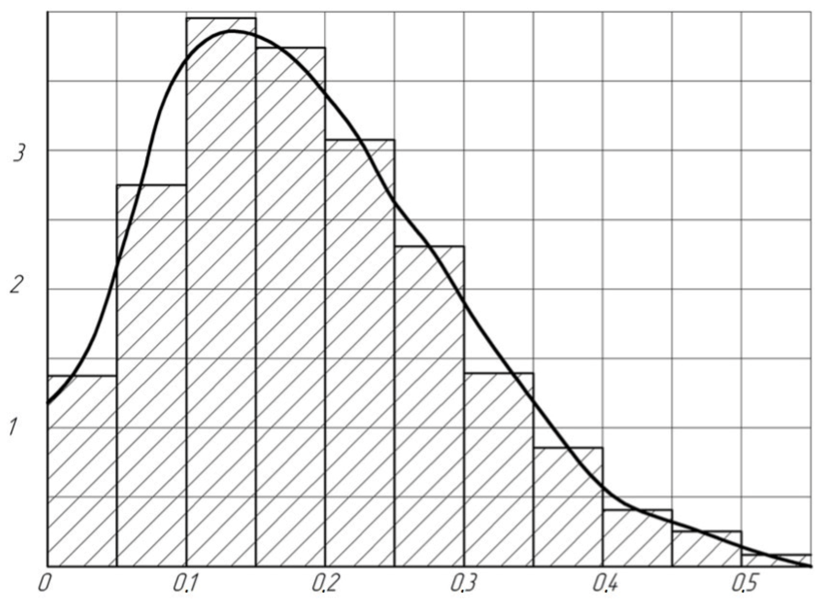
To fully characterize the statistics
let us find its distribution law using the histogram method. In
Figure 3 shows a histogram for statistics
with a sample size of
.
Studies have shown that the distribution of statistics
with a sufficient degree of accuracy can be described by DLD with the parameters
,
,
,
[
11,
12]. The parameters
and
are calculated by formulas (
5) and (
6). To calculate them, you need to know
and
.
Table 8 shows the values of
and
depending on the sample size.
Calculations have established that
,
and
for any sample size can be calculated by the formulas:
The values , and are constants.
Using the obtained distribution law of statistics
, interval estimates of the distribution function for a given confidence probability
, are calculated by the formulas:
where the value of the statistic
defined as follows:
The effectiveness of the proposed method for predicting the distribution law of a random variable
x will be estimated by the width of the confidence zone for the distribution function.
Table 9 shows the values of the statistics
for different confidence probabilities
and sample sizes.
The first lines of this table give the values
, calculated by (
34), the second lines—borrowed from [
13] and corresponding to the classical method of estimating the distribution law.
For comparison, let us calculate the required test volume
, which ensures the accuracy
. The same accuracy was obtained by the proposed method for a sample of
. To do this, we compose the equation:
solving which, we get:


 ,
, 


