

Continuum Logic of Control Signals in Analog Cyber–Physical Nets

Moscow Aviation Institute, Volokolamskoe Shosse 4, 125993 Moscow, Russia
Inventions 2023, 8(4), 101; https://doi.org/10.3390/inventions8040101
Submission received: 8 July 2023
/
Revised: 3 August 2023
/
Accepted: 9 August 2023
/
Published: 11 August 2023
(This article belongs to the Special Issue Recent Advances and New Trends in Signal Processing)
Abstract
:The use of embedded processors is the most promising direction in the development of automatic control systems. The article is devoted to analog models and technical solutions that allow continuous analysis of information in a technical system in order to synthesize control signals. Technical solutions are obtained on the basis of continuum logic methods, which aim to increase the speed of embedded computing networks, reduce power consumption, and unify the element base of analog processors. The effect of high speed is achieved due to the transition from sequential digital calculations to parallel synthesis of analog control signals. Examples of the implementation of schemes for the synthesis of control commands using the developed models of logical operations are given.
1. Introduction
Physiological processes occurring in living organisms obey the laws of continuous information exchange to ensure the integrity of the functioning of all organs in various conditions [1]. The parallelism of the formation of commands to the organs of a living organism and their consistency in order to achieve goals has been noted in the works of physiologists, starting with I.P. Pavlova. The current level of development of physiology confirms the thesis about the prospects for creating new technical solutions that replicate the diversity of living nature [2].
This paper proposes to consider the technical system TS as a distributed system, which differs from the well-known approach to the organization of computing structures [3] by using methods of continuous interaction of physical processors in executive bodies and analog devices. A network of embedded processors turns a technical system into a computing device that must meet such system requirements as cost, power consumption, and the use of limited physical resources [4].
The emergence of embedded real-time systems on microcontrollers has created conditions for the development of hybrid dynamic systems that demonstrate the characteristics of systems with both continuous and discrete time [5], can continuously change depending on differential inclusions, and can also change discretely in accordance with differential inclusions. The materials of the Cyber–Physical Systems seminar [6] were the first to formulate goals and objectives for the creation of a new systems science, which are both physical and computational, combining hardware and physical systems with software. Its appearance is associated with the theory of hybrid systems [7] and the algebra of synchronized processes [8].
Synchronization of the continuous and discrete time of change of variables is the main problem of hybrid systems. To determine whether the state function is true or not, the theory of temporal logic is applied [9]. The work [10] shows methods and means of combining the operation of analog and digital devices in embedded systems. However, their application does not solve the problem of compatibility of processes different in nature—physical and computational.
Problems do not arise when sufficiently slow robots [11] are designed, which are used in construction or driving a car. For fast applications, for example, for engine control, embedded systems are used [12], in which it is necessary to quickly and in real-time calculate nonlinear dependencies between parameters. A decrease in productivity is especially unacceptable when creating objects of microelectromechanical systems (MEMS) [2,13,14] and robotic complexes for military, special, and dual purposes [15]. The development of highly sensitive microsensors, spatial orientation devices, and micromechanical gearboxes [16,17,18] creates the prerequisites for the development of new methods for algorithmic control of miniature objects, in which the size and weight of computing devices can become a determining factor.
Object control systems that respond to changes in the parameters of the environment at the rate of receipt of messages from it belong to the class of reactive systems [19]. Their feature is an “instantaneous” reaction to changes in input signals. The development of reliable software for reactive systems requires the coordination of executive and computing facilities [20]. Under the conditions of an avalanche growth in the logical complexity of control objects, the speed of algorithms in reactive systems comes into conflict with the reliability and speed of program execution.
In [21], an attempt was made to apply the principle of hierarchical parallelism to form the interaction of finite automata by synchronizing reactive systems. However, when it is applied, the problem of the temporal gap between digital computing and continuous physical processes remains. Von Neumann architectures and distributed network computing do not mix well because the large amounts of data moved in and out of memory, along with high clock speeds, do not encourage low-power, high-performance data processing.
Hybrid systems that combine digital and analog technologies can, to some extent, remove this problem. Major corporations (IBM, INTELL) are investing significant resources into the research of systems with analog components. In 2014, the TrueNorth neural processor was created, which implements a spiked neural network [22]. In 2017, Intel announced the development of the Loihi neuromorphic research processor [23,24], which has the ability to learn in real time.
Developments of leading companies show great achievements in the field of increasing efficiency, the variety of tasks being solved through the use of the most complex (billion transistors) microcircuits, and increasing the power of processors. For embedded systems, the need for a different approach is obvious, which ensures the fulfillment of weight, size, and energy restrictions. In this regard, wildlife paradigms determine the direction for further improvement of such systems through the transition to the use of analog processors.
The prospect of exploiting the benefits of analog computing is forcing hardware designers to look for new opportunities. However, the lack of situational analysis mechanisms becomes the main obstacle to the use of analog processors.
In [25,26], analog logic is introduced in order to speed up calculations and reduce energy costs for processing radio signals. The analog representations come from either describing digital (binary) random variables with their probability distributions in a digital signal processing problem or from relaxing binary constraints of an integer programming problem. Analog logic automata conceptually work in digital space with analog representations. Logic automata [26] quantize space and time with distributed cells connected locally, each performing a basic logic operation [27].
Analog computing develops with the creation of analog microcircuits for artificial neural networks [28]. The theoretical basis for such developments are the laws of continuous logic [29].
Continuous logic is introduced as some natural generalization of traditional discrete logic for the case when the set of possible values of logical variables is continuous [30,31]. In continuous logic, the truth value of a proposition falls into the continuous range [0, 1], where 0 stands for complete falsity and 1 for complete truth [32]. The middle part of the interval gives an uncertainty that is acceptable for economic and social disciplines, but in technical applications, leads to the risks of obtaining unacceptable solutions.
The purpose of this study is to use the capabilities of continuum logic to increase the speed of embedded control systems under restrictions on the energy, weight, and size characteristics of control objects.
This article is devoted to analog models and technical solutions that allow continuous analysis of information distributed inside a technical system (TS). The application of continuous logic operations for obtaining exact solutions not burdened with fuzzy interpretation of states is considered. It is proposed to embed analog processors in TS aggregates to form a distributed computing structure analog cyber–physical network. The problems of combining continuous situational analysis of the parameters of a technical system with real-time synthesis of control signals for physical processes are solved. Examples of high-speed analog devices that implement continuum logic operations are given.
2. Materials and Methods
2.1. Setting Goals and Objectives
The functioning of the TS can be represented as a deterministic sequence of processes of a variety of physical nature. For example, the operation of an internal combustion engine involves mechanical, electrical, and thermal processes associated with the movement of the piston, ignition, and combustion of fuel.
The sequence of execution of processes is subject to the influence of various external and internal factors that change the modes and algorithms of the TS. To build a generalized model of changing states, we represent the TS in the form of three sets, the structure of which is capable of continuously changing at each moment of time:
- a set of working aggregates Π(t) of the technical system;
- the set of energy flows (EF) synthesized by the aggregates ;
- a set of EF parameters X(t).
The transition from one state to another due to continuously changing parameters is represented by the diagram in Figure 1.
At each moment of time, a certain group of aggregates Π(t) is in the active state, determining the mode of operation of the TS. Changes in the values of the energy flow parameters lead to the activation or deactivation of the aggregates; this, in turn, causes a change in the set of energy flows circulating in the network. Changes in the energy flow affect parameters characterizing the state of the TS.
We will assume that all the listed events occur continuously, affecting the structural, flow, and event dynamics of the TS. The dynamic connections of the structural and parametric states of the TS generate a continuum logic of switching on/off the aggregates, which must exist in the time continuum of the functional dynamics of the processes occurring in the TS.
Continuous changes in the sets generate the TS continuum logic, which determines: structural, parametric, and flow dynamics. The network dynamics are generated by the events taking place in the technical system:
- parametric dynamics continuously captures the change in time of the parameters of the technical system δX(t);
- structural dynamics determines the change in time of the composition of the PhPr δP(t) with connected aggregates;
- flow dynamics determine the change in time of the set of EF transmitted over the network.
The unification of models for sequential queues of connecting aggregates will allow the creation of hardware control algorithms for TS. The developed methods should connect the event dynamics of parameter changes with the structural dynamics of connecting aggregates and changing the EF; for this to be acheived, it is necessary to determine the conditions and rules for the control logic of continuous processes in the TS.
2.2. Analogue Cyber–Physical Networks
Any TS can be represented by a set of aggregates (devices) that receive input EFs Ein(t). With the help of output energy flows Eout(t), the aggregates change the state of the entire system. In analog cyber–physical networks (ACPN), each aggregate can be connected to an embedded analog processor agent (Figure 2). The agent converts object sensor signals and network status signals Ψ1(t), …, ΨK(t) into aggregate control signals φ(t), and into external signals Ψ(t) that carry information about the state of the aggregate. The analog signal F(t) transmits the functional characteristic of the EF Eout(t) to the ACPN. The signal q(t) informs about the operating mode of the aggregate. The hardware combination of aggregates and agents will be referred to as a physical processor (PhPr). PhPr are considered sources of functional–logical transformations of TS states. PhPr, unlike aggregates, have the ability to analyze the state of the processes occurring in the technical system. Thus, PhPr acquires the properties of a computing device and becomes part of a distributed control system.
ACPNs connect physical processes with the logical processing of technical system states. The transition from one state to another is due to continuously changing parameters in time.
In ACPN, structural transformations occur simultaneously with functional transformations of parameters. Events include the transition of parameter values through the boundaries of the areas of permissible values, turning on or off aggregates, and transferring or blocking the transfer of EF. Events in ACPNs occur asynchronously and are associated with changes in parameters at the input of the PhPr. The necessary and sufficient condition for connecting the PhPr aggregate π to the technical system can be written as follows:
where Π(t) is a subset of the PhPr with the aggregates turned on, R(π) is the set of EF included in the PhPr π, is the numerical vector of the parameters of the EF α, and is the range of permissible values of the parameters of the EF α.
To control the operation of the PhPr, the ACPN defines the operations of continuum combinational logic: negation of the EF—, conjunction— and disjunction—, in which the PhPr agent controls the fulfillment of condition (1). Depending on the values of the parameters, the agent’s logical function q(t) takes two values: TRUE or FALSE. Only with a true value, is the PhPr aggregate connected to the ACPN.
2.3. ACPN Structure
ACPN can be represented as a neuron-like heterarchical structure, in which PhPr converts external EFs x1(t), x2(t), …, xn(t) into control signals for aggregates fi (Figure 3).
In ACPNs, along with the processes of functional transformations, structural changes occur. Changing the parameters δX(t) of the EFs can lead to a change in the condition (1) of the functioning of the PhPr. This will trigger the activation or deactivation events of the aggregates. Further along the chain, the set of PhPr Π(t) will change. Structural changes in the ACPN will cause the EF to be turned on or off, which will lead to a change in functional characteristics and to new events in the network. Structural changes will continue until a steady state is reached and the functional relationships between the PhPr in the ACPN are stabilized. In this case, stabilization is achieved by deterministic changes in the aggregate connection structure when events move along the open heterarchical structure of the network. In ACPN, the number of PhPr is limited, and the number of conditions and structural states of ACPN is limited. Since all states and events are known and represent finite sets, when designing the ACPN, it is possible to set in advance all the switching conditions and the structure corresponding to them.
EF parameters are controlled by agents, which, in case of parameters crossing the boundaries of operating modes, turn off or turn on the aggregates, changing the network functionality. These changes are deterministic in nature, incorporated in the design of the network, and can be interpreted as structural knowledge about the application of methods for the synthesis of control signals.
Figure 4 shows the situation of violation of the conditions for connecting the aggregate in PhPr22. Logic-blocking signals are passed down the hierarchical structure, and as a result, all branches dependent on PhPr22 are disabled. The operation of the aggregates performing the functions f2 and f3 is blocked.
When designing, the network acquires logical properties as a result of evolutionary growth. The addition of new aggregates does not require a radical restructuring of its structure. The unification of links between the PhPr and the dependence of the logic of their work only on incoming EF creates opportunities for gradual expansion. For example, to include the PhPr44 aggregate t in the ACPN (Figure 3), only PhPr24 and PhPr33 will need to coordinate the operating modes. The build-up process is similar to the inclusion of new knowledge about the operation of the added aggregates. Therefore, ACPN can be considered a cognitive system in which procedural knowledge is distributed in the nodes. Each PhPr in such a representation model of the ACPN is a carrier of knowledge about the functional-logical procedures for the synthesis of control signals. The signal transfer from input to output can be considered a logical inference in a knowledge representation production system. In this interpretation, ACPN is a semantic model of the subject area that links the PhPr through the relationship between them.
2.4. The ACPN Continuous Logic
Analog models of the interaction of processes in the TS allow, using the rules of mathematical logic, to perform a continuous analysis of the parameters of the EF transmitted to the TS and make decisions about connecting or disconnecting the aggregates. ACPNs created on the basis of such models represent an alternative to digital technologies for the synthesis of control commands. They provide a high efficiency of situational calculations with low power consumption of the equipment.
To pass to logical models, we define logical operations linking the states of PhPr, EF, and the parameters.
2.5. Unary Operations of the Continuum Logic of Block Interaction in a Distributed Control Network
Let us assume that each aggregate has alternative modes of operation depending on the input EF. Let us denote by the symbol the domain of definition of the parameters of the EF included in the PhPr . If is the numerical vector of parameter values of the incoming EF, α is in one of two non-overlapping areas or , then the condition for the aggregate to transmit the outgoing EF r to the network will be:
where is the set of EF transmitted over the network at time t.
Let us consider the PhPr with the domain of definition of the parameters of the incoming EF . The condition for the aggregate to transmit an outgoing EF to the network will be:
PhPr and transmit to the outputs incompatible EFs r and , which cannot be simultaneously present in the ACPN due to conditions (2) and (3). In what follows, such EFs will be called opposite. PhPr и aggregates will work in incompatible modes.
The sets of EF parameters and coincide, and from their incompatibility, it follows that the ranges of the parameters and do not intersect: . Using the incompatibility of the PhPr modes and , you can combine their PhPr outputs (Figure 5) to transfer outgoing EFs to the PhPr . Depending on whether the parameters of the EF α belong to the ranges or , the PhPr will receive the EF from or from .
EF incompatibility can be used for the binary division of ACPN branches. Figure 6 shows a fragment of the network in which the EF α generates two branches with contrarian EFs r and . The top branch will be online when , and the bottom branch when .
The top branch connects chains 1 and i. They will be enabled when . The lower branch connects the chains i + 1, N. They will be enabled, when .
Consider PhPr πα. At its inputs, we will feed the EF αΣ and parameters, which determine the range or , , and (Figure 7). When the EF αΣ parameters fall into the region , αΣ will denote by the symbol α. When the EF αΣ parameters fall into the region , αΣ will denote by the symbol . If the area is set , then the appearance of an outgoing EF α will be determined by condition (2) (Figure 7a); if the area is set at the input, then the appearance of the outgoing EF will be determined by condition (3) (Figure 7b), i.e., PhPr πα filters EF αΣ depending on the parameters of region .
By changing the parameters of the region , it is possible to vary the response PhPr πα to the incoming EF α. This gives you more control over EF in ACPN. Conditions (2) and (3) determine the operating modes of the aggregate in the PhPr πα. As a result, depending on the parameters of the area , one of the two EFs α or can then be used in the control of the ACPN, may appear at the output of PhPr πα.
Unlike digital logic, in this case, the output will not be the value of a Boolean variable but one of the two incompatible EFs α or , which will generate two incompatible modes of operation of aggregate.
To implement the negation operation in ACPN, we introduce the PhPr π*. The input of the PhPr π* receives analog signals with the parameters of the boundaries of non-intersecting regions and . The PhPr π* performs a one-to-one mapping of the parameters and of the regions,
If the parameters of the region are applied to the input of the PhPr π*, then the output will be the parameters of the region and vice versa (Figure 8).
In ACPNs, the EF negation operation is implemented by connecting the inverter π* and the EF filter πα (Figure 9).
When applying the parameters of the region to the PhPr π*, the control input of the filter πα will receive the parameters of the region from the inverter π*, and the functional output will receive the EF and vice versa. Thus, when performing the negation operation, the PhPr will change the transmission conditions of the EF αΣ to the opposite ones, and there will be an inversion of the operating mode of the aggregate in the PhPr .
Thus, when performing the negation operation, the PhPr will change the transmission conditions of the EF αΣ to the opposite ones, and the operation mode of aggregate in the PhPr will be the inverted relative of the () domain of definition.
2.6. Binary Operations of the Continuum Logic of Block Interaction in a Distributed Control Network
The need to perform binary logical operations arises in ACPNs when two or more EFs are fed to the input of the PhPr. If several EFs arrive at the input of the PhPr π, then the aggregate maps the set of their parameters into the range of values of the parameters of the outgoing EF r(π). Binary operations of continuum logic check whether the parameters of the incoming EF are in the domain of their definition in the PhPr. Depending on the values of the EFs incoming parameters, a decision is made to connect the aggregate to the network.
Let us consider PhPr π, the inputs of which are fed by two EFs αΣ and βΣ. Their parameters form numerical orthogonal vectors and . In the continuum parametric logic, the range of allowable values of a numerical vector can be divided into two subsets and . The hit of the parameter vectors and in each subdomain affects the operation mode of the aggregate in the PhPr π. Binary operation ACPNs are designed to determine the modes of operation of the aggregate depending on whether the values of the parameters of the EF αΣ and βΣ belong to the subdomains , .
The parameters of the incoming EFs are the sum of orthogonal vectors . The domains of their values are Cartesian products of subdomains: , and the block operation modes will be determined by the conditions for the sum of vectors to belong to these four domains.
2.7. Operation of Conjunctive Unification of Energy Flows
Let the domain of definition of the parameters of the incoming EF for the PhPr be the Cartesian product of the domains . In a linear vector space of parameters X, the operation of the conjunctive aggregate of EF α∧β is defined if
where is the EF outgoing from the PhPr , is the set of EFs included in the PhPr , and are the numerical vectors of the EF α and β parameters, and is the set of EFs transmitted over the network at time t.
The PhPr aggregate will be connected if and only if condition (5) is met. In Figure 10a, the shaded area corresponds to condition (5).
Figure 10b shows ACPN performing a conjunctive operation for EF α and β in the domain of definition . It consists of three PhPrs: πα, πβ, and παᴧβ. The PhPrs πα and πβ filter the EFs αΣ and βΣ supplied to the input, and extract from them the EFs α and β, the parameters of which fall, respectively, in the regions and . The selected EFs are used in the PhPr παᴧβ to form the control signal fαᴧβ transmitted to the aggregate.
2.8. Operation of Disjunctive Union of Energy Flows
The ACPN performs the disjunctive operation of EF α and β, if at its input the parameters of at least one of the EF α or β are in the range of acceptable values or (Shaded areas in Figure 11).
Figure 12 shows the ACPN performing the disjunctive aggregate of the EFs αΣ and βΣ. Its structure consists of the spirit of the PhPr columns. The first column contains the filtering PhPr πα, πβ, , , which EF separated from the EF αΣ and βΣ. The second column of the PhPr synthesizes the aggregate control signals with the functions , , . The domains of function definitions do not intersect, so the outgoing PhPr signals of the second column can be combined. The ACPN output will receive a control signal with the function
2.9. Operation of Conjunctive Negation of Energy Flows
To control the operation of the ACPN , which performs the operation of negating the conjunction, we will apply to its inputs of ACPN , in addition to the EF α and β, signals from the output of the region invertor π* (Figure 13). They will set the scope of the ACPN parameters. If the values of the input signals of the PhPr π* determine the region , then at its output, there will be signals with the parameters of the region
which is shaded in Figure 14.
If the PhPr input signals do not fall within the region , then the PhPr output signal is absent and the aggregate in ACPN will be blocked.
In ACPN the negation conjunctions of EF α and β is performed:
From (7) and (8), it follows that to turn on the ACPN aggregate, one of the conditions must be met:
From (9)–(11), it follows that at the output of the ACPN agent there will be a control signal when the parameters of the incoming EFs α and β are in one of the three areas: , , . Therefore, for the negation of conjunction operation, de Morgan’s law is fulfilled
2.10. Operation of Disjunctive Negation of Energy Flows
To control the operation of the ACPN , which performs the operation of disjunction negation, we will apply to its inputs of ACPN , in addition to the EF α and β, signals from the output of the region inverter π*. They will set the scope of the ACPN parameters. If the values of the input signals of the FF π* determine the parameters of the region , then at its output, there will be signals with the parameters of the boundaries of the region
which is shaded in Figure 15.
If the PhPr input signals do not fall within the region , then the PhPr output signal is absent and the aggregate in ACPN will be blocked.
In ACPN the disjunctives negation of EF α and β is performed:
From (13), (14) it follows that the ACPN output will have a control signal for the aggregator when the parameters of the incoming EF α and β are in the area: . Taking into account the condition (5), we can conclude that conjunctive operation for the EFs and , with the domains of and , is performed. Therefore, to negate the disjunctive aggregate of EFs, de Morgan’s law is fulfilled:
2.11. XOR Operation
ACPN performs an exclusive OR operation on EF α and β: , if at its input the parameters of one and only one EF α or β are in the definition area .
To perform the operation two incompatible PhPrs are required: and . The domain of definition the incoming EF is shown in Figure 16.
Figure 17 shows an ACPN performing an XOR operation between EFs α and β.
3. Results
3.1. Circuitry of Analog Networks
The effectiveness of the logical operations discussed above has been verified as a result of the creation of analog processors that are used in the embedded control of the TS. On the basis of the developed element base, various devices and systems have been implemented that allow synthesizing control of ongoing physical processes signals in real time.
3.2. Continuum Processor
In ACPNs, the model of the physical process Π (including the calculation process) can be represented as an element (Figure 18) with four groups of outputs: X, Q, Z, q(), which is called a continuum processor (CP). The inputs of the set X are fed with signals containing the values of the input parameters . From the conclusion r, the resulting values of the output parameter are derived. The remaining signals determine the logic of interaction between the CP and the network.
The image of the CP on the circuit diagrams is divided into five rectangular parts that perform different tasks: the synthesis of functional dependencies of the input parameters , the processing of logical input signals Q(t), the transmission of synthesized analog signal r(t) to the output, and the transmission of output logical signals q and with information on connecting or disconnecting the signal outputs r.
The CP is a combination of analog circuits with a unified structure of functional logical connections that solve two problems simultaneously: calculating the functional dependencies of parameters and logical analysis to make decisions about the choice of the method of processing the source data. Both tasks are solved jointly in a time continuum of changes in the source data. This is the fundamental difference between the proposed methodological and circuit solutions from the traditional calculation scheme, in which the transition from the analog form of signal representation to digital, and then to programs. Logical data processing in continuous computing devices is performed within those processes that are modeled.
The main difference between the CP and the existing analog processors [33] is the ability of situational modeling in the time continuum of systems of interacting processes .
Due to the combination of functional transformations and logical procedures in continuous computing (without discretization of time intervals), the device is perceived as a single information object that responds in real time to changes in physical parameters. CP is an analog model of continuous processes and, therefore, it can be integrated into technical system in the form of an adequate mathematical real-time model. The computing system becomes part of continuous physical processes, one of their links.
The operation of the CP is carried out according to the rules of predicate logic, combining the conjunction of three conditions:
where θ, φ, ϑ are binary functions; θ is the check of calculation conditions, φ is the check of readiness of initial data, ϑ is the check of constraint, f is the calculation function.
The CP includes comparators for comparing the values of analog signals X, logic gates for verification of conditions (17), and electronic switches for transmitting analog signals Z to the network.
The speed of the CP determines the response time of the keys in the logic control circuits, which for modern analog switches is about 10–100 ns. Thus, the proposed technical solution provides the ability to control physical processes that change over time with frequencies up to tens of megahertz. At high speed, the energy costs of the CP are units of mW because the computational process does not require high-frequency switching.
Let us consider examples of the execution of continuum logic operations using CP.
Example 1.
The logical negation operation can be performed by two CPs π and
, if the input voltage x(t) has non-intersecting domains of definition . Figure 19 shows the agent circuit that performs the negation operation. The voltage x(t) changes in the region . Signals with areas
or
parameters and a tuple of analog and logical signals ϑ = (x,qx) are fed to the CP input.
In the case of applying the parameters of the area to the input, two variants of the network reaction are possible:
- when the signal x voltage enters the region , the outgoing signal x will appear at the output of the CP π, and there will be no analog signal at the input of the CP ;
- when the signal x voltage enters the region , the outgoing signal will appear at the output of the CP , and there will be no analog signal at the input of the CP π.
Thus, when performing the negation operation, the CP will change the conditions for transmitting the signal x and the conditions of controlling the operation mode for aggregate in the CP to the opposite ones.
By changing the parameters of the region at the input of the CP π, it is possible to invert the conditions for using the considered network.
Example 2.
The device that performs the XOR function of two arguments is shown in Figure 20. It consists of two CPs, π1 and π2, the functional inputs of which are fed with analog signals x1 and x2. The logical inputs receive readiness signals φ, which are generated by the circuits for checking the conditions for the signals ×1 and ×2 to fall into the range of their allowable values and . The logical readiness signal φ(x1) is transmitted simultaneously to the second logical input of the CP π1 and through the inverter to the second logical second input of the CP π2. The logical readiness signal φ(x2) is transmitted simultaneously to the logical first input of the CP π2 and through the inverter to the logical first input of the CP π1. Such a connection ensures the blocking of both CPs with the simultaneous supply or absence of signals x1 and x2 at the input. Otherwise, one of the CPs will be open for processing and transmission to the output of one of the signals f1 or f2. The appearance of an analog signal at the output of the device is reported by a logical signal q.
The logical readiness signals φ(x1) and φ(x2) come from the circuits that check the fulfillment of condition (17) for signals x1 and x2.
Example 3.
Suppose that it is required to generate a control signal:
The function f1(x1,x2) in the task has the maximum priority. It is used if both signals x1, x2 are applied to the input of the device and are not violated the condition (1) for selecting the function Z = f1(x1,x2). The function f2(x1) is applied when at least one requirement to use the function f1 is violated, the signal x1 is applied to the input, the condition (1) for choosing the function f2 are not violated, and the restrictions on the value Z = f2(x1) are fulfilled. The function f3(x3) is applied when at least one requirement for the use of the functions f1 and f2 is violated, the signal x2 is applied to the input, the condition (1) for choosing the function f3 is not violated.
The task is implemented as a disjunctive combination of analog signals (Figure 21). The device processes the incoming voltages x1 and x2 and the logic levels of the signaling flags φ(x1) and φ(x2). At the output of the CP π1 is connected and its inverse logic signal q1 blocks the CP π2 and π3. At , the signal f2(x) is connected to the output of the device. At , the signal f3(x) is connected to the output of the device.
The presented examples demonstrate the universal capabilities of the CP to be embedded in various logic processing circuits for analog signals. Hardware support for continuum logic allows you to create an element base of ACPNs.
One of the most important properties of CP-based circuits is the relatively low frequency of changes in signal voltage levels transmitted in the network. In digital computing devices, sequential computations occur that require a high frequency of clock signals. In the CP, there is a continuous synthesis of the functional dependencies of the signals according to the given nodal values using interpolation methods. In this case, the frequency band of analog signals is determined by the physical processes in the control object. It is much narrower than the frequency band of digital pulses.
Low frequencies of signal changes lead to the fact that even with a sufficiently large distance of ACPN units from each other, the communication lines remain electrically short. Thus, the coordination of ACPN devices is simplified in comparison with digital networks, and the implementation of distributed control systems for large objects is simplified.
The frequency properties of circuits on the CP are associated with technological and physical limitations. Technological limitations are determined by the capabilities of the element base. Physical limitations are associated with a specific implementation of the ACPN. The main factor of physical limitation is the control object dimensions.
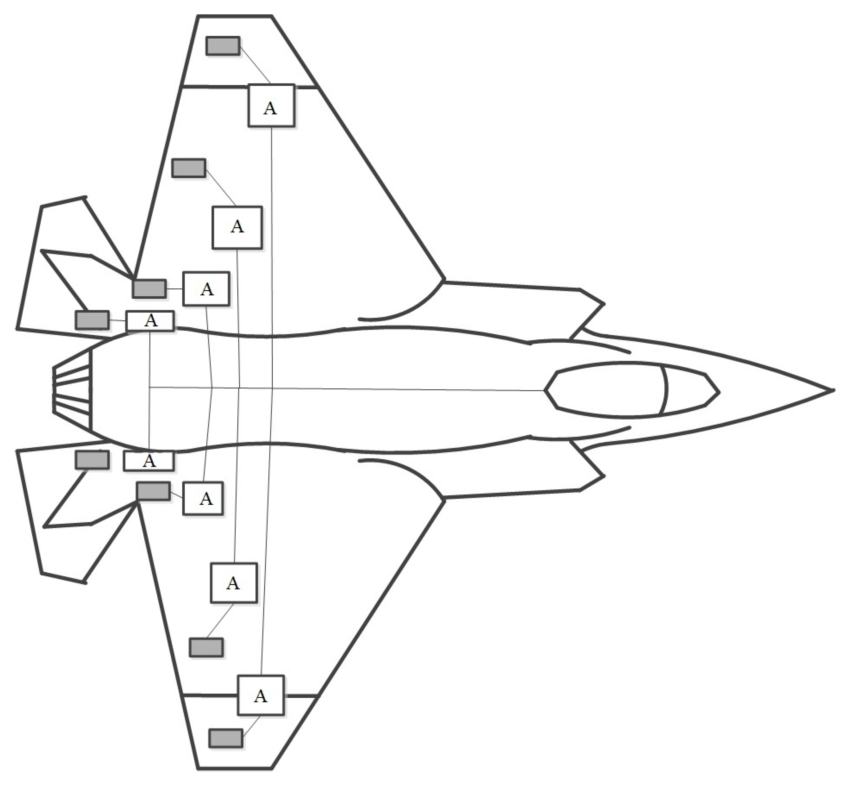
Figure 22 shows the distribution of rudders control units on the aircraft body.
ACPN functionally connects the aggregates to perform automatic control of flight stabilization processes. The spacing of the aggregates at a distance of several tens of meters makes it possible to synthesize control signals in the frequency range of 1 MHz. In this case, the wave properties of the connecting cables do not appear, and the design of the control system is simplified. Structural simplification of the control system makes it possible to increase its capabilities in the field of increasing reliability by connecting redundant communication channels.
4. Discussion
The article considers the theory of functional-logical processing of control signals by built-in analog computing devices.
The set goal of increasing the speed while reducing the mass-dimensional and energy indicators of a distributed control system is achieved by introducing an add-on in the form of analog calculators-agents into each aggregate. Agents, together with aggregates, form an analog cyber–physical network. With the help of the developed operations of continuum logic, the parametric, structural, and flow dynamics of the control system are significantly improved. At the same time, the computational process becomes an inseparable component of the physical processes occurring in the aggregates of the TS, since it is not associated with the transition to digital and software-algorithmic event processing.
The developed operations of continuum logic react to continuous changes in the processes in the TS, synthesizing commands for controlling the aggregates. Unlike the existing methods of continuum logic [29,30,31,32], in the proposed models, fuzzy calculations are replaced by deterministic ones. The negation operation is defined as in two-valued discrete logic, i.e., the logical laws of the excluded middle (tertium non datur) are fulfilled. Logic operations become an integral part of the continuum synthesis of control signals for aggregates. This allows:
- simultaneously process the states of the technical system and synthesize control signals;
- speed up the response of the control system to changes in the object’s parameters;
- reduce the design complexity, and improve the energy performance of the control system.
The approach to computing management is developing in the direction of unifying the element base, expanding the logical and algorithmic capabilities of analog devices. The technical result is the expansion of functionality, the unification of the structure of analog processors, and the increase in the efficiency of control of analog devices by switching from hybrid systems to ACPN.
Direct conversions of analog signals, parallel computing, and elimination of high-frequency digital processing make it possible to reduce the energy costs of ACPN by two orders of magnitude compared to digital distributed systems.
One of the promising areas of application for embedded ACPN is the analog processing of radio signals. With restrictions on weight and size characteristics and energy indicators, problems arise with the technical capabilities of digital systems. A report at the Systems of Signals Generating and Processing in the Field of on Board Communications Conference [33] presented a new approach to radio signal processing using an analog neurofilter. The task separation of signal from noise is solved using trainable analog neuron-like devices.
The advantages of the proposed approaches in technical systems of great complexity are demonstrated by the use of ACPNs for monitoring and diagnosing radio engineering complexes [34]. With a high intensity of transmission of the flow of information messages over communication lines, an overload of digital channels occurs. The transition to analog methods for processing control and diagnostic information and the integration of analog processors into control and diagnostic systems can significantly increase the depth and completeness of parameter control and increase the reliability of radio engineering complexes. By reducing the requirements for the frequency characteristics of communication channels in analog systems, it is possible to increase the intensity of polling sensors and the efficiency of monitoring components that are separated over long distances.
The use of hardware methods for synthesizing control functions and complex situational analysis of the states of the control object significantly speeds up the response of analog processors to ongoing events. In combination with low power consumption and weight and size characteristics, ACPNs are a promising basis for a control system for small robots and unmanned aerial vehicles.
The presented models of functional–logical signal processing in heterarchical chains of physical processors and parallel computing are an excellent solution for analog neural networks.
5. Conclusions
The performed studies allow us to draw theoretical and practical conclusions:
- (1)
- The possibilities of applying the theory of analog systems continuous logical analysis for obtaining deterministic solutions have been expanded. The developed models replace the fuzzy calculations used in continuum logic with logical operations of dividing decision-making areas into sub-areas, the boundaries of which are uniquely determined by the relationships between the instantaneous values of the parameters of the control object. The unambiguity of the decisions made increases the accuracy and reliability of the results of the situational analysis of the states of the vehicle in comparison with existing methods of continuous logic.
- (2)
- The presented generalized models of the logical analysis of the states of the TS allow systematizing the development of embedded analog devices for the distributed control of technical and technological objects that do not require: analog-to-digital conversions of sensor signals, programmable control devices and matching of embedded digital processors. The obtained hardware solutions are aimed at integrating computing processes into aggregates in order to create an ACPN, in which the synthesis of control signals of the TS takes place at low energy costs and the design complexity of the equipment.
- (3)
- The developed methods for the logical analysis of the states of the TS and the synthesis of control signals are implemented in analog devices based on continuum processors, which allow real-time (at a frequency of up to several tens of megahertz) of the operating modes of aggregates. Built-in CPs turn the TS into a distributed computing structure, in which analog computing is integrated with physical processes, leading to an increase in performance with a decrease in energy parameters due to the transition from sequential high-frequency digital calculations to continuous synthesis analog.
The declared properties of ACPNs open up prospects for their application in control systems for distributed TS, in artificial neural networks, micro-electromechanical, and microelectronic systems.
6. Patents
Patent for the invention of the Russian Federation No. 2739723 IPC G06G 7/00 (January 2006), G06F 7/00 Continuum Processor., Patent Library of the Russian Federation, 28 December 2020.
Funding
This research received no external funding.
Data Availability Statement
Data available in a publicly accessible repository.
Conflicts of Interest
The author declares no conflict of interest.
References
- Tortora, G.J.; Derrickson, B.H. Principles of Anatomy and Physiology; John Wiley & Sons: Hoboken, NJ, USA, 2018; 1248p. [Google Scholar]
- Helbling, E.F.; Fuller, S.B.; Wood, R.J. Altitude Estimation and Control of an Insect-Scale Robot with an Onboard Proximity Sensor. Robot. Res. 2018, 1, 57–69. [Google Scholar]
- Tanenbaum, A.S.; van Steen, M. Distributed Systems: Principles and Paradigms; Pearson Prentice Hall: Hoboken, NJ, USA, 2007; 686p. [Google Scholar]
- Sangiovanni-Vincentelli, A.L. Quo Vadis, SLD? Reasoning about the Trends and Challenges of System Level Design. Proc. IEEE 2007, 95, 467–506. [Google Scholar] [CrossRef]
- Goebel, R.; Sanfelice, R.G.; Teel, A.R. Hybrid Dynamical Systems. Modeling, Stability, and Robustness; Princeton University Press: Princeton, NJ, USA; Oxford, UK, 2012; 212p. [Google Scholar]
- Lee, E.A. Cyber-Physical Systems—Are Computing Foundations Adequate? Position Paper for NSF Workshop on Cyber-Physical Systems: Research Motivation, Techniques and Roadmap; Department of EECS, UC Berkeley: Austin, TX, USA, 2006; 9p. [Google Scholar]
- Henzinger, T.A. The theory of hybrid automata. In Verification of Digital and Hybrid Systems; NATO ASI Series; Springer: Berlin/Heidelberg, Germany; Electronics Research Laboratory College of Engineering University of California: Berkeley, CA, USA, 1996; Volume 170, pp. 265–292. [Google Scholar] [CrossRef]
- Broy, M. Functional specification of time-sensitive communicating systems. ACM Trans. Softw. Eng. Methodol. 1993, 2, 325–367. [Google Scholar] [CrossRef]
- Caferra, R. Logic for Computer Science and Artificial Intelligence; John Wiley & Sons: Hoboken, NJ, USA, 2013; 523p. [Google Scholar]
- Ball, S.R. Analog Interfacing to Embedded Microprocessor Systems; Real World Design, Newnes; Elsevier: Amsterdam, The Netherlands, 2004; 322p. [Google Scholar]
- Omar, Y. Ismael Analysis, Design, and Implementation of an Omnidirectional Mobile Robot Platform. Am. Sci. Res. J. Eng. Technol. Sci. 2016, 22, 195–209. [Google Scholar]
- Ashok, B.; Denis, A.S.; Kumar, C. Ramesh A review on control system architecture of a SI engine management system. Annu. Rev. Control 2016, 41, 94–118. [Google Scholar] [CrossRef]
- Baek, S.S.; Bermudez, F.G.; Fearing, R. Flight control for target seeking by 13 gram ornithopter. In Proceedings of the 2011 IEEE/RSJ International Conference on Intelligent Robots and Systems, San Francisco, CA, USA, 25–30 September 2011. 16p. [Google Scholar]
- Vijay, K.; Nathan, M. Opportunities and challenges with autonomous micro aerial vehicles. Int. J. Robot. Res. 2012, 31, 1279–1291. [Google Scholar]
- Sapaty, S.P. Military Robotics: Latest Trends and Spatial Grasp Solutions. Int. J. Adv. Res. Artif. Intell. 2015, 4, 9–18. [Google Scholar]
- Duhamel, P.-E.J.; Perez-Arancibia, N.O.; Barrows, G.L.; Wood, R.J. Biologically inspired optical-flow sensing for altitude control of flapping-wing microrobots. IEEE/ASME Trans. Mechatron. 2013, 18, 556–568. [Google Scholar] [CrossRef]
- De Wagter, C.; Tijmons, S.; Remes, B.D.; de Croon, G. Autonomous flight of a 20-gram flapping wing mav with a 4-gram onboard stereo vision system. In Proceedings of the 2014 IEEE International Conference on Robotics and Automation (ICRA), Hong Kong, China, 31 May–7 June 2014; pp. 4982–4987. [Google Scholar]
- Helbling, E.F.; Fuller, S.B.; Wood, R.J. Pitch and yaw control of a robotic insect using an onboard magnetometer. In Proceedings of the 2014 IEEE International Conference on Robotics and Automation (ICRA), Hong Kong, China, 31 May–7 June 2014; IEEE: Piscataway, NJ, USA, 2014; pp. 5516–5522. [Google Scholar]
- Harel, D.; Pnueli, A. On the development of reactive systems. In Logic and Models of Concurrent Systems; NATO Advanced Study Institute on Logic and Models for Verification and Specification of Concurrent Systems; Springer: Berlin/Heidelberg, Germany, 1985; pp. 477–498. [Google Scholar]
- Escoffier, C.; Finnigan, K. Reactive Systems in Java: Resilient, Event-Driven Architecture with Quarkus; O’Reilly Media: Sebastopol, CA, USA, 2022; 250p. [Google Scholar]
- Lee, B. Specification and Design of Reactive Systems; Memorandum No. UCB/ERL MOO/29; University of California: Berkeley, CA, USA, 2000; 126p. [Google Scholar]
- DeBole, M.V.; Taba, B.; Amir, A.; Akopyan, F.; Andreopoulo, A.; Risk, W.P.; Kusnitz, J.; Otero, C.O.; Nayak, T.K.; Appuswamy, R.; et al. TrueNorth: Accelerating From Zero to 64 Million Neurons in 10 Years. Computer 2019, 52, 20–29. [Google Scholar] [CrossRef]
- Davies, M.; Srinivasa, N.; Lin, T.-H.; Chinya, G.; Cao, Y.; Choday, S.H.; Dimou, G.; Joshi, P.; Imam, N.; Jain, S.; et al. Loihi: A Neuromorphic Manycore Processor with On-Chip Learning. IEEE Micro 2018, 38, 82–99. [Google Scholar] [CrossRef]
- Billaudelle, S.; Cramer, B.; Petrovici, M.A.; Schreiber, K.; Kappel, D.; Schemmel, J.; Meier, K. Structural plasticity on an accelerated analog neuromorphic hardware system. Neural Netw. 2021, 133, 11–20. [Google Scholar] [CrossRef] [PubMed]
- Vigoda, B. Analog Logic: Continuous-Time Analog Circuits for Statistical Signal Processing. Ph.D. Thesis, Massachusetts Institute of Technology, Cambridge, CA, USA, 2003; 209p. Available online: https://cba.mit.edu/docs/theses/03.07.vigoda.pdf (accessed on 23 June 2023).
- Chen, K.; Leu, J.; Gershenfeld, N. Analog Logic Automata. In Proceedings of the 2008 IEEE Biomedical Circuits and Systems Conference, Baltimore, MD, USA, 20–22 November 2008; pp. 189–192. [Google Scholar]
- Gershenfeld, N. Programming Bits and Atoms. In Proceedings of the 2013 IEEE 34th Real-Time Systems Symposium, Vancouver, BC, Canada, 3–6 December 2013; p. xiv. [Google Scholar]
- Gandharv, K. World’s First AI Analog Chip; Endless Origins: Delhi, India, 2021; Available online: https://analyticsindiamag.com/worlds-first-ai-analog-chip/ (accessed on 23 June 2023).
- Timothy, M. Continuous logic and embeddings of Lebesgue spaces. Arch. Math. Log. 2021, 60, 13. Available online: https://www.researchgate.net/publication/341687035_Continuous_logic_and_embeddings_of_Lebesgue_spaces#fullTextFileContent/ (accessed on 23 June 2023).
- Hanson, J. Continuous Logic for Discontinuous Logicians. 28 May 2023, p. 25. Available online: https://james-hanson.github.io/publications/ConLogDisLog.pdf (accessed on 23 June 2023).
- Li, X. The Classical Logic and the Continuous Logic. In Proceedings of the Future Technologies Conference (FTC), Vancouver, BC, Canada, 20–21 October 2022; Volume 1. Available online: https://www.researchgate.net/publication/364508302_The_Classical_Logic_and_the_Continuous_Logic (accessed on 23 June 2023).
- Li, X. The Continuous Logic; Department of Mathematics and Computer Science Alabama State University: Montgomery, AL, USA, 2015; p. 8. [Google Scholar] [CrossRef]
- Dembitsky, N.L.; Polyakov, S.V.; Timoshenko, A.V. Recognition of Analog Signals of a Given Shape Using Continuous Processors. In Proceedings of the 2020 Systems of Signals Generating and Processing in the Field of on Board Communications, Moscow, Russia, 19–20 March 2020; IEEE: Piscataway, NJ, USA; pp. 1–5. [Google Scholar]
- Dembitsky, N.L. Analog Self-Learning Automata of Radio Engineering Devices Based on Cyber-Physical Networks. In Proceedings of the 2022 Systems of Signals Generating and Processing in the Field of on Board Communications, Moscow, Russia, 15–17 March 2022; pp. 1–5. [Google Scholar]
Figure 1.
Diagram of the phase space of the technical system.
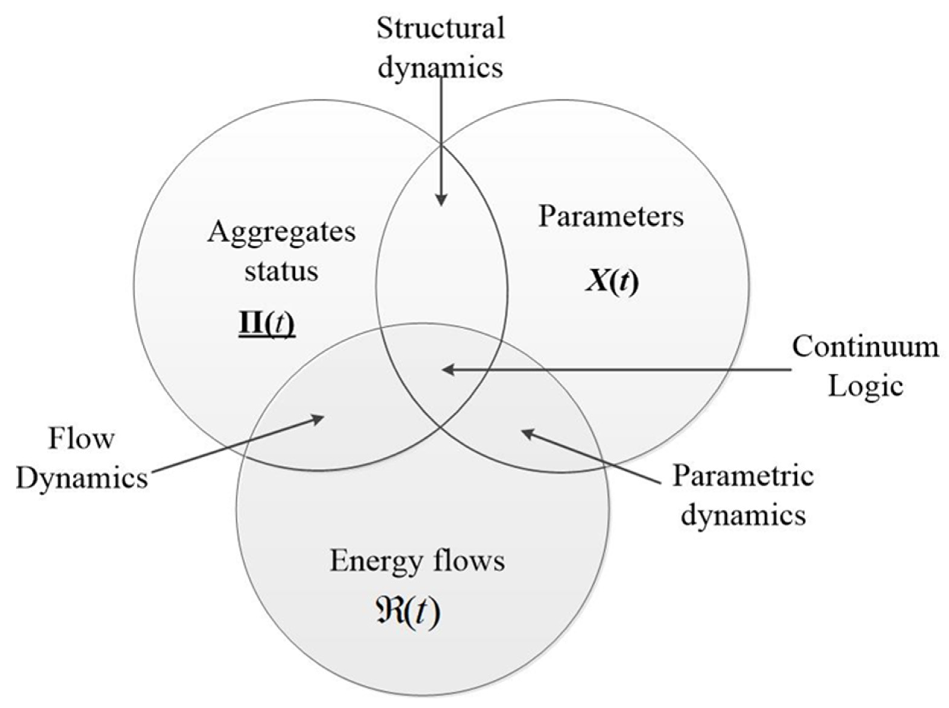
Figure 2.
The physical processor of the cyber–physical network. CPi—continuum processor.

Figure 3.
The heterarchical structure cyber–physical networks.
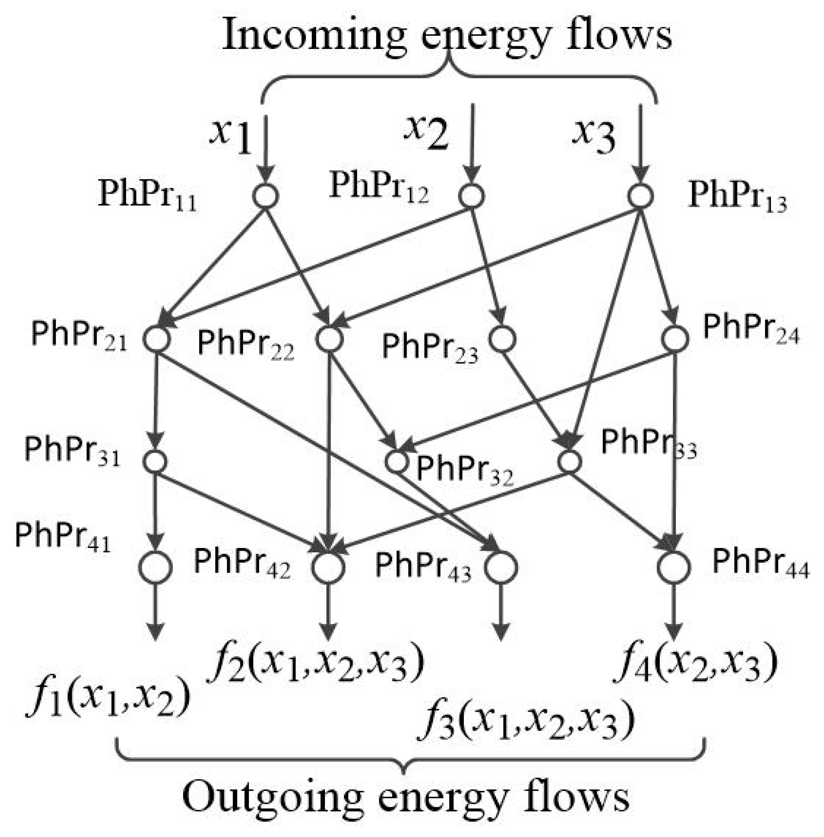
Figure 4.
Heterarchical structure of the cyber–physical network after blocking the aggregate in PhPr22.
Figure 4.
Heterarchical structure of the cyber–physical network after blocking the aggregate in PhPr22.

Figure 5.
Combining physical processors with incompatible outgoing EF.
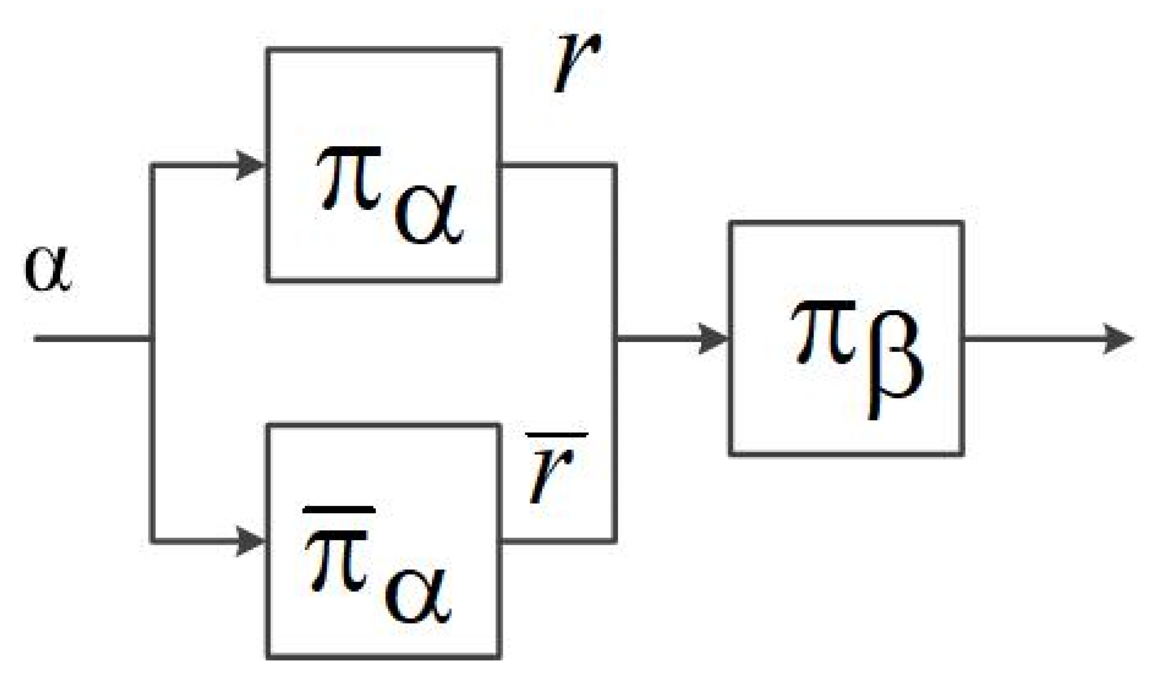
Figure 6.
Binary division of nodes in the ACPN.
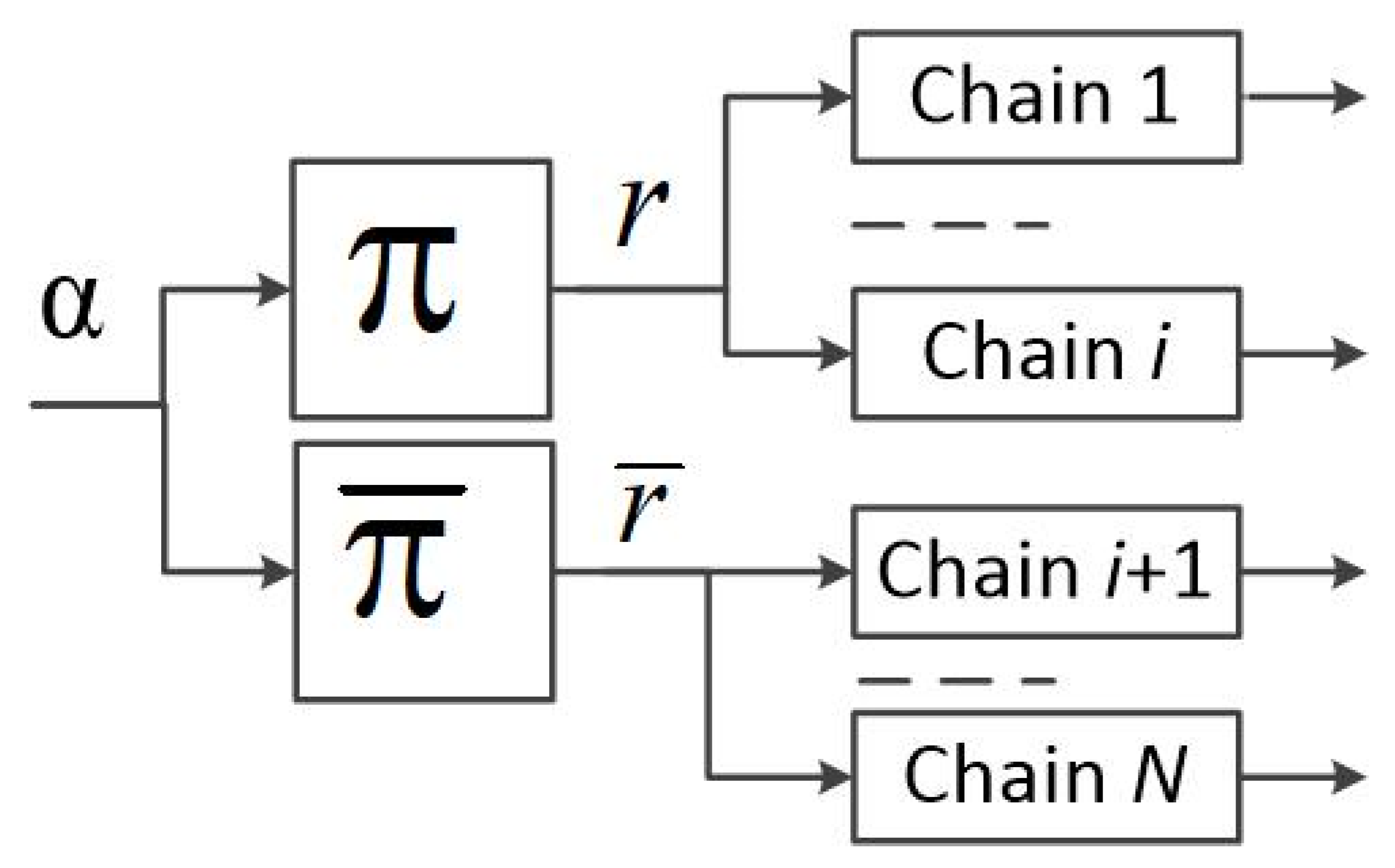
Figure 7.
Control of the operating modes of the aggregate in the PhPr: (a) domain of definition ; (b) domain of definition .
Figure 7.
Control of the operating modes of the aggregate in the PhPr: (a) domain of definition ; (b) domain of definition .

Figure 8.
Inversion of the parameters and of the boundaries of the regions.

Figure 9.
Element NOT in the analog network.

Figure 10.
Conjunctive operation for EF α and β: (a) domain of definition of conjunctive operation; (b) ACPN of conjunctive operation of EF α and β.
Figure 10.
Conjunctive operation for EF α and β: (a) domain of definition of conjunctive operation; (b) ACPN of conjunctive operation of EF α and β.

Figure 11.
Domain of definition of the disjunctive operation.
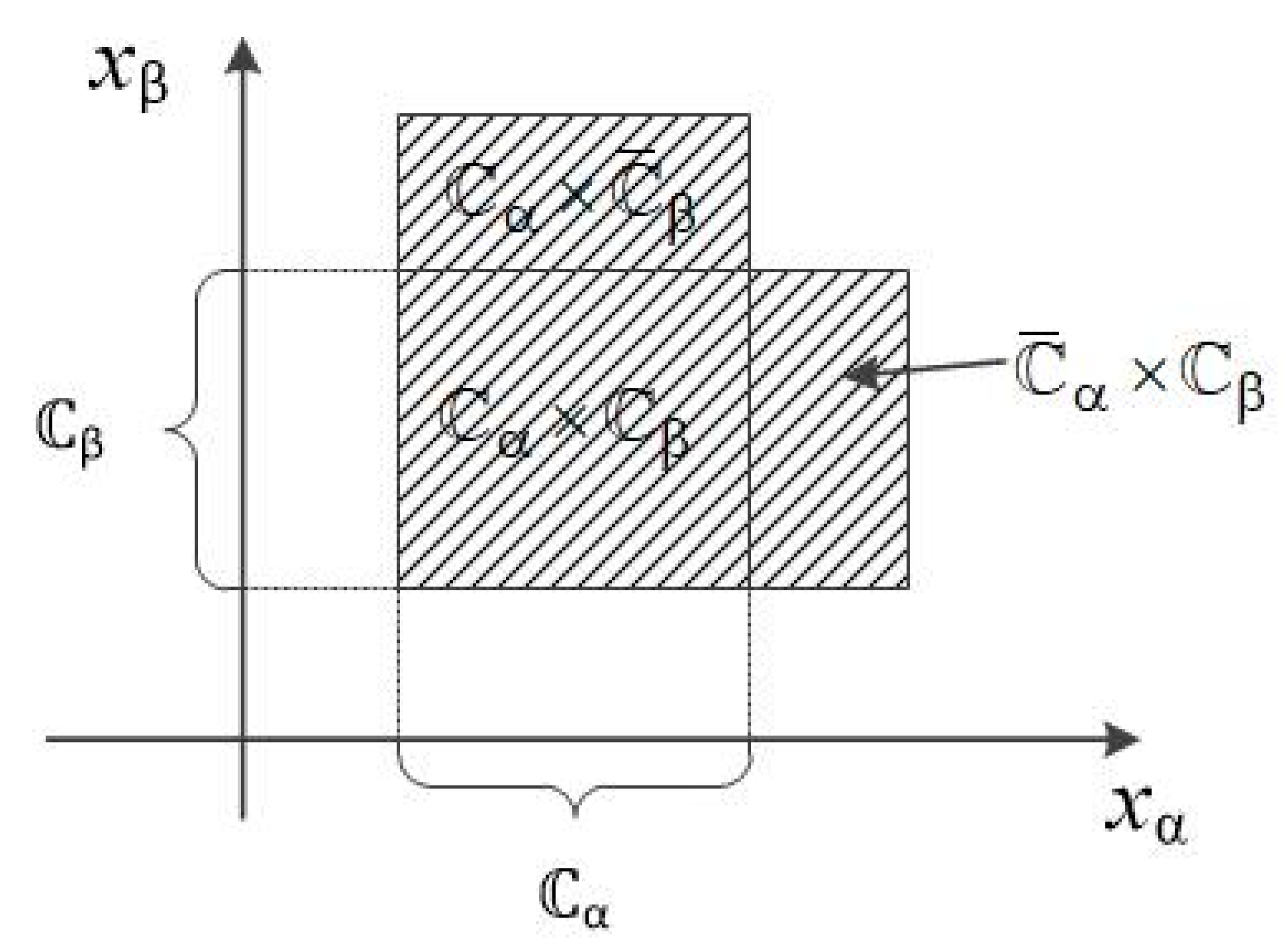
Figure 12.
ACPN of the disjunctive operation of EF α and β.
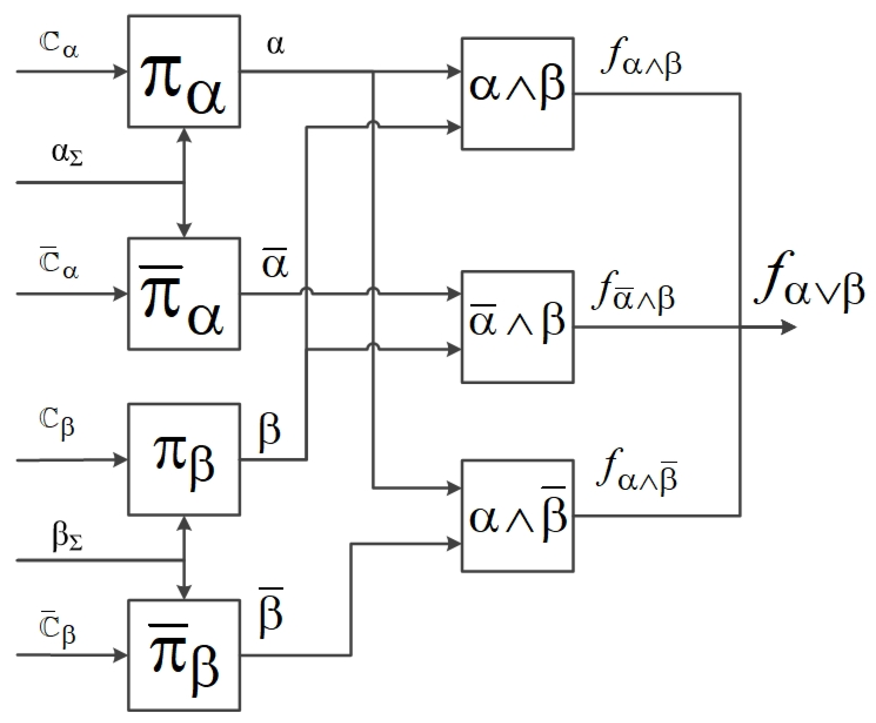
Figure 13.
ACPN of negation of the conjunctive operation of EF α and β.

Figure 14.
The domain of definition of EF α and β in the negation of conjunction operation.

Figure 15.
The domain of definition of EF α and β in the negation of disjunctive operation.

Figure 16.
The domain of definition of XOR operation.
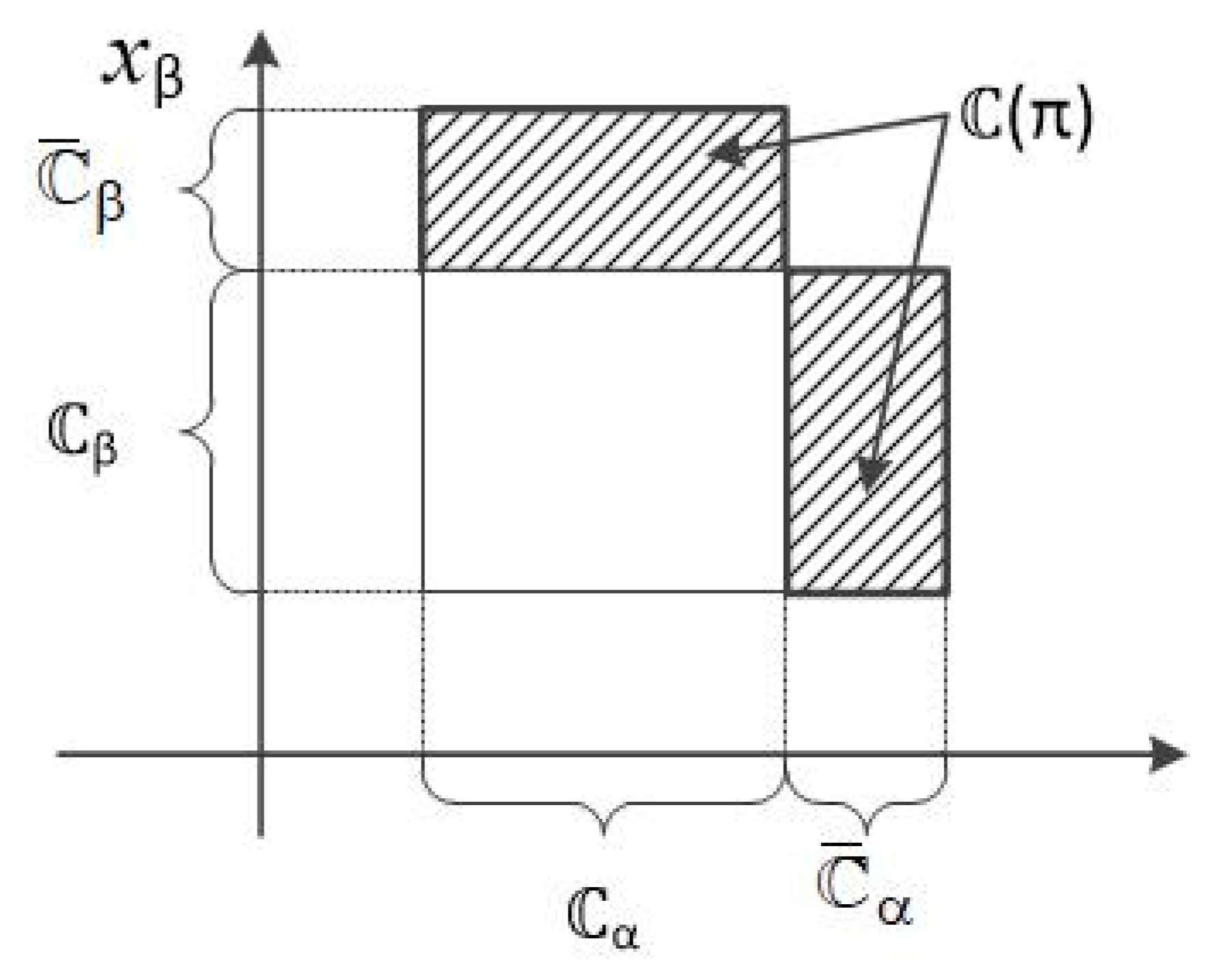
Figure 17.
ACPN of XOR operation of EF α and β.

Figure 18.
Image of a continuum processor on a circuit diagram.
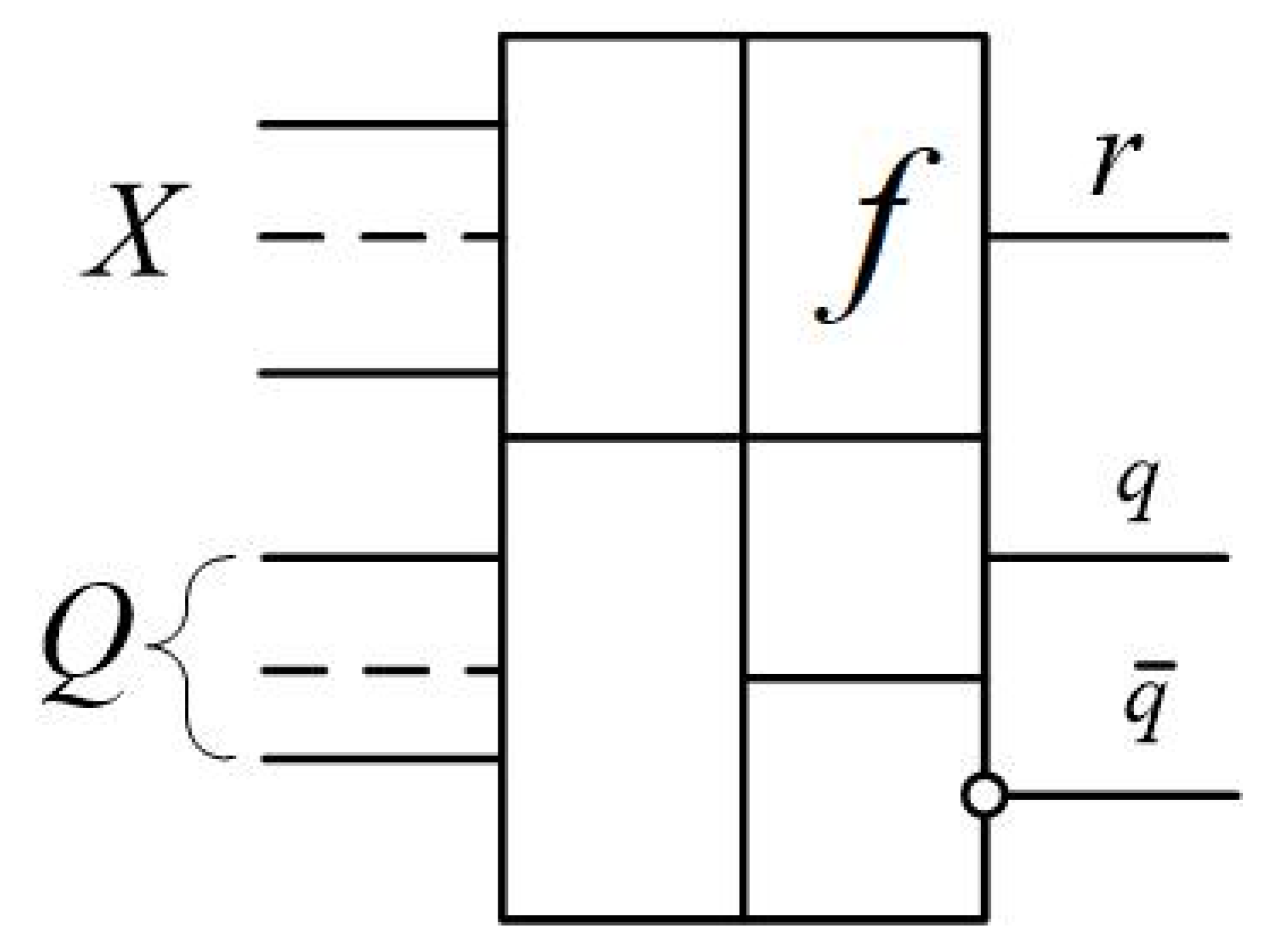
Figure 19.
CP connection in NOT operation.

Figure 20.
Connection CP in XOR operation of two analog signals.

Figure 21.
Agent–function selector on the continuum processors.
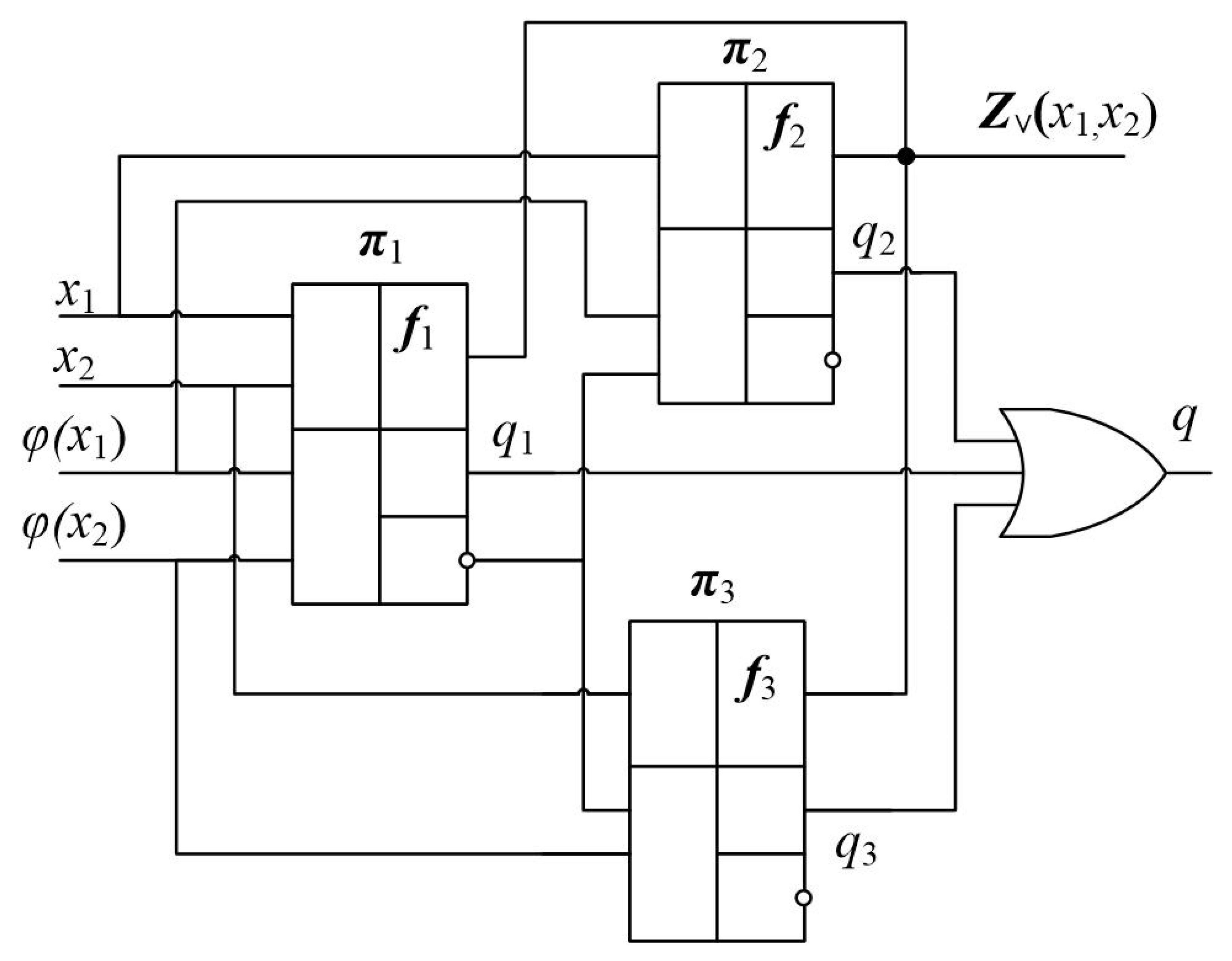
Figure 22.
Distribution of the rudders control aggregates and agents on the aircraft body. A—agents. Aggregates are shaded grey.
Figure 22.
Distribution of the rudders control aggregates and agents on the aircraft body. A—agents. Aggregates are shaded grey.
Disclaimer/Publisher’s Note: The statements, opinions and data contained in all publications are solely those of the individual author(s) and contributor(s) and not of MDPI and/or the editor(s). MDPI and/or the editor(s) disclaim responsibility for any injury to people or property resulting from any ideas, methods, instructions or products referred to in the content. |
© 2023 by the author. Licensee MDPI, Basel, Switzerland. This article is an open access article distributed under the terms and conditions of the Creative Commons Attribution (CC BY) license (https://creativecommons.org/licenses/by/4.0/).
Share and Cite
MDPI and ACS Style
Dembitsky, N. Continuum Logic of Control Signals in Analog Cyber–Physical Nets. Inventions 2023, 8, 101. https://doi.org/10.3390/inventions8040101
AMA Style
Dembitsky N. Continuum Logic of Control Signals in Analog Cyber–Physical Nets. Inventions. 2023; 8(4):101. https://doi.org/10.3390/inventions8040101
Chicago/Turabian StyleDembitsky, Nikolay. 2023. "Continuum Logic of Control Signals in Analog Cyber–Physical Nets" Inventions 8, no. 4: 101. https://doi.org/10.3390/inventions8040101