Article

Influence of Density Ratios on Richtmyer–Meshkov Instability with Non-Equilibrium Effects in the Reshock Process

1
School of Mathematics and Statistics & Key Laboratory of Analytical Mathematics and Applications (Ministry of Education) & Fujian Key Laboratory of Analytical Mathematics and Applications (FJKLAMA) & Center for Applied Mathematics of Fujian Province (FJNU), Fujian Normal University, Fuzhou 350117, China
2
Sino-French Institute of Nuclear Engineering and Technology, Sun Yat-sen University, Zhuhai 519082, China
*
Authors to whom correspondence should be addressed.
Inventions 2023, 8(6), 157; https://doi.org/10.3390/inventions8060157
Submission received: 30 October 2023 / Revised: 7 December 2023 / Accepted: 12 December 2023 / Published: 13 December 2023
(This article belongs to the Special Issue New Sights in Fluid Mechanics and Transport Phenomena)

Abstract

:
The Richtmyer–Meshkov instability in a two-component system during the reshock process for various density ratios is studied through the discrete Boltzmann method. Detailed investigations are conducted on both hydrodynamic and thermodynamic non-equilibrium behaviors. Specifically, the analysis focuses on the density gradient, viscous stress tensor, heat flux strength, thermodynamic non-equilibrium intensity, and thermodynamic non-equilibrium area. It is interesting to observe the complex variations to non-equilibrium quantities with the changing shock front, rarefaction wave, transverse wave, and material interface. Physically, the non-equilibrium area is extended as the perturbed material interface grows after the passing of the shock wave or secondary impact. Moreover, the global non-equilibrium manifestation decreases when the transmitted shock front and transverse waves leave or when the reflected rarefaction wave weakens. Additionally, the global thermodynamic non-equilibrium effect is enhanced as the physical gradients or non-equilibrium area increase. Finally, the local non-equilibrium effect decreases when the fluid structure gradually disappears under the action of dissipation/diffusion.

1. Introduction

The Richtmyer–Meshkov (RM) [1,2] instability is induced by a shock wave impacting a wrinkled material interface between two fluids. It is mainly due to the baroclinic effect caused by the non-coincidence of the density gradient and pressure gradient across the material interface [3]. The RM instability occurs frequently in nature and engineering applications, including supernova explosion [4], weapon implosion [5], aerospace [6], and inertial confinement fusion (ICF) [7,8]. Particularly, in the ICF process, the development of the RM instability is enhanced by multiple interactions between the incident shock wave and the material interface, which thereby limit the energy output [9]. In supersonic combustion engines, the RM instability accelerates contact between the fuel and oxidizer, thus enhancing the combustion rate [10]. Indeed, understanding the physical phenomenon of the RM instability is of great significance in the engineering field.
Recently, the RM instability induced by the secondary impact has become an active research topic and has produced fruitful results in theoretical [11,12,13] and experimental [14,15,16,17] studies. In particular, numerical simulation has promoted relative research due to its convenience and efficiency, and it can enrich our understanding of the RM instability from multiple perspectives. These perspectives are mainly attributed to the following three levels: macroscopic [18,19,20,21,22,23,24], microscopic [25,26], and mesoscopic aspects [27,28,29]. In the macroscopic view, various codes based on hydrodynamic governing equations, such as Euler or Navier–Stokes equations, have been widely used to simulate fluid instability. For example, in 2011, Ukai et al. [18] employed the compressible Navier–Stokes equations to study the growth of the RM instability during the reshock process for various interface shapes. In 2014, Tritschler et al. [19] explored the RM instability at the deterministic multimode interface and found that the vorticity deposition produced by the secondary impact material interface is greater than that of the primary impact. In 2019, Li et al. [21] studied the RM instability with reshock in the interaction between the mixing zone and multiple waves by using a direct numerical simulation and found that the mixing zone is accelerated by rarefaction and compression waves alternatively with decaying strength after reshock. In 2021, Bin et al. [23] successfully captured the growth of the RM instability mixed width under reshock and spatial structure in three dimensions by constrained large-eddy simulations. In 2022, Mohaghar et al. [24] performed three-dimensional simulation of the reshocked inclined RM instability turbulent mixing layer under single-mode and multimode configurations through Flash code and discovered that the growth of the mixing layer depends on the initial perturbation. Moreover, in the microscopic view, Wu et al. [25] utilized classical molecular dynamics to investigate the microscopic-scale RM instability of a single-mode Cu–He interface subjected to a cylindrically converging shock in 2018. Later, in 2020, Liu et al. [26] investigated the circulation deposition processes under different initial conditions by a direct simulation Monte Carlo method; they found the viscosity gradient in the region of interaction increases with an increase in the shock strength, and the incident shock Mach number determines the relative contribution of the viscous source. Although these microscopic approaches can provide insight into the RM instability, they are limited to small-scale problems due to the high cost of computational resources.
Fortunately, the mesoscopic method can provide a bridge between the macroscopic and microscopic approaches and can resolve the contradiction between physical accuracy and calculation speed. Recently, the discrete Boltzmann method (DBM) has become an important tool for studying complex fluid systems at the mesoscopic level. Based upon non-equilibrium statistical physics, the DBM not only recovers fluid equations at the hydrodynamic limit, it also provides thermodynamic non-equilibrium (TNE) information beyond that of traditional macroscopic models [30,31]. In fact, the DBM is a variant version of the lattice Boltzmann method, which has been widely used as a solver of the Navier–Stokes equations and other partial differential equations [32,33,34,35,36,37,38]. As a coarse-grained physical method, the DBM can capture abundant hydrodynamic and TNE behaviors and describe the evolution of sharp interfaces, small-scale structures, and rapidly changing modes in fluid systems. For instance, in 2014, Lin et al. [27] presented a polar-coordinate DBM for compressible flows, simulated the RM instability induced by a shock wave traveling outwards through a heavier (lighter) medium to a lighter (heavier) medium, and analyzed the non-equilibrium manifestations around the material and mechanical interfaces. In 2018, Chen et al. [28] used the multiple-relaxation-time DBM to investigate the non-equilibrium characteristics of a coexistence system involving both RM and Rayleigh–Taylor instability and found that the non-equilibrium effect of the system increases as the Mach number increases, while the effect of gravity acceleration on the non-equilibrium characteristics is different at various phases. In 2023, Shan et al. [29] employed the two-fluid DBM to investigate the non-equilibrium kinetic effects on the RM instability and reshock process and found that lighter fluid has a higher entropy production rate than heavier fluid. Moreover, the DBM also provides new insights for complex fluid systems, such as hydrodynamic instability [39,40,41,42,43], multiphase flow [44,45], reactive flow [46], etc.
It is noteworthy that the Atwood number has attracted great attention because it plays a crucial role in the RM instability. Early in 1960, under the assumptions of a small disturbance and incompressible fluid, Richtmyer proposed a linear growth model that revealed a positive correlation between the growth rate of a perturbation and the Atwood number [1]. In 2011, Lombardini et al. [47] found that the evolution of mixed regions showed irregularities with an increasing Atwood number in the process of the RM instability. In 2016, Zhou et al. [48] investigated the RM instability under single and secondary shocks for various Atwood numbers and found that for the secondary shock, the larger the Atwood number, the smaller the normalized mixed mass. In 2019, Chen et al. [49] systematically analyzed the influence of the Atwood number on the RM instability for slightly perturbed interfaces in elastic–plastic media. In the same year, Liao et al. [50] studied the RM instability driven by a perturbed shock wave and found that the amplitude of the material interface decreases with the increasing Atwood number. In 2021, Tang et al. [51] adopted the Euler equations to study the single-mode RM instability induced by the convergent shock wave and observed that the amplitude perturbation grows more rapidly and the nonlinearity becomes more pronounced as the Atwood number increases. In 2022, Ren et al. [52] used the hydrocode Pagosa to explore the multimode RM instability with a variety of initial conditions, including differing the number of modes, Atwood number, and perturbation type. Up to now, the study of the Atwood number or density ratio has mainly involved the macroscopic aspect. In fact, in the RM instability process, the interaction between the shock wave and material interface also results in abundant and pronounced TNE behavior. Unfortunately, these behaviors are inappropriately ignored due to the limitations of computational models.
To further study the hydrodynamic non-equilibrium and TNE effects of the RM instability in the reshock process for various density ratios, the two-component DBM [53] is employed in this work. The structure of this paper is as follows: In Section 2, the DBM is briefly introduced. In Section 3, we simulate the RM instability and discuss its evolution mechanism in detail. Finally, a conclusion is given in Section 4.

2. Two-Component Discrete Boltzmann Model

The discrete Boltzmann equation for a two-component fluid system takes the following form [53]:
f i σ t + v i · f i σ r = Ω i σ ,
where σ ( = A , B ) represents chemical species, i ( = 0 , 1 , , N ) is the index of discrete velocities, f i σ ( f i σ e q ) is the discrete (equilibrium) distribution function of each component, t is the time, v i is the discrete velocity, and r is the space coordinate. The collision term Ω i σ is calculated as
Ω i σ = 1 τ σ ( f i σ f i σ e q ) ,
where the relaxation time τ σ = ( n A / θ A + n B / θ B ) 1 , and θ A and θ B are the relaxation parameters. The number density n σ , mass density ρ σ , and flow velocity u σ of each component are expressed by
n σ = i f i σ ,
ρ σ = n σ m σ ,
u σ = 1 n σ i f i σ v i ,
where m σ represents the molecular mass of σ . The mixing number density n, mass density ρ , and flow velocity u are
n = σ n σ ,
ρ = σ ρ σ ,
u = 1 ρ σ ρ σ u σ .
The internal energy density of each component and the internal energy density of the system are
E σ = 1 2 m σ i f i σ [ | v i u | 2 + η i 2 ] ,
E = σ E σ ,
where the symbol η i is used to describe the internal energy density for extra degrees of freedom. Let us introduce D and I, which represent the spatial dimension and extra degrees of freedom, respectively, and choose D = 2 and I = 3 in this paper. Then the individual temperature T σ and mixing temperature T can be calculated as
T σ = 2 E σ n σ ( D + I ) ,
T = 2 E n ( D + I ) .
Via the Chapman–Enskog expansion, it is proved that the Navier–Stokes equations can be recovered from Equation (1) in the continuum limit: see details in Appendix A. To this end, f i σ e q should satisfy seven kinetic moments: see Appendix B. Those relationships can be written in the following matrix form:
C · f σ e q = f ^ σ e q ,
in terms of
f σ e q = [ f 1 σ e q , f 2 σ e q , , f N σ e q ] T ,
f ^ σ e q = [ f ^ 1 σ e q , f ^ 2 σ e q , , f ^ N σ e q ] T ,
with an N × N matrix C = [ C 1 , C 2 , , C N ] T that links moment space to velocity space, and the elements within C are determined by the discrete velocity model. From Equation (13), the discrete equilibrium distribution function of each component can be obtained
f σ e q = C 1 · f ^ σ e q ,
where C 1 is the inverse matrix of C .
It is noteworthy that the first three kinetic moments in Equations (A6)–(A8) are related to the conservation of mass, momentum, and energy, respectively. Consequently, f i σ e q can be replaced by f i σ in those three formulas. However, in Equations (A9)–(A12), if f i σ e q is replaced by f i σ , the values of the left and right sides may deviate. In fact, the deviation of the non-conservation moments of f i σ and f i σ e q can be used to measure the degree of departure from the equilibrium state of the system, which is the core and purpose of the DBM. To be specific, the symbols M m , n σ ( f i σ ) and M m , n σ ( f i σ e q ) are introduced to stand for the central kinetic moments of f i σ and f i σ e q , respectively. Here “ m , n ” denotes that the m-order tensor is contracted to the n-order tensor. Both M m , n σ ( f i σ ) and M m , n σ ( f i σ e q ) are functions of the peculiar velocity v i = v i u . Then, the non-equilibrium quantities are defined as
Δ m , n σ = M m , n σ ( f i σ ) M m , n σ ( f i σ e q ) .
To better describe the global TNE of the fluid system, several TNE quantities are defined below:
| Δ 2 σ | = | Δ 2 x x σ | 2 + | Δ 2 x y σ | 2 + | Δ 2 y y σ | 2 ,
| Δ 3 , 1 σ | = | Δ 3 , 1 x σ | 2 + | Δ 3 , 1 y σ | 2 ,
| Δ 3 σ | = | Δ 3 x x x σ | 2 + | Δ 3 x x y σ | 2 + | Δ 3 x y y σ | 2 + | Δ 3 y y y σ | 2 ,
| Δ 4 , 2 σ | = | Δ 4 , 2 x x σ | 2 + | Δ 4 , 2 x y σ | 2 + | Δ 4 , 2 y y σ | 2 ,
| Δ σ | = | Δ 2 σ | 2 + | Δ 3 , 1 σ | 2 + | Δ 3 σ | 2 + | Δ 4 , 2 σ | 2 ,
where Δ 2 σ denotes the non-organized momentum flux and is related to the viscosity, Δ 3 , 1 σ and Δ 3 σ represent the non-organized energy flux and are associated with the heat flux, and Δ 4 , 2 σ indicates the flux of the non-organized energy flux.
By integrating several TNE quantities and then calculating the average over the whole computational region L x × L y , where L x and L y indicate the length and width of the fluid system, the average TNE intensities can be obtained as below:
D ¯ 2 σ = 1 L x L y 0 L x 0 L y | Δ 2 σ | d x d y ,
D ¯ 3 , 1 σ = 1 L x L y 0 L x 0 L y | Δ 3 , 1 σ | d x d y ,
D ¯ 3 σ = 1 L x L y 0 L x 0 L y | Δ 3 σ | d x d y ,
D ¯ 4 , 2 σ = 1 L x L y 0 L x 0 L y | Δ 4 , 2 σ | d x d y ,
D ¯ σ = 1 L x L y 0 L x 0 L y | Δ σ | d x d y .
These average TNE intensities describe the overall non-equilibrium effects of the system from different perspectives.
In addition, for the discretization of the velocity space, we adopt the discrete velocity model D2V16 that takes the following form [46]:
v i = v a cos ( i 1 ) π 2 , sin ( i 1 ) π 2 , 1 i 4 , v b cos ( 2 i 1 ) π 4 , sin ( 2 i 1 ) π 4 , 5 i 8 , v c cos ( i 9 ) π 2 , sin ( i 9 ) π 2 , 9 i 12 , v d cos ( 2 i 9 ) π 4 , sin ( 2 i 9 ) π 4 , 13 i 16 ,
where v a , v b , v c , and v d are flexible parameters; η i = η a for 1 i 4 , η i = η b for 5 i 8 , η i = η c for 9 i 12 , η i = η d for 13 i 16 ; and η a , η b , η c , η d are tunable parameters. Furthermore, the first-order forward Euler scheme is adopted for the time derivative, and the second-order nonoscillatory and nonfree-parameter dissipation difference scheme is adopted for the space derivatives [54]. Additionally, all physical quantities are dimensionless in this paper [40]. In fact, dimensionless quantities can be converted from/to dimensional physical quantities, which is a technique that is widely used in both the discrete Boltzmann method [40,55] and the lattice Boltzmann method [56,57,58,59].

3. Results and Discussions

In this section, let us perform two-dimensional simulations of the RM instability in the reshock process within a region L x × L y = 0.5 × 0.1 . Figure 1 delineates the initial configuration of the RM instability as follows:
( ρ , u x , u y , p ) L = ( 1.3416 , 0.3615 , 0.0 , 1.5133 ) , ( ρ , u x , u y , p ) M = ( 1.0 , 0.0 , 0.0 , 1.0 ) , ( ρ , u x , u y , p ) R = ( ρ R , 0.0 , 0.0 , 1.0 ) ,
where the subscripts L and M represent the left and middle regions, respectively, which are filled with species A, and R stands for the right area, which is full of B. The shock wave is initially located at x = 0.025 between the left and middle regions, and it propagates rightwards with a Mach number Ma = 1.2 . (The current research is based on a relatively small Mach number, and other cases for larger Mach numbers may be considered in the future.) The physical quantities across the shock wave satisfy the Rankine–Hugoniot relations [60]. Further, a perturbation in the material interface at around x = 0.125 separates the M part from the R part. To stimulate the growth of the RM instability, a sinusoidal perturbation function is applied to the material interface, y = 0.125 + A 0 cos ( k y ) , in terms of the perturbation amplitude A 0 = 0.01 and the wave number k = 2 π / L y . Moreover, to ensure the fluid system is in mechanical and thermal equilibrium initially, the pressures and temperatures of components A and B are the same alongside the material interface, and the concentrations of the two species are chosen as n A = n B = 1 here. Consequently, the density ratio between them is
r = ρ R ρ M = ρ B ρ A = n B m B n A m A = m B m A .
In addition, the Atwood number is defined as
A t = ρ R ρ M ρ R + ρ M = r 1 r + 1 .
It can be found that there is a relationship between the density ratio and the Atwood number. In this paper, without loss of generality, we give a fixed m A = 1 and a tunable m B . Accordingly, the density ρ R in Equation (29) and the density ratio r in Equation (30) are flexible. In addition, we choose the relaxation parameters θ A = θ B = 2.0 × 10 5 , and other parameters ( v a , v b , v c , v d ) = ( 0.6 , 1.6 , 2.9 , 5.9 ) and ( η a , η b , η c , η d ) = ( 0.0 , 2.9 , 0.0 , 0.0 ) . The periodic boundary condition is used on the top and bottom, the inlet boundary condition is used on the left, and the symmetrical boundary condition is used on the right.

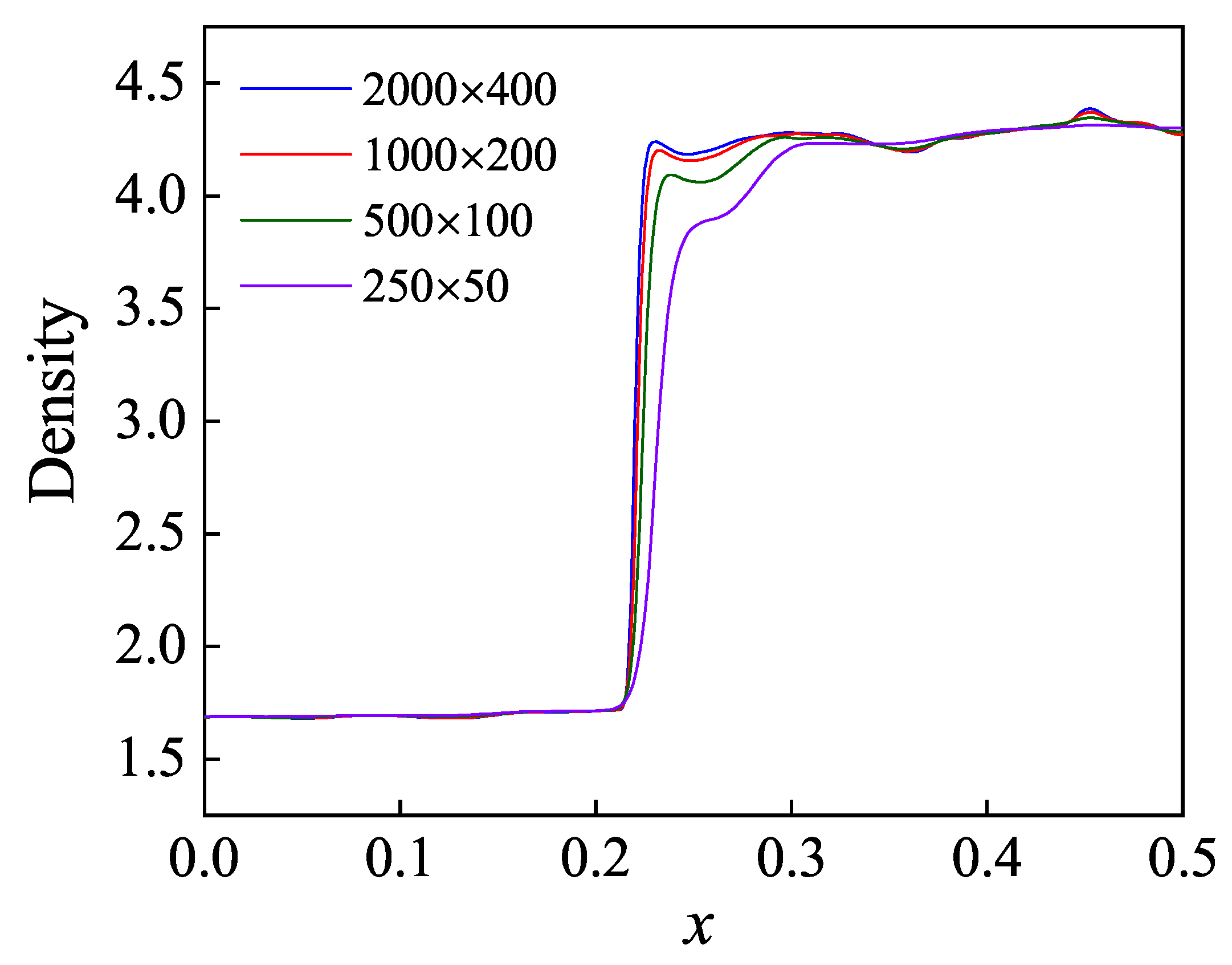
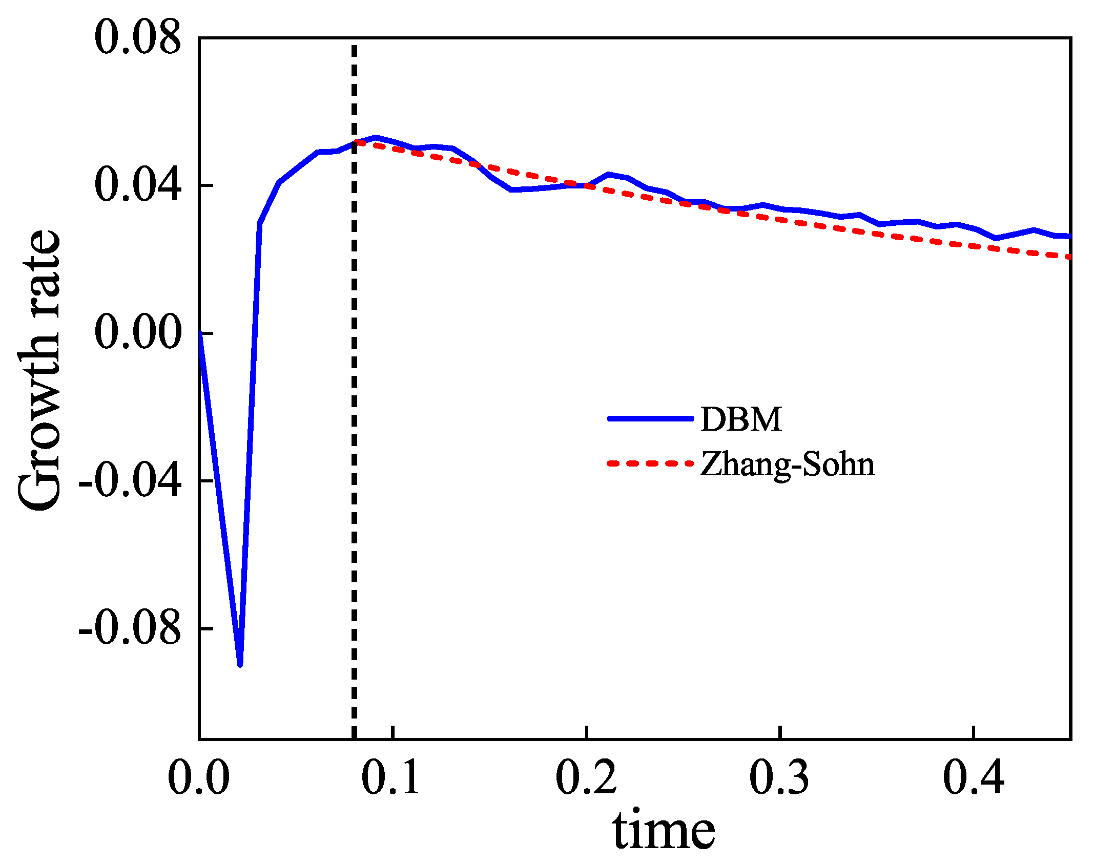
3.1. Verification and Validation

First of all, the grid-independent test is performed: see details in Appendix C. For the sake of effective and accurate simulation, we choose mesh grids of N x × N y = 2000 × 400 , a space step Δ x = Δ y = 2.5 × 10 4 , and a time step Δ t = 5.0 × 10 6 . Then, to further validate the DBM for the simulation of the RM instability, a comparison is made between the DBM and the Zhang–Sohn model [61]. Mathematically, the theoretical solution of the overall amplitude growth from the early to the late stage is predicted by the Zhang–Sohn model as follows [61]:
v = v 0 1 + v 0 a 1 k 2 t + max [ 0 , a 1 2 k 2 A 1 2 + 0.5 ] v 0 2 k 2 t 2 ,
where a 1 is the post-shock amplitude, A 1 is the post-shock Atwood number, and v 0 = k Δ u A 1 a 1 , with Δ u denoting the change in the interface velocity caused by the shock wave. Figure 2 delineates the perturbation growth rates under the condition of ρ R = 2.5 . The solid and dashed lines stand for the numerical and theoretical results, respectively. The shock front encounters the material interface at the time instant t = 0.0 and compresses it subsequently, so the simulated growth rate is less than zero in the early stage. After the time t = 0.08 , the shock wave departs from the material interface, the perturbed interface increases, and its growth rate is greater than zero. As time goes on, the growth rate decreases gradually. From Figure 2, it can be seen that the DBM results agree with the theoretical solutions of the Zhang–Sohn model [61] for the evolution of the RM instability, indicating the reliability of the present numerical method.
For an intuitive understanding of the evolution of the RM instability, Figure 3 illustrates the snapshots for the case r = 2.5 at different moments: the contours of the density, non-equilibrium strength, and vorticity are plotted in the three columns from left to right, respectively. Clearly, in the first column, the shock wave propagates from light to heavy fluids in the early state. At t = 0.1 , the shock wave first passes through the material interface, producing a leftward reflected shock wave and a rightward transmitted shock wave. The transmitted shock wave reaches the right boundary then is reflected and propagates leftwards from t = 0.3∼0.7. At about t = 0.7 , the secondary shock wave interacts with the material interface; then, the reflected rarefaction wave enters the heavier fluid and the transmitted shock wave enters the lighter fluid. Meanwhile, transverse waves are generated as a result of the impact of the shock wave on the wrinkled material interface and are continuously elongated, forming remarkable crisscrossing patterns. Afterward, the material interface starts to deform, and both the peak and valley shift into each other. This is also one of the classical phenomena of the RM instability. When t > 1.3 , the two components penetrate each other, creating “bubble” and “spike” structures, and the “spike” structure gradually evolves into the “mushroom” structure. Finally, as the fluid is fully mixed, the fine fluid structure slowly disappears. These phenomena are qualitatively consistent with previous experimental and numerical studies [14,22].
Further, it is apparent in the second column of Figure 3 that the fine fluid structures can be vividly depicted by the non-equilibrium contours. Here, the non-equilibrium strength is calculated by summing the TNE intensity of each component, i.e., | Δ | = | Δ A | + | Δ B | . At the initial moment, the system is in equilibrium with f i σ = f i σ e q ; hence, | Δ A | + | Δ B | = 0 . Afterwards, this TNE manifestation becomes larger than zero ( | Δ | > 0 ) because of the dissimilarity between f i σ and f i σ e q . When the (reflected transmitted) shock wave passes through the material interface, it leads to a sudden surge in the TNE strength. Subsequently, the RM instability continues to evolve, the material interface is elongated, and the non-equilibrium region increases. As the two components are fully mixed, the material interface is gradually blurred, and the fluid system tends to equilibrium eventually.
In addition, the last column in Figure 3 displays the vorticity in the evolution of the RM instability. Here, the vorticity is mathematically expressed by
ω = u y x u x y ,
and physically it is closely related to the flow-field structure and can reflect the deformation of the material interface. In the initial stage, symmetry and a small vortex structure begin to appear around the material interface due to the velocity difference between two sides of the material interface. With the evolution of the RM instability, the vortex structure develops, which further promotes the deformation and elongation of the material interface. These simulation results are qualitatively consistent with previous studies [22,62].
To gain insight into the evolution of the RM instability with different density ratios, we show the case of r = 5.0 in Figure 4. Similar to the process in Figure 3, the linear, non-linear, deformation, and mixing stages of the RM stability can also be observed in Figure 4. Different from the case in Figure 3, here, the transmitted shock wave travels slower in component B in the period of t = 0.1∼0.8. As shown in Figure 4, after t > 1.0 , the evolution speed of the material interface is accelerated significantly, leading to a more remarkable structural change and a more complex flow field. All the above numerical results agree with previous research [51,63].

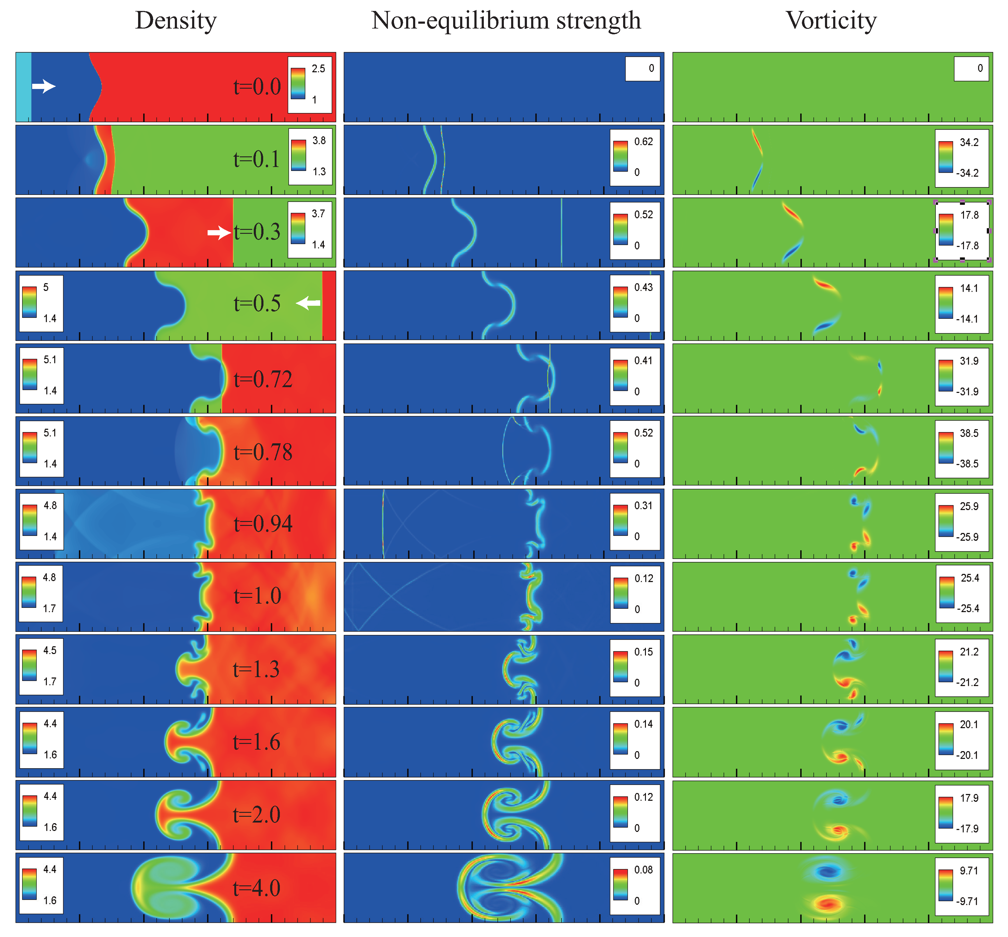
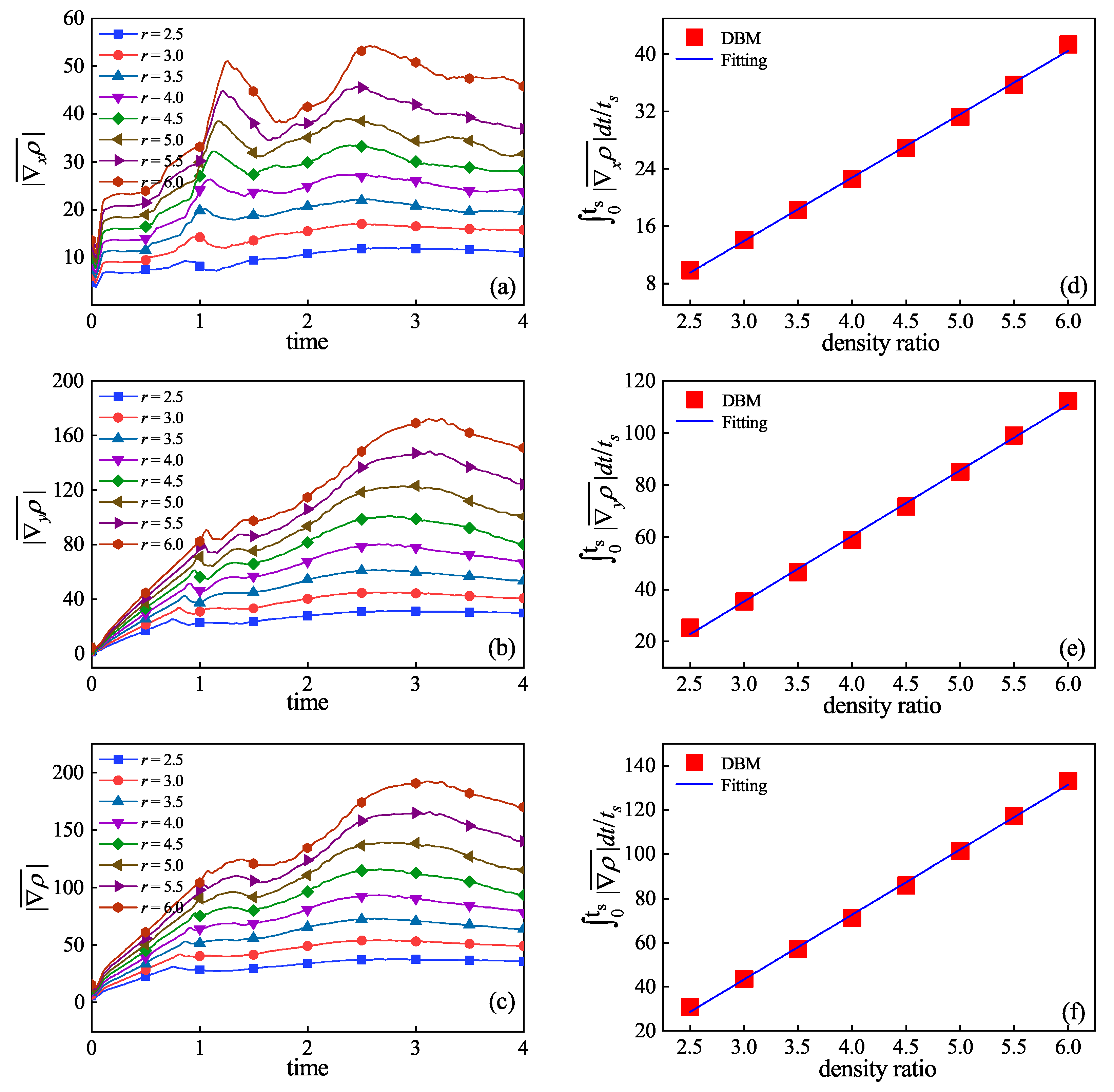
3.2. Hydrodynamic Non-Equilibrium Effects

Next, let us study the hydrodynamic non-equilibrium behavior in the evolution of the RM instability. For this purpose, we introduce the average density gradients as below:
| x ρ ¯ | = 1 L x L y 0 L x 0 L y | ρ x | d x d y ,
| y ρ ¯ | = 1 L x L y 0 L x 0 L y | ρ y | d x d y ,
| ρ ¯ | = 1 L x L y 0 L x 0 L y | ρ x | 2 + | ρ y | 2 d x d y ,
where the integral is over the whole computational region. Physically, | x ρ ¯ | and | y ρ ¯ | stand for the average density gradients in the x and y directions, respectively. The average density gradient | ρ ¯ | increases with increasing | x ρ ¯ | or | y ρ ¯ | .
Figure 5a–c show the evolution of the average density gradients | x ρ ¯ | , | y ρ ¯ | , and | ρ ¯ | , respectively. The lines with different symbols denote the results for various density ratios, i.e., r = 2.5 , 3.0 , ⋯, 6.0 , respectively. It can be found in Figure 5a that the tendency of | x ρ ¯ | is similar in each case. Take the case with r = 5.0 : the shock wave impacts the material interface from t = 0.04 to 0.1 , leading to a rapid upward trend of | x ρ ¯ | . Then, | x ρ ¯ | continues to rise and reaches the peak for the first time at t = 1.2 , when the density gradient across the material interface, shock wave, rarefaction wave, and transverse waves all together contribute to the maximum of | x ρ ¯ | . From t = 1.2 to 1.5 , | x ρ ¯ | shows a downward trend because the transmitted shock wave and transverse waves begin to leave the computational domain, although the material interface undergoes a reversal. Subsequently, from t = 1.5 to 2.4 , the RM instability continues to evolve, the material interface is elongated, the physical field becomes complex, and | x ρ ¯ | rises again. Finally ( t > 2.4 ), the material interface gradually becomes blurred due to the effects of dissipation/diffusion; the physical field becomes smoother, leading to a decrease in | x ρ ¯ | .
From Figure 5b, it can be observed that the evolution of the average density gradient in the y direction | y ρ ¯ | is different from that of | x ρ ¯ | . Before the time t = 1.0 , under the influence of the RM instability, the sum of the material surface and mechanical interface increases in the y direction; hence, the global density gradient in the y direction rises. Subsequently, | y ρ ¯ | decreases due to the interface reversal when the length of the contact interface decreases. During the stage of t = 1.1∼2.7, the length of the material interface increases because of the RM instability, so | y ρ ¯ | rises again. Finally ( t > 2.7 ), as the fluids are fully mixed, the fine structure gradually disappears, the system tends to reach equilibrium, and | y ρ ¯ | decreases.
Moreover, as shown in Figure 5c, it is easy to understand the tendency of | ρ ¯ | through analysis of the variation to | x ρ ¯ | and | y ρ ¯ | . Moreover, to have a deeper insight into the law of density gradients, the second column of Figure 5 shows the results of 0 t s | x ρ ¯ | d t / t s , 0 t s | y ρ ¯ | d t / t s , and 0 t s | ρ ¯ | d t / t s , where the integral is conducted over the period from t = 0 to t s , and the final instant is chosen at t s = 4 in this paper. Physically, the three quantities reflect the time-integration results of | x ρ ¯ | , | y ρ ¯ | , and | ρ ¯ | , respectively. The fitting functions are 0 t s | x ρ ¯ | d t / t s = 12.58 + 8.84 r , 0 t s | y ρ ¯ | d t / t s = 40.04 + 25.14 r , and 0 t s | ρ ¯ | d t / t s = 44.81 + 29.37 r , respectively. It is interesting to observe that each of the three quantities ( 0 t s | ρ ¯ | d t / t s , 0 t s | x ρ ¯ | d t / t s , and 0 t s | y ρ ¯ | d t / t s ) show a linear relationship with the density ratio. Physically, as the density ratio increases, the material interface evolves faster and the fluid structure changes are more complex, resulting in a more significant change to the system density gradients.

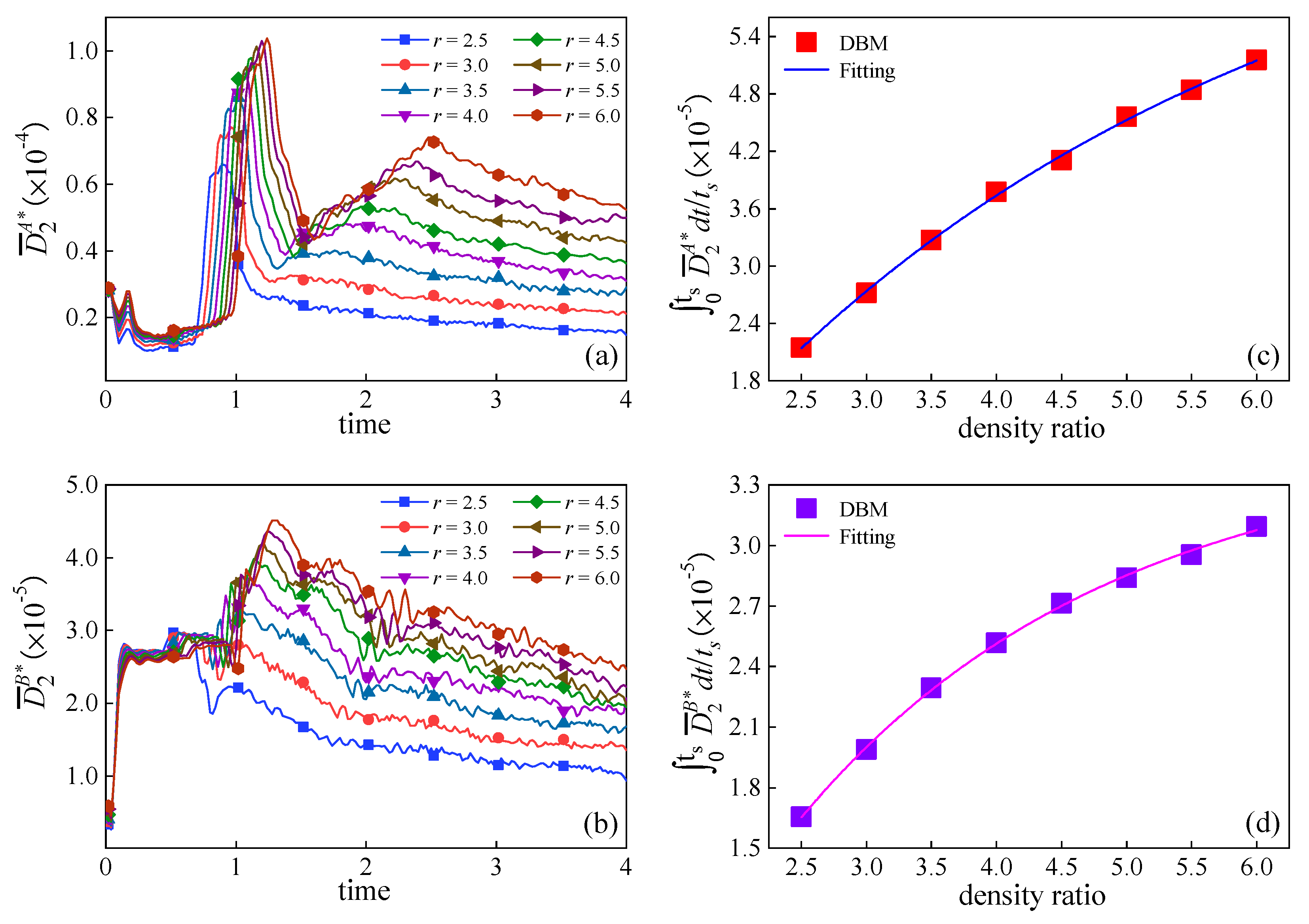
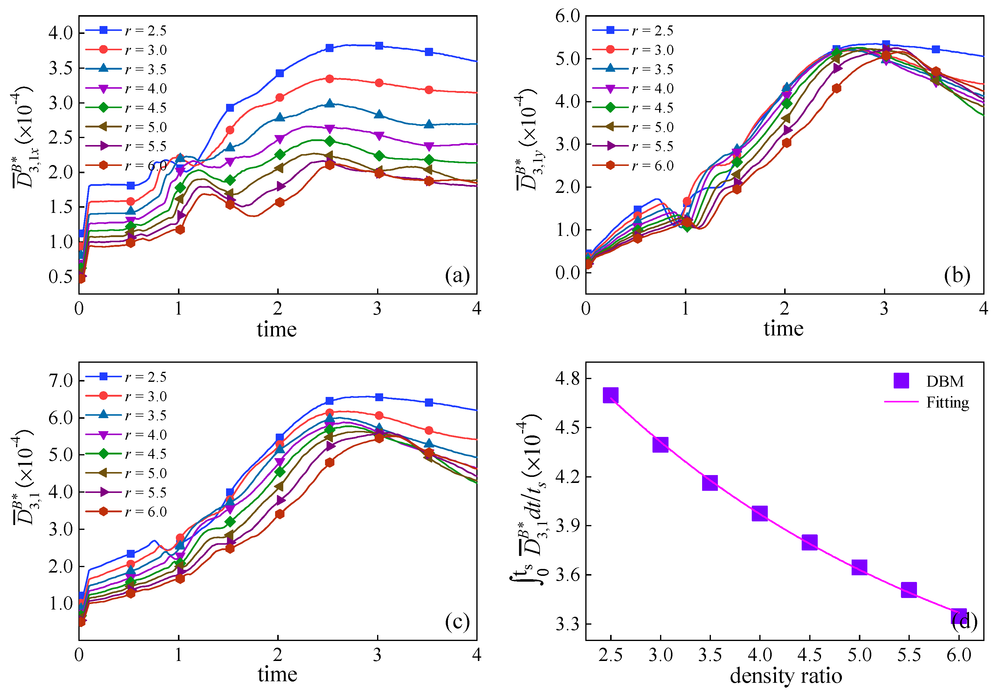
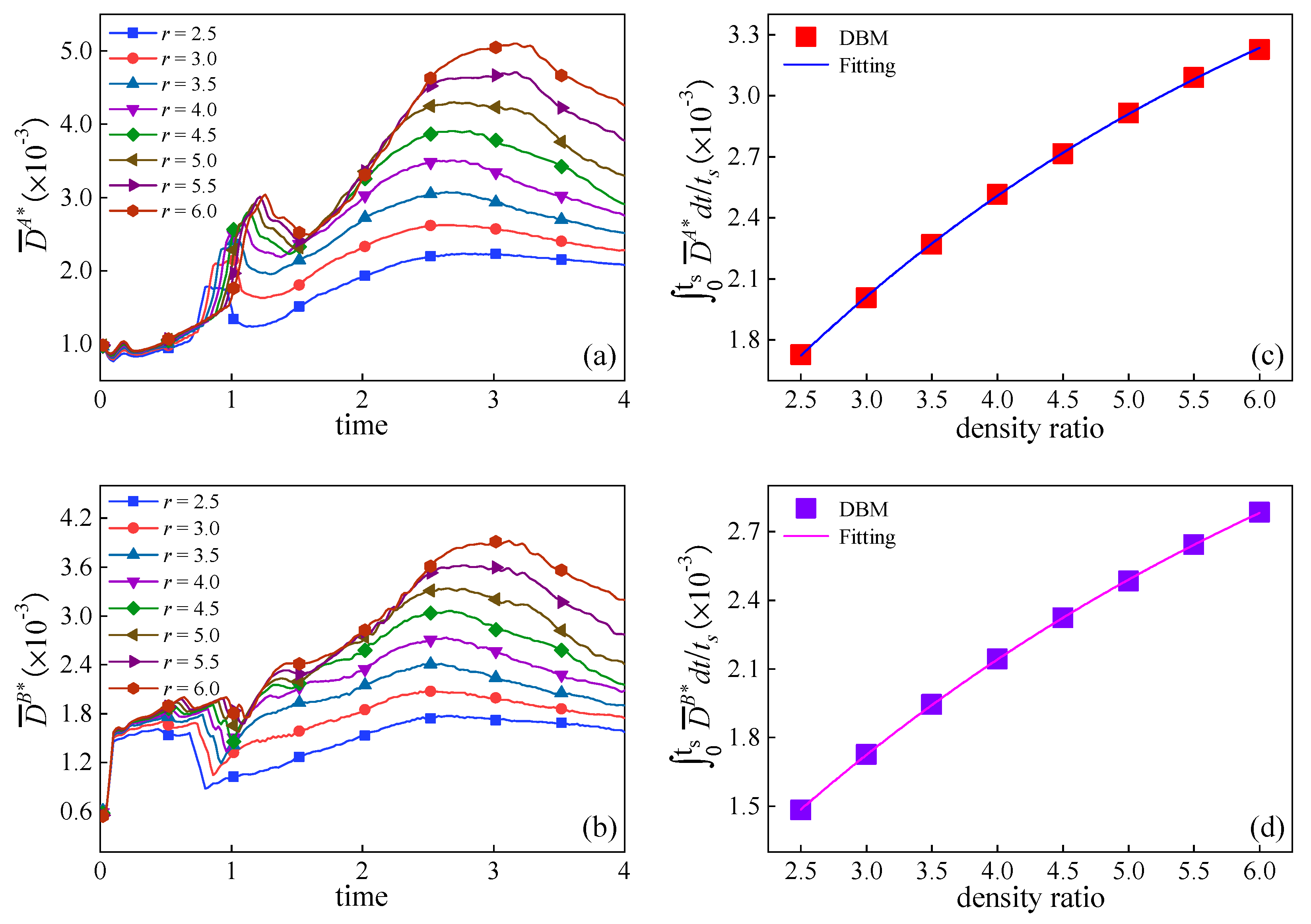
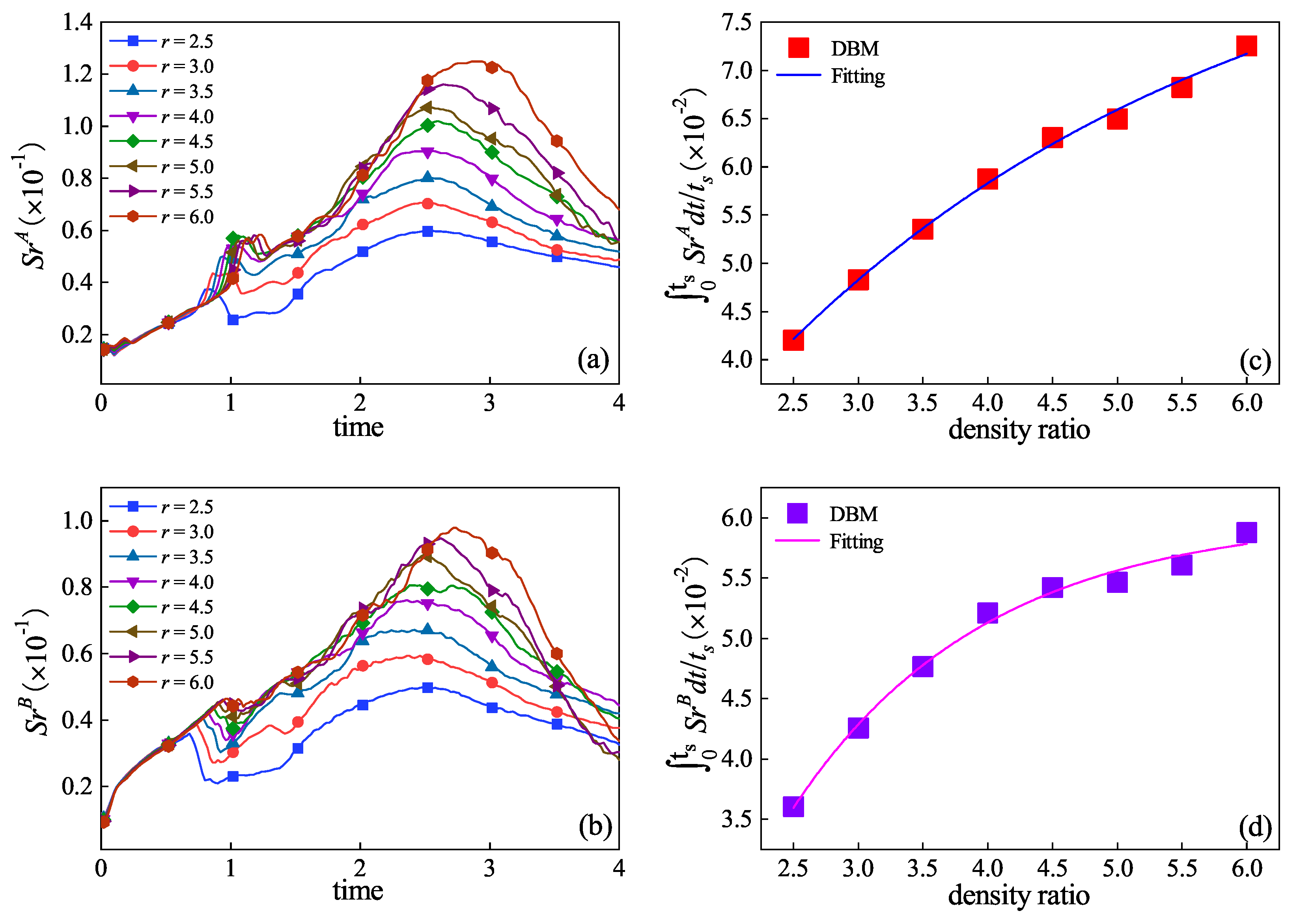
3.3. Thermodynamic Non-Equilibrium Effects

In this subsection, let us study the essential TNE behaviors in the process of the RM instability. First of all, the viscous stress tensor D ¯ 2 σ is explored in Figure 6. Subsequently, the average heat flux strength D ¯ 3 , 1 σ is investigated in Figure 7 and Figure 8. Then, the average TNE strength D ¯ σ is probed in Figure 9. Lastly, the proportion of the non-equilibrium region S r σ is discussed in Figure 10.
Figure 6a delineates the evolution of the viscous stress tensor D ¯ 2 A with different density ratios. It can be found that the whole level of D ¯ 2 A is higher for a larger density ratio. To better analyze the evolutionary mechanism of the RM instability, let us take r = 5.0 for example. Clearly, D ¯ 2 A decreases before t = 0.1 as the shock wave passes through the material interface. Then, D ¯ 2 A goes up during t = 0.1∼0.2 owing to the RM instability when the amplitude of the material interface rises. Subsequently, it goes down until about t = 0.4 because the reflected shock wave leaves the left boundary. Afterwards, there are few changes to D ¯ 2 A during 0.4 < t 0.9 while the RM instability has a weak effect on D ¯ 2 A . Later, at 0.9 < t 1.2 , D ¯ 2 A soars sharply because of the secondary impact of the reflected transmitted shock wave. During t = 1.2∼1.5, D ¯ 2 A decreases with the departure of the transmitted shock wave and transverse waves. After that, the material interface continues to develop after undergoing reversal, and the shear stress increases, causing D ¯ 2 A increases again. Ultimately ( t > 2.2 ), under the action of dissipation/diffusion, the vortex structure disappears and D ¯ 2 A decreases slowly.
The evolution of the viscous stress tensor D ¯ 2 B over time is depicted in Figure 6b. It can be found that the relationship between D ¯ 2 B and r changes in the process: (i) In the beginning, there is a positive correlation between D ¯ 2 B and r. This is correlated with the molecular mass of the initial setting, where the larger r corresponds to a greater molecular mass of component B, resulting in a greater D ¯ 2 B . (ii) Subsequently, D ¯ 2 B decreases as r increases during the stage of t = 0.1∼0.7, when the material interface moves rightwards and the transmitted shock wave propagates in the heavier medium filled with species B. With the increase in r, the density of component B increases, the flow velocity of the transmitted shock wave in component B falls, and, hence, the viscous stress is weakened. (iii) When t > 1.2 , D ¯ 2 B increases as r increases. During this stage, the reshock wave passes through the material interface, the heavy fluid flows into lighter fluid, the material interface evolution is accelerated, and D ¯ 2 B increases.
Additionally, the integration of D ¯ 2 σ (with σ = A , B) over time for various density ratios is described in Figure 6c,d. The fitting functions for the two species are expressed as 0 t s D ¯ 2 A d t / t s = [ 9.65 exp ( 0.24 r ) + 7.46 ] × 10 5 and 0 t s D ¯ 2 B d t / t s = [ 5.25 exp ( 0.42 r ) + 3.51 ] × 10 5 , respectively. Clearly, both D ¯ 2 A and D ¯ 2 B are positively correlated with r. It can be concluded that the larger the density ratio is, the faster the material interface evolves and the stronger the viscous stress becomes.
Next, we investigate the heat flux intensity in the RM process. Figure 7 exhibits the evolution of the heat flux intensities D ¯ 3 , 1 x A , D ¯ 3 , 1 y A , and D ¯ 3 , 1 A over time. It is observed in Figure 7a that D ¯ 3 , 1 x A shows a trend of increasing, afterward decreasing, then increasing, and finally decreasing overall in each case. Let us take the case of r = 5.0 for example. To be specific, the material interface is impacted by the shock wave before t = 0.1 and by the secondary shock wave during the phase of t = 0.9∼1.18. During the two stages, the mixing of two components accelerates, which promotes the heat exchange simultaneously, resulting in a rapid increase in D ¯ 3 , 1 x A . During the period t = 0.1∼0.5, the transmitted shock wave propagates into the heavier fluid and the change in D ¯ 3 , 1 x A is not obvious. For the phase of t = 0.5∼0.9, the transmitted shock wave is reflected back and moves leftwards, and D ¯ 3 , 1 x A rises gradually. Afterwards, as the transmitted shock wave departs from the physical system, the value of D ¯ 3 , 1 x A exhibits a downward trend. When t = 1.5∼2.3, D ¯ 3 , 1 x A increases because the vortex structure on the interface becomes more complex, the contact area of the fluid increases, and the heat exchange of the fluid system increases remarkably. After t = 2.3 , the two components are fully mixed, the fluid structure gradually disappears under the action of dissipation/diffusion, and D ¯ 3 , 1 x A shows a gradual declining trend.
Figure 7b shows the evolution of the heat flux intensity D ¯ 3 , 1 y A over time. It can be seen that for all cases, D ¯ 3 , 1 y A firstly rises, afterward falls, then increases, and eventually decreases. For the specific case of r = 5.0 , before t = 0.9 , the material interface is widened in the x direction continuously and the heat exchange in the y direction is enhanced due to the growth of the RM instability; hence, D ¯ 3 , 1 y A increases. During t = 0.9∼1.1, the reshock wave impacts the material interface; the material interface is compressed, resulting in a slight decrease in D ¯ 3 , 1 y A . Afterwards, as the RM instability evolves, the material interface is elongated constantly, the contact area between the two components increases, and the heat exchange is enhanced. Finally ( t > 3.0 ), under the action of dissipation and heat conduction, the fluid structure slowly disappears, the mixing degree of the two components is deeper, the physical field becomes smooth, and thereby, D ¯ 3 , 1 y A declines.
The evolution of the heat flux strength D ¯ 3 , 1 A of component A is depicted in Figure 7c. It is observed that D ¯ 3 , 1 A first shows a rising and then a falling tendency in each case on the whole. That is to say, the heat exchange of the system is elevated in the early stage and then diminished in the evolution of the RM instability. In fact, the variation of D ¯ 3 , 1 A in Figure 7c is consistent with the trends of D ¯ 3 , 1 x A in Figure 7a and D ¯ 3 , 1 y A in Figure 7b. To have a quantitative study, Figure 7d depicts the time integration of D ¯ 3 , 1 A versus the density ratio. The squares denote the numerical results and the line represents the fitting function 0 t s D ¯ 3 , 1 A d t / t s = [ 2.85 exp ( 0.18 r ) + 3.00 ] × 10 3 . It is evident that the larger the density ratio is, the faster the material interface evolves and the more significant the temperature gradient changes are.
Subsequently, the evolutions of the heat flux strengths D ¯ 3 , 1 x B , D ¯ 3 , 1 y B , and D ¯ 3 , 1 B for various density ratios are discussed: see Figure 8a–c. Their overall evolutionary trends are similar to that of component A. It is noteworthy that the heat flux strength of component B is negatively correlated with the density ratio. Specifically, for the heavier media, as r increases, the corresponding molecular mass becomes larger and the heat exchange of component B becomes weaker. It is further found that the relationship between 0 t s D ¯ 3 , 1 B d t / t s and r reads 0 t s D ¯ 3 , 1 B d t / t s = [ 4.21 exp ( 0.26 r ) + 2.49 ] × 10 4 . Obviously, with the increasing density ratio, D ¯ 3 , 1 x B decreases monotonically.
Next, to gain a deeper understanding of the TNE behavior in the RM instability system, the average TNE strength D ¯ σ is probed below. As seen in Figure 9a, for all examples, the profile of D ¯ A over time has a similar pattern and is positively related to the density ratio. Specifically, take r = 5.0 as an example. The TNE intensity of component A shows a fluctuating increase before t = 1.2 due to the impact of the shock wave on the material interface and the increase of the non-equilibrium area around the transmitted shock wave, reflected shock or rarefaction wave, and transverse waves. During t = 1.2∼1.5, the transverse waves and transmitted shock wave leave the computational domain, which causes a decrease in the physical gradient of the system. And when t > 1.5 , D ¯ A increases again and then decreases eventually. This phenomenon results from the competition between the following two mechanisms. On the one hand, the RM instability induced by the secondary impact continues to evolve, the width of the material interface increases, and the non-equilibrium region also increases: thereby, the TNE intensity is enhanced. On the other hand, under the dissipation/diffusion effect, the vortex structure gradually disappears and the physical field becomes smooth. The former (latter) plays a prominent role in the increase (decrease) stage.
In addition, Figure 9b shows the evolution of D ¯ B for various density ratios. For more detailed analysis of the evolution trend of D ¯ B , take r = 5 as an example. In the very early phase t < 0.1 , the shock wave rapidly passes through the material interface and enters the heavier medium. Sharp physical gradients start to emerge in the B medium, causing D ¯ B to surge rapidly. During the stage of t = 0.1∼0.9, D ¯ B rises with a small disturbance as the transmitted shock wave continues to propagate rightwards until it reaches the right boundary, at which point the transmitted shock wave is reflected and then propagates leftwards. Subsequently, the physical gradients decrease at t = 0.9∼1.1 as the transmitted shock wave passes through the material interface and leaves component B, and a reflected rarefaction wave is generated in the right region and then dissipates gradually. When t > 1.1 , it can be observed that D ¯ B shows a trend of increasing and then decreasing. The reason for the rise is that the material interface is reversed and elongated, the physical gradients change to become more complex, and the TNE is enhanced. Meanwhile, the decrease in the TNE strength D ¯ B results from the fact that the physical gradients become smooth under the effect of dissipation/diffusion.
Moreover, Figure 9c,d portray the relationship between the time integration of D ¯ σ and the density ratios. The fitting functions are 0 t s D ¯ A d t / t s = [ 4.91 exp ( 0.21 r ) + 4.62 ] × 10 3 and 0 t s D ¯ B d t / t s = [ 4.35 exp ( 0.18 r ) + 4.27 ] × 10 3 , where the integral is performed from t = 0 to t s = 4 . Physically, for a larger density ratio, the material interface becomes more complex and the increase to the physical gradient is larger, leading to the growth of the TNE intensity of each component.
Finally, for a more detailed description of the evolution law of the global TNE intensity, let us introduce the proportion of the non-equilibrium region S r σ , which is defined as the ratio of the non-equilibrium area to the total area of the fluid system [41]. Here, the non-equilibrium region is where the TNE intensity of species σ is greater than a threshold θ . In this work, the threshold value is chosen as θ = 0.02 .
Figure 10a shows that for any case, S r A firstly rises, afterwards falls, then rises again, and finally falls. Take r = 5.0 as an example: it can be seen that there is an increasing trend before t = 1.1 . The rise is attributed to the impact of the shock wave on the material interface as well as the increase in physical gradients near the transmitted shock wave, reflected shock or rarefaction wave, and transverse waves, enhancing the TNE intensity. From t = 1.1 to 1.3 , the TNE intensity is weakened as the transverse waves and transmitted shock wave depart the calculation region. During the period of t = 1.3∼2.5, the RM instability continues to evolve, the interface is continuously elongated, and the non-equilibrium region increases, and so S r A rises slowly. When t > 2.5 , the TNE intensity is decreased as the fine structure gradually disappears under the effect of dissipation/diffusion.
In the same way, Figure 10b describes the evolution of S r B for various density ratios r. The evolutionary trend of S r B is similar to that of S r A , and the physical mechanisms can be obtained by the analysis of S r A . Further, the time integration results of S r σ for various density ratios are depicted in Figure 10c,d. Their relationships are 0 t s S r A d t / t s = 0.10 exp ( 0.27 r ) + 0.09 and 0 t s S r B d t / t s = 0.12 exp ( 0.67 r ) + 0.06 , respectively. As a result, for a larger density ratio, the interface evolves faster and the macroscopic physical gradient changes are more significant, and thus, the TNE becomes stronger.

4. Conclusions

In this paper, the RM instability in the reshock process for various density ratios is investigated through the two-component DBM. Both hydrodynamic and TNE effects are analyzed in detail. On the whole, the average density gradients demonstrate a trend of rising, falling, rising again, and then falling eventually. A linearly increasing relationship is obtained between the time integration of the average density gradient and the density ratio. The main physical mechanisms are as follows. Firstly, the areas of density gradients are extended as the mixing of the two components accelerates under the action of the shock wave. Secondly, the global physical gradients decrease while the transmitted shock wave and transverse waves leave the calculational domain. Thirdly, the local macroscopic physical gradients decrease when the fluid structure gradually disappears due to dissipation/diffusion. Finally, the TNE effects are studied from various perspectives, including the average viscous stress tensor, heat flux intensity, TNE intensity, and proportion of the non-equilibrium region. It is found that the time integration of the TNE quantities and the proportion of the non-equilibrium region of each species are higher for a larger density ratio. However, the heat flux intensity of the heavier medium shows the opposite trend. Physically, there are several competitive mechanisms associated with these TNE quantities. (i) The TNE strength is significantly enhanced under the impact of the shock wave. (ii) The non-equilibrium region increases with the elongation of the material interface. (iii) The global non-equilibrium manifestation decreases as the transmitted shock wave and transverse waves leave or when the reflected rarefaction wave weakens. (iv) The global TNE intensity is enhanced (weakened) with an increase (decrease) in the macroscopic physical gradients. These findings can deepen our understanding of the RM instability with non-equilibrium effects during the reshock process from mesoscopic to macroscopic levels and are useful for understanding and mitigating the influence of hydrodynamic instabilities on indirect-drive ICF implosions [7,64,65,66]. Meanwhile, the research can also contribute to the knowledge of the interaction mechanism between shock waves and material interfaces, explosions, supersonic combustors [5,10], etc.

Author Contributions

Conceptualization, T.Y., C.L., H.L. and D.L.; methodology, T.Y., C.L., H.L. and D.L.; software, T.Y., C.L., H.L. and D.L.; validation, T.Y.; formal analysis, C.L., H.L. and D.L.; investigation, T.Y. and D.L.; resources, C.L. and H.L.; data curation, T.Y., C.L., H.L. and D.L.; writing—original draft preparation, T.Y.; writing—review and editing, T.Y., C.L., H.L. and D.L.; visualization, T.Y. and H.L.; supervision, C.L. and D.L.; project administration, C.L. and H.L.; funding acquisition, C.L. and H.L. All authors have read and agreed to the published version of the manuscript.

Funding

This work was supported by the National Natural Science Foundation of China (under grant Nos. U2242214, 51806116, and 11875001), the Natural Science Foundation of Fujian Province (under grant Nos. 2021J01652 and 2021J01655), and the Guangdong Basic and Applied Basic Research Foundation (under grant No. 2022A1515012116).

Data Availability Statement

The data used to support the findings of this study are available from the corresponding author upon request.

Conflicts of Interest

The authors declare no conflict of interest.

Nomenclature

σ chemical species
iindex of discrete velocity
f i σ ( f i σ e q ) discrete (equilibrium) distribution function
ttime
r space coordinate
v i discrete velocity
Ω i σ collision term
τ σ relaxation time
θ σ relaxation parameter
n σ , nnumber density
ρ σ , ρ mass density
u σ , u flow velocity
p σ , ppressure
m σ molecular mass
T σ , Ttemperature
E σ , Einternal energy density
Dspatial dimension
Iextra degrees of freedom
C an N × N matrix
C 1 the inverse matrix of C
M m , n σ ( f i σ e q ) central kinetic moments of f i σ e q
M m , n σ ( f i σ ) central kinetic moments of f i σ
v i peculiar velocity
Δ 2 σ non-organized momentum flux
Δ 3 , 1 σ non-organized energy flux
Δ 3 σ flux of non-organized momentum flux
Δ 4 , 2 σ flux of non-organized energy flux
Δ σ                total thermodynamic non-equilibrium quantity
D ¯ 2 σ average of Δ 2 σ over the physical system
D ¯ 3 , 1 σ average of Δ 3 , 1 σ over the physical system
D ¯ 3 σ average of Δ 3 σ over the physical system
D ¯ 4 , 2 σ average of Δ 4 , 2 σ over the physical system
D ¯ σ average of Δ σ over the physical system
L x length of the fluid system
L y width of the fluid system
v a , v b , v c , v d size of discrete velocities
η a , η b , η c , η d parameter of extra degrees of freedom
L, M, Rleft, middle, and right regions
Ma Mach number
A 0 perturbation amplitude
kwave number
rdensity ratio
A t Atwood number
N x , N y mesh grids
Δ x , Δ y space step
Δ t time step
vamplitude growth
A 1 post-shock Atwood number
a 0 post-shock amplitude
Δ u the change of interface velocity
ω vorticity
ρ ¯ average density gradient over the physical system
x ρ ¯ average density gradient in the x direction over the physical system
y ρ ¯ average density gradient in the y direction over the physical system
γ specific heat ratio
κ heat conductivity
μ σ dynamic viscosity coefficient
einternal energy of the mixing system per unit mass

Appendix A. Navier–Stokes Equations

Via Chapman–Enskog expansion, the DBM can recover the following Navier–Stokes equations in the continuum limit:
ρ t + r α ρ u α = 0 ,
t ρ u α + r β σ δ α β p σ + ρ σ u α σ u β σ + r β σ P α β σ = 0 ,
t ρ e + 1 2 u 2 + r α σ ρ σ u α σ e σ + 1 2 u σ 2 + p σ u α σ r α σ κ σ r α D + I 2 T σ m σ u β σ P α β σ + Y α σ = 0 ,
with
P α β σ = μ σ u α σ r β + u β σ r α 2 δ α β D + I u χ σ r χ ,
Y α σ = ρ σ u α σ D + I u β σ u β 2 ρ σ u α σ u α 2 D + I + 2 m σ T σ T + u σ 2 u 2 ,
where p σ = n σ T σ , e σ = ( D + I ) T σ / ( 2 m σ ) , μ σ = p σ τ σ , κ = γ μ σ , γ = ( D + I + 2 ) / ( D + I ) , and e = σ ρ σ ( e σ + u σ 2 / 2 ) / ρ u 2 / 2 denote the pressure, internal energy per unit mass, dynamic viscosity coefficient, heat conductivity, specific heat ratio, and internal energy of the mixing system per unit mass, respectively. The term δ α β represents the Kronecker function, and the subscripts α , β , χ stand for x or y.

Appendix B. Expressions of the Kinetic Moments

The equilibrium distribution function f i σ e q satisfies the following seven kinetic moments:
M 0 f i σ e q = i f i σ e q = i f i σ = n σ ,
M 1 f i σ e q = i f i σ e q v i = i f i σ v i = n σ u ,
M 2 , 0 f i σ e q = i f i σ e q ( v i · v i + η i 2 ) = i f i σ ( v i · v i + η i 2 ) = n σ ( D + I ) T m σ + u · u ,
M 2 f i σ e q = i f i σ e q v i v i = n σ T m σ e α e β δ α β + u · u ,
M 3 , 1 f i σ e q = i f i σ e q ( v i · v i + η i 2 ) v i = n σ u ( D + I + 2 ) T m σ + u · u ) ,
M 3 f i σ e q = i f i σ e q v i v i v i = n σ T m σ u α e β e χ δ β χ + u β e α e χ δ α χ + u χ e α e β δ α β + u u u ,
M 4 , 2 f i σ e q = i f i σ e q ( v i · v i + η i 2 ) v i v i = n σ T m σ [ ( D + I + 2 ) T m σ + u · u ] e α e β δ α β + n σ u u ( D + I + 4 ) T m σ + u · u ] .

Appendix C. The Verification of Grid Convergence

To ensure an accurate and effective simulation of the RM instability, the grid independence is verified. Figure A1 depicts the profile of the density along the center line L y / 2 in the case of r = 2.5 at the time instant t = 2.0 . We choose four different grid sizes: N x × N y = 250 × 50 , 500 × 100 , 1000 × 200 , and 2000 × 400 . It can be found that the simulation results gradually converge as the number of mesh grids increases. To be specific, the simulation results for 1000 × 200 and 2000 × 400 are close to each other. This means that the simulation accuracy is high enough for 2000 × 400 . Consequently, a grid size of N x × N y = 2000 × 400 with a corresponding spatial step of Δ x = Δ y = 2.5 × 10 4 is adopted for all simulations in this paper.
Figure A1. The verification of grid convergence: the density profiles are plotted along the center line L y / 2 at the time instant t = 2.0 for the RM process.
Inventions 08 00157 g0a1

References

  1. Richtmyer, R.D. Taylor instability in shock acceleration of compressible fluids. Commun. Pur. Appl. Math. 1960, 13, 297–317. [Google Scholar] [CrossRef]
  2. Meshkov, E. Instability of the interface of two gases accelerated by a shock wave. Fluid Dynam. 1969, 4, 101–104. [Google Scholar] [CrossRef]
  3. Brouillette, M. The Richtmyer-Meshkov instability. Annu. Rev. Fluid Mech. 2002, 34, 445–468. [Google Scholar] [CrossRef]
  4. Poludnenko, A.Y.; Chambers, J.; Ahmed, K.; Gamezo, V.N.; Taylor, B.D. A unified mechanism for unconfined deflagration-to-detonation transition in terrestrial chemical systems and type Ia supernovae. Science 2019, 366, eaau7365. [Google Scholar] [CrossRef] [PubMed]
  5. Morris, C.; Hopson, J.W.; Goldstone, P. Proton radiography. Los Alamos Sci. 2006, 30, 32. [Google Scholar]
  6. Yang, J.; Kubota, T.; Zukoski, E.E. A model for characterization of a vortex pair formed by shock passage over a light-gas inhomogeneity. J. Fluid Mech. 1994, 258, 217–244. [Google Scholar] [CrossRef]
  7. MacPhee, A.; Smalyuk, V.; Landen, O.; Weber, C.; Robey, H.; Alfonso, E.; Baker, K.; Berzak, H.L.; Biener, J.; Bunn, T.; et al. Hydrodynamic instabilities seeded by the X-ray shadow of ICF capsule fill-tubes. Phys. Plasmas 2018, 25, 082702. [Google Scholar] [CrossRef]
  8. Roycroft, R.; Sauppe, J.P.; Bradley, P.A. Double cylinder target design for study of hydrodynamic instabilities in multi-shell ICF. Phys. Plasmas 2022, 29, 032704. [Google Scholar] [CrossRef]
  9. Mostert, W.; Wheatley, V.; Samtaney, R.; Pullin, D.I. Effects of magnetic fields on magnetohydrodynamic cylindrical and spherica Richtmyer-Meshkov instability. Phys. Fluids 2015, 27, 104102. [Google Scholar] [CrossRef]
  10. Attal, N.; Ramaprabhu, P. Numerical investigation of a single-mode chemically reacting Richtmyer-Meshkov instability. Shock Waves 2015, 25, 307–328. [Google Scholar] [CrossRef]
  11. Valerio, E.; Jourdan, G.; Houas, L.; Zeitoun, D.; Besnard, D. Modeling of Richtmyer-Meshkov instability-induced turbulent mixing in shock-tube experiments. Phys. Fluids 1999, 11, 214–225. [Google Scholar] [CrossRef]
  12. Guo, X.; Si, T.; Zhai, Z.; Luo, X. Large-amplitude effects on interface perturbation growth in Richtmyer-Meshkov flows with reshock. Phys. Fluids 2022, 34, 082118. [Google Scholar] [CrossRef]
  13. Cong, Z.; Guo, X.; Si, T.; Luo, X. Experimental and theoretical studies on heavy fluid layers with reshock. Phys. Fluids 2022, 34, 104108. [Google Scholar] [CrossRef]
  14. Wang, H.; Ding, J.; Si, T.; Luo, X. Richtmyer-Meshkov instability of a single-mode interface with reshock. Acta Aerodyn. Sin. 2022, 40, 33–40. [Google Scholar]
  15. Guo, X.; Cong, Z.; Si, T.; Luo, X. Shock-tube studies of single-and quasi-single-mode perturbation growth in Richtmyer-Meshkov flows with reshock. J. Fluid Mech. 2022, 941, 65. [Google Scholar] [CrossRef]
  16. Nagel, S.; Raman, K.; Huntington, C.; MacLaren, S.; Wang, P.; Bender, J.; Prisbrey, S.; Zhou, Y. Experiments on the single-mode Richtmyer-Meshkov instability with reshock at high energy densities. Phys. Plasmas 2022, 29, 032308. [Google Scholar] [CrossRef]
  17. Rasteiro Dos Santos, M.; Bury, Y.; Jamme, S.; Griffond, J. On the effect of characterised initial conditions on the evolution of the mixing induced by the richtmyer–meshkov instability. Shock Waves 2023, 33, 117–130. [Google Scholar] [CrossRef]
  18. Ukai, S.; Balakrishnan, K.; Menon, S. Growth rate predictions of single-and multi-mode Richtmyer-Meshkov instability with reshock. Shock Waves 2011, 21, 533–546. [Google Scholar] [CrossRef]
  19. Tritschler, V.K.; Olson, B.J.; Lele, S.K.; Hickel, S.; Hu, X.; Adams, N.A. On the Richtmyer-Meshkov instability evolving from a deterministic multimode planar interface. J. Fluid Mech. 2014, 755, 429–462. [Google Scholar] [CrossRef]
  20. Olson, B.J.; Greenough, J.A. Comparison of two-and three-dimensional simulations of miscible Richtmyer-Meshkov instability with multimode initial conditions. Phys. Fluids 2014, 26, 101702. [Google Scholar] [CrossRef]
  21. Li, H.; He, Z.; Zhang, Y.; Tian, B. On the role of rarefaction/compression waves in Richtmyer-Meshkov instability with reshock. Phys. Fluids 2019, 31, 054102. [Google Scholar] [CrossRef]
  22. Latini, M.; Schilling, O. A comparison of two-and three-dimensional single-mode reshocked Richtmyer-Meshkov instability growth. Physica D 2020, 401, 132201. [Google Scholar] [CrossRef]
  23. Bin, Y.; Xiao, M.; Shi, Y.; Zhang, Y.; Chen, S. A new idea to predict reshocked Richtmyer-Meshkov mixing: Constrained large-eddy simulation. J. Fluid Mech. 2021, 918, R1. [Google Scholar] [CrossRef]
  24. Mohaghar, M.; McFarland, J.; Ranjan, D. Three-dimensional simulations of reshocked inclined Richtmyer-Meshkov instability: Effects of initial perturbations. Phys. Rev. Fluids 2022, 7, 093902. [Google Scholar] [CrossRef]
  25. Wu, Z.; Huang, S.; Ding, J.; Wang, W.; Luo, X. Molecular dynamics simulation of cylindrical Richtmyer-Meshkov instability. Sci. Chin. Phys. Mech. Astron. 2018, 61, 114712. [Google Scholar] [CrossRef]
  26. Liu, H.; Yu, B.; Chen, H.; Chen, H.; Zhang, B.; Xu, H.; Liu, H. Contribution of viscosity to the circulation deposition in the Richtmyer–Meshkov instability. J. Fluid Mech. 2020, 895, A10. [Google Scholar] [CrossRef]
  27. Lin, C.; Xu, A.; Zhang, G.; Li, Y.; Succi, S. Polar-coordinate lattice Boltzmann modeling of compressible flows. Phys. Rev. E 2014, 89, 013307. [Google Scholar] [CrossRef] [PubMed]
  28. Chen, F.; Xu, A.; Zhang, G. Collaboration and competition between Richtmyer-Meshkov instability and Rayleigh-Taylor instability. Phys. Fluids 2018, 30, 102105. [Google Scholar] [CrossRef]
  29. Shan, Y.; Xu, A.; Wang, L.; Zhang, Y. Nonequilibrium kinetics effects in Richtmyer–Meshkov instability and reshock processes. Commun. Theor. Phys. 2023, 75, 115601. [Google Scholar] [CrossRef]
  30. Xu, A.; Zhang, G.; Gan, Y.; Chen, F.; Yu, X. Lattice Boltzmann modeling and simulation of compressible flows. Front. Phys. 2012, 7, 582–600. [Google Scholar] [CrossRef]
  31. Xu, A.; Shan, Y.; Chen, F.; Gan, Y.; Lin, C. Progress of mesoscale modeling and investigation of combustion multiphase flow. Acta Aero. Astro. Sin. 2021, 42, 625842. [Google Scholar]
  32. Benzi, R.; Succi, S.; Vergassola, M. The lattice Boltzmann equation: Theory and applications. Phys. Rep. 1992, 222, 145–197. [Google Scholar] [CrossRef]
  33. Wei, Y.; Yang, H.; Dou, H.; Lin, Z.; Wang, Z.; Qian, Y. A novel two-dimensional coupled lattice Boltzmann model for thermal incompressible flows. Appl. Math. Comput. 2018, 339, 556–567. [Google Scholar] [CrossRef]
  34. Wang, Z.; Wei, Y.; Qian, Y. A bounce back-immersed boundary-lattice Boltzmann model for curved boundary. Appl. Math. Model. 2020, 81, 428–440. [Google Scholar] [CrossRef]
  35. Wang, Z.; Wei, Y.; Qian, Y. A novel thermal lattice Boltzmann model with heat source and its application in incompressible flow. Appl. Math. Model. 2022, 427, 127167. [Google Scholar] [CrossRef]
  36. Li, Q.; Jiang, J.; Hong, Y.; Du, J. Numerical investigation of thermal management performances in a solar photovoltaic system by using the phase change material coupled with bifurcated fractal fins. J. Energy Storage 2022, 56, 106156. [Google Scholar] [CrossRef]
  37. Fei, L.; Qin, F.; Zhao, J.; Derome, D.; Carmeliet, J. Lattice boltzmann modelling of isothermal two-component evaporation in porous media. J. Fluid Mec. 2023, 955, 18. [Google Scholar] [CrossRef]
  38. Li, Q.; Xing, Y.; Huang, R. Equations of state in multiphase lattice Boltzmann method revisited. Phys. Rev. E 2023, 107, 015301. [Google Scholar] [CrossRef]
  39. Lai, H.; Xu, A.; Zhang, G.; Gan, Y.; Ying, Y.; Succi, S. Nonequilibrium thermohydrodynamic effects on the Rayleigh-Taylor instability in compressible flows. Phys. Rev. E 2016, 94, 023106. [Google Scholar] [CrossRef]
  40. Lin, C.; Luo, K.; Xu, A.; Gan, Y.; Lai, H. Multiple-relaxation-time discrete Boltzmann modeling of multicomponent mixture with nonequilibrium effects. Phys. Rev. E 2021, 103, 013305. [Google Scholar] [CrossRef]
  41. Chen, L.; Lai, H.; Lin, C.; Li, D. Specific heat ratio effects of compressible Rayleigh-Taylor instability studied by discrete Boltzmann method. Front. Phys. 2021, 16, 52500. [Google Scholar] [CrossRef]
  42. Li, Y.; Lai, H.; Lin, C.; Li, D. Influence of the tangential velocity on the compressible Kelvin-Helmholtz instability with nonequilibrium effects. Front. Phys. 2022, 17, 63500. [Google Scholar] [CrossRef]
  43. Zhang, D.; Xu, A.; Song, J.; Gan, Y.; Zhang, Y.; Li, Y. Specific-heat ratio effects on the interaction between shock wave and heavy-cylindrical bubble: Based on discrete Boltzmann method. arXiv 2023, arXiv:2302.05687. [Google Scholar] [CrossRef]
  44. Gan, Y.; Xu, A.; Zhang, G.; Succi, S. Discrete Boltzmann modeling of multiphase flows: Hydrodynamic and thermodynamic non-equilibrium effects. Soft Matter 2015, 11, 5336–5345. [Google Scholar] [CrossRef] [PubMed]
  45. Gan, Y.; Xu, A.; Lai, H.; Li, W.; Sun, G.; Succi, S. Discrete Boltzmann multi-scale modelling of non-equilibrium multiphase flows. J. Fluid Mech. 2022, 951, A8. [Google Scholar] [CrossRef]
  46. Lin, C.; Luo, K. Discrete Boltzmann modeling of unsteady reactive flows with nonequilibrium effects. Phys. Rev. E 2019, 99, 012142. [Google Scholar] [CrossRef] [PubMed]
  47. Lombardini, M.; Hill, D.; Pullin, D.; Meiron, D. Atwood ratio dependence of Richtmyer-Meshkov flows under reshock conditions using large-eddy simulations. J. Fluid Mech. 2011, 670, 439–480. [Google Scholar] [CrossRef]
  48. Zhou, Y.; Cabot, W.H.; Thornber, B. Asymptotic behavior of the mixed mass in Rayleigh-Taylor and Richtmyer-Meshkov instability induced flows. Phys. Plasmas 2016, 23, 052712. [Google Scholar] [CrossRef]
  49. Chen, Q.; Li, L.; Zhang, Y.; Tian, B. Effects of the Atwood number on the Richtmyer-Meshkov instability in elastic-plastic media. Phys. Rev. E 2019, 99, 053102. [Google Scholar] [CrossRef]
  50. Liao, S.; Zhang, W.; Chen, H.; Zou, L.; Liu, J.; Zheng, X. Atwood number effects on the instability of a uniform interface driven by a perturbed shockwave. Phys. Rev. E 2019, 99, 013103. [Google Scholar] [CrossRef]
  51. Tang, J.; Zhang, F.; Luo, X.; Zhai, Z. Effect of Atwood number on convergent Richtmyer-Meshkov instability. Acta Mech. Sin. 2021, 37, 434–446. [Google Scholar] [CrossRef]
  52. Ren, J.; Culp, D.; Smith, B.; Ma, X. An investigation of the multi-mode Richtmyer-Meshkov instability at a gas/HE interface using Pagosa. Comput. Math. Appl. 2022, 139, 136–151. [Google Scholar] [CrossRef]
  53. Lin, C.; Xu, A.; Zhang, G.; Li, Y. Double-distribution-function discrete Boltzmann model for combustion. Combust. Flame 2016, 164, 137–151. [Google Scholar] [CrossRef]
  54. Zhang, H.; Zhuang, F. NND schemes and their applications to numerical simulation of two-and three-dimensional flows. Adv. Appl. Mech. 1991, 29, 193–256. [Google Scholar]
  55. Lin, C.; Luo, K. Mesoscopic simulation of nonequilibrium detonation with discrete boltzmann method. Combust. Flame 2018, 198, 356–362. [Google Scholar] [CrossRef]
  56. Succi, S. The Lattice Boltzmann Equation: For Fluid Dynamics and Beyond; Oxford University Press: Oxford, UK, 1992. [Google Scholar]
  57. Mohamad, A. Lattice Boltzmann Method; Springer: London, UK, 2001. [Google Scholar]
  58. Guo, Z.; Shu, C. Lattice Boltzmann Method and Its Application Inengineering; World Scientific: Singapore, 2013. [Google Scholar]
  59. Gan, Y.; Xu, A.; Zhang, G.; Li, Y. Lattice Boltzmann study on Kelvin-Helmholtz instability: Roles of velocity and density gradients. Phys. Rev. E 2011, 83, 056704. [Google Scholar] [CrossRef] [PubMed]
  60. Zel’Dovich, Y.B.; Raizer, Y.P. Physics of Shock Waves and High-Temperature Hydrodynamic Phenomena; Publisher Courier Corporation: North Chelmsford, MA, USA, 2002. [Google Scholar]
  61. Zhang, Q.; Sohn, S.-I. Padé approximation to an interfacial fluid mixing problem. Appl. Math. Lett. 1997, 10, 121–127. [Google Scholar] [CrossRef]
  62. Frahan, M.T.H.; Movahed, P.; Johnsen, E. Numerical simulations of a shock interacting with successive interfaces using the discontinuous Galerkin method: The multilayered Richtmyer-Meshkov and Rayleigh-Taylor instabilities. Shock Waves 2015, 25, 329–345. [Google Scholar] [CrossRef]
  63. Jourdan, G.; Houas, L. High-amplitude single-mode perturbation evolution at the Richtmyer-Meshkov instability. Phys. Rev. Lett. 2005, 95, 204502. [Google Scholar] [CrossRef]
  64. Craxton, R.S.; Anderson, K.S.; Boehly, T.R.; Goncharov, V.N.; Harding, D.R.; Knauer, J.P.; McCrory, R.L.; McKenty, P.W.; Meyerhofer, D.D.; Myatt, J.F.; et al. Direct-drive inertial confinement fusion: A review. Phys. Plasmas 2015, 22, 110501. [Google Scholar] [CrossRef]
  65. Wright, C.E.; Abarzhi, S.I. Effect of adiabatic index on Richtmyer-Meshkov flows induced by strong shocks. Phys. Fluids 2021, 33, 046109. [Google Scholar] [CrossRef]
  66. Lindl, J.D.; Amendt, P.; Berger, R.L.; Glendinning, S.G.; Glenzer, S.H.; Haan, S.W.; Kauffman, R.L.; Landen, O.L.; Suter, L.J. The physics basis for ignition using indirect-drive targets on the National Ignition Facility. Phys. Plasmas 2004, 11, 339–491. [Google Scholar] [CrossRef]
Figure 1. The initial configuration of the RM instability.
Inventions 08 00157 g001
Figure 2. Comparison of the growth rates of the RM instabilities given by the DBM and the Zhang–Sohn model [61].
Inventions 08 00157 g002
Figure 3. The first to third columns show contours of the density, non-equilibrium strength and vorticity in the RM process in the case of r = 2.5 , respectively.
Inventions 08 00157 g003
Figure 4. The first to third columns show contours of the density, non-equilibrium strength, and vorticity, respectively, for the RM process in the case of r = 5.0 .
Inventions 08 00157 g004
Figure 5. (a) Average density gradient in the x direction versus time. (b) Average density gradient in the y direction versus time. (c) Average density gradient versus time. (d) 0 t s | x ρ ¯ | d t / t s versus density ratios. (e) 0 t s | y ρ ¯ | d t / t s versus density ratios. (f) 0 t s | ρ ¯ | d t / t s versus density ratios.
Inventions 08 00157 g005
Figure 6. (a) Viscous stress tensor of component A versus time. (b) Viscous stress tensor of component B versus time. (c) 0 t s D ¯ 2 A d t / t s versus density ratios. (d) 0 t s D ¯ 2 B d t / t s versus density ratios.
Inventions 08 00157 g006
Figure 7. Average heat flux strength D ¯ 3 , 1 x A (a), D ¯ 3 , 1 y A (b), and D ¯ 3 , 1 A (c) of component A versus time. (d) 0 t s D ¯ 3 , 1 A d t / t s versus density ratios.
Inventions 08 00157 g007
Figure 8. Average heat flux strength D ¯ 3 , 1 x B (a), D ¯ 3 , 1 y B (b), and D ¯ 3 , 1 B (c) of component B versus time. (d) 0 t s D ¯ 3 , 1 B d t / t s versus density ratios.
Inventions 08 00157 g008
Figure 9. (a) Average TNE strength of component A versus time. (b) Average TNE strength of component B versus time. (c) 0 t s D ¯ A d t / t s versus density ratios. (d) 0 t s D ¯ B d t / t s versus density ratios.
Inventions 08 00157 g009
Figure 10. (a) The proportion of the non-equilibrium region of component A versus time. (b) The proportion of the non-equilibrium region of component B versus time. (c) 0 t s S r A d t / t s versus density ratios. (d) 0 t s S r B d t / t s versus density ratios.
Inventions 08 00157 g010
Disclaimer/Publisher’s Note: The statements, opinions and data contained in all publications are solely those of the individual author(s) and contributor(s) and not of MDPI and/or the editor(s). MDPI and/or the editor(s) disclaim responsibility for any injury to people or property resulting from any ideas, methods, instructions or products referred to in the content.

