Abstract
It is crucial for both traffic management organisations and individual commuters to be able to forecast traffic flows accurately. Graph neural networks made great strides in this field owing to their exceptional capacity to capture spatial correlations. However, existing approaches predominantly focus on local geographic correlations, ignoring cross-region interdependencies in a global context, which is insufficient to extract comprehensive semantic relationships, thereby limiting prediction accuracy. Additionally, most GCN-based models rely on pre-defined graphs and unchanging adjacency matrices to reflect the spatial relationships among node features, neglecting the dynamics of spatio-temporal features and leading to challenges in capturing the complexity and dynamic spatial dependencies in traffic data. To tackle these issues, this paper puts forward a fresh approach: a new self-supervised dynamic spatio-temporal graph convolutional network (SDSC) for traffic flow forecasting. The proposed SDSC model is a hierarchically structured graph–neural architecture that is intended to augment the representation of dynamic traffic patterns through a self-supervised learning paradigm. Specifically, a dynamic graph is created using a combination of temporal, spatial, and traffic data; then, a regional graph is constructed based on geographic correlation using clustering to capture cross-regional interdependencies. In the feature learning module, spatio-temporal correlations in traffic data are subjected to recursive extraction using dynamic graph convolution facilitated by Recurrent Neural Networks (RNNs). Furthermore, self-supervised learning is embedded within the network training process as an auxiliary task, with the objective of enhancing the prediction task by optimising the mutual information of the learned features across the two graph networks. The superior performance of the proposed SDSC model in comparison with SOTA approaches was confirmed by comprehensive experiments conducted on real road datasets, PeMSD4 and PeMSD8. These findings validate the efficacy of dynamic graph modelling and self-supervision tasks in improving the precision of traffic flow prediction.
1. Introduction
With the accelerated process of urbanisation and the increase in the number of vehicles, urban areas are facing increasing transport challenges such as traffic congestion, increased energy consumption, and environmental pollution, which have seriously affected the quality of people’s daily mobility. The “2021 Beijing Commuting Characteristics Annual Report” by the Beijing Institute of Transportation Development highlights that in 2021, the average commuting time in central Beijing was 51 min. Particularly, areas like Beijing Station and Jinsong experienced severe congestion totalling over 200 min during morning peak hours in May. These phenomena not only highlight the pressures on urban traffic management but also the importance of optimising traffic flow. Accurate traffic flow forecasting can help city managers develop more effective transport planning strategies, which can reduce energy consumption, mitigate environmental pollution, and improve the quality of life and well-being of residents.
Traffic flow prediction is usually trained on historical traffic data (including vehicle flow, speed, road conditions, and other information) to predict the future traffic flow on a particular road section or area. Current traffic flow prediction methods can be broadly classified into traditional methods and deep learning-based methods. Although traditional methods, such as historical averaging models [1], Autoregressive Integral Moving Average (ARIMA) [2], Support Vector Machines [3], and K Nearest Neighbours (KNNs) [4], can provide more reasonable prediction results in some static environments, it is usually difficult to adequately capture the spatial and temporal dynamics of traffic flow when faced with complex and changing urban traffic networks.
In contrast, deep learning-based models have shown some advantages in dealing with spatio-temporal variations in traffic flow. For example, convolutional neural networks (CNNs) [5] are able to deal efficiently with local spatial features, Long Short-Term Memory Networks (LSTMs) [6] excel at capturing long-term temporal dependencies, attention mechanisms [7] enhance the focus on information at critical moments, and temporal convolutional networks (TCNs) [8,9] capture long-term dependencies by expanding the sensory field. These deep learning methods have significantly improved prediction accuracy in many applications. However, they still face many challenges in dealing with cross-region dependencies and rapid dynamic changes in traffic networks. While LSTMs and TCNs perform well in capturing complex temporal dependencies, they have limitations in dealing with complex spatial relationships among multiple regions. Meanwhile, CNNs may also be insufficient in extracting global features in traffic networks to capture the full dynamic changes among different regions.
To cope with the dynamic changes in complex traffic networks, researchers have gradually introduced graph convolutional networks (GCNs) [10] to model traffic networks. GCNs are able to capture the spatial correlation between nodes (e.g., intersections or endpoints of roads) and edges (the connectivity between them) in a traffic network effectively by connecting them through a graph structure. Through this modelling approach, a GCN is highly expressive in dealing with dynamic traffic flows and interactions among complex regions. For example, the VSTGC model [11] uses a GCN to capture spatial correlation in traffic networks and incorporates temporal convolution to capture temporal dependence, which significantly improves prediction accuracy, while the GTDMGCN model [12] achieves excellent results in modelling complex traffic networks by adopting a multi-graph structure rather than a single-graph structure. The authors of [13,14] combine the advantages of temporal convolutional networks (TCNs) and graph convolutional networks (GCNs) to propose improved models that perform well in traffic flow prediction tasks. Specifically, the model in [13] uses an improved TCN to extract temporal and local spatial features, while a GCN is used to capture the topological relationships among road nodes, which achieves an effective fusion of temporal and spatial features. On the other hand, the model in [14] proposes a TCN-STGCN framework, which consists of spectral domain graph convolution and an improved TCN. The graph convolution part extracts the spatial dimensional information, while the temporal convolution part enhances the temporal sensory field by diffusion convolution. This improved framework effectively integrates the advantages of temporal convolution and graph convolution to improve the accuracy of traffic flow prediction.
Although these GCN-based models have made significant progress in modelling spatial features, they still suffer from a number of shortcomings when dealing with high-speed dynamic changes and the diversity of complex traffic patterns. First, traditional GCN models are usually based on static graph structures, which limits their adaptability in highly dynamic environments. For example, when unexpected events or traffic patterns change rapidly, the fixed graph structure may not be able to adapt in a timely manner, leading to insufficient capture of new dynamic dependencies by the model, which affects the accuracy of the prediction. In addition, since the convolution operation of GCNs mainly focuses on local nodes and their neighbouring nodes, the information on inter-regional dependencies gradually decays during the propagation process, resulting in the poor performance of the model in capturing the dependencies among long-distance regions. This limitation makes it difficult for GCNs to exploit important information fully among functionally related but spatially distant regions.
To overcome these limitations, researchers have introduced the attention mechanism into GCN models. The attention mechanism allows the model to adjust its attention dynamically to different time points and spatial locations, thus capturing complex spatio-temporal relationships more flexibly and accurately. However, existing models still face some challenges in dealing with the inter-regional dependencies and spatio-temporal dynamics of complex traffic flows. For example, although the ASTGCN [15] model captures dynamic correlations in traffic data through a spatio-temporal attention mechanism, because of its reliance on a static graph structure and a fixed time window, the model may not be able to adjust its attention in a timely manner in the face of rapid changes and unexpected events, thus affecting the prediction accuracy. The AMGCRN [16] model enhances the capture of local traffic flow characteristics through a graph attention mechanism, but the dot product attention mechanism may not be able to capture inter-regional dependencies fully, resulting in information loss or over-concentration on local regions. The STAGCN [17] and ASTCG [18] models combine multiple convolutional and attentional mechanisms to capture the spatio-temporal dependence of traffic flows, but they still face difficulties in fusing spatial and temporal features, especially in complex urban environments where the dynamics of spatial and temporal features tend to vary inconsistently, making the models limited in capturing global spatio-temporal dependence.
In summary, despite many advances in existing traffic flow prediction models, they still face the following challenges:
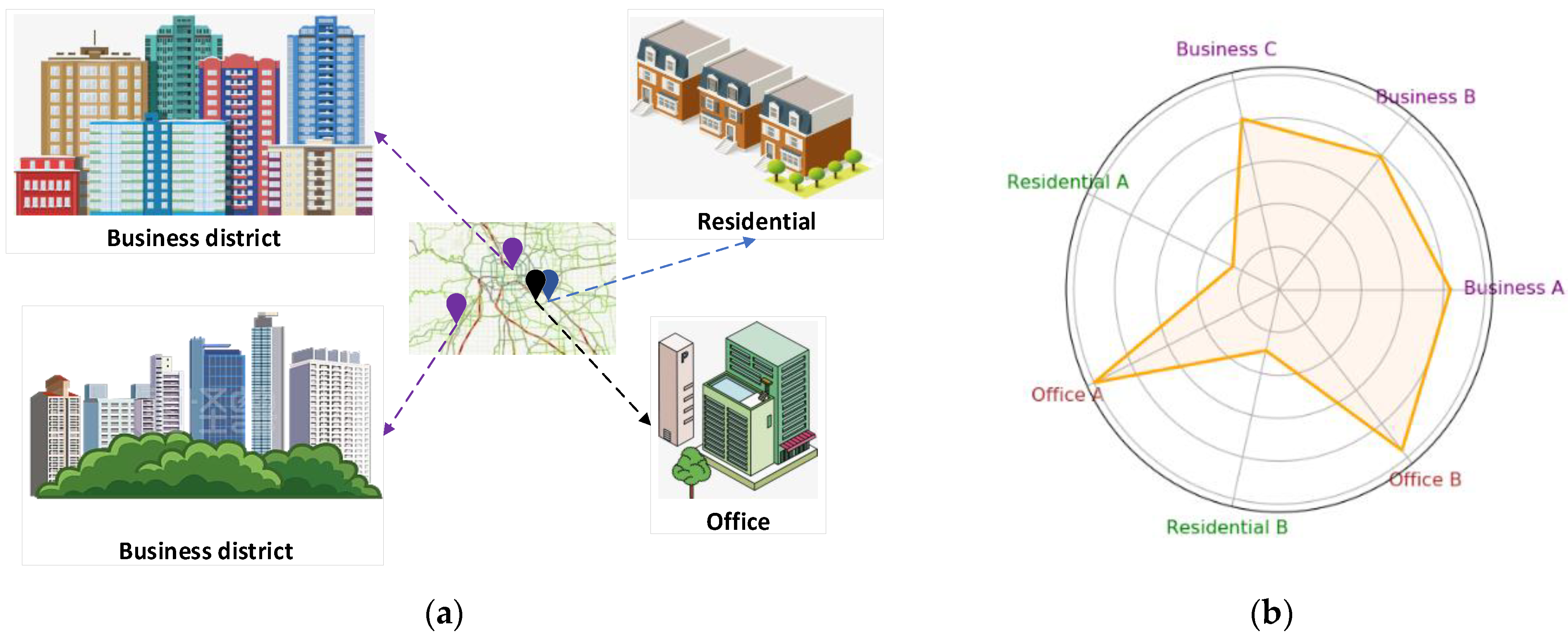
Interregional dependencies: Existing GCN-based spatio-temporal modelling approaches usually build traffic models based on traffic data from the basic road network, where nodes denote road segments or sensor nodes in the basic traffic network graph and edges denote pairs of related road segments or sensor nodes. However, these approaches ignore the inter-regional dependencies in the road network. As shown in Figure 1a, although two geographically distant business districts are spatially separated, they both have similar urban functions as they are dominated by commercial activities, which makes their traffic flow patterns show a high degree of similarity (Figure 1b). As a result, their traffic patterns may show a strong correlation (Shen et al., 2018 [19]; Wang and Li, 2017 [20]). On the contrary, even two geographically adjacent areas, such as residential and office areas, may have significantly different traffic flow patterns because of their different urban functions (Figure 1b). This phenomenon highlights the importance of urban function in traffic flow patterns, rather than just spatial distance. Therefore, without comprehensive insight into wider traffic transitions, the model may fail to capture local geographical dependencies and cross-regional semantic relationships, leading to suboptimal prediction results.
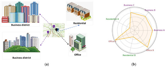
Figure 1.
Illustration of the spatial heterogeneity in traffic flow data. (a) Distribution of geographical areas with different functions. (b) Traffic flows with different urban functions.
Adaptability to dynamic change: An important aspect of the complexity of transport networks is the constant change in road conditions. Most existing models address dynamics by considering both temporal and spatial dimensions. For example, the T-GCN model [21] captures spatial dependencies in complex topologies using GCNs and temporal dependencies in traffic data using GRUs. However, the model relies on predefined adjacency matrices, which limits its application to dynamic traffic network structures. To improve the adaptability of the model, the ASTGCN model [15] introduces an adaptive adjacency matrix. This allows the model to learn the connectivity relationships among nodes from the data dynamically, thus better adapting to different traffic network topologies and spatio-temporal fluctuations; however, its static graph structure may still limit the model’s performance when dealing with more complex spatio-temporal dynamics. Similarly, Graph WaveNet [22] uses an adaptive adjacency matrix, but its reliance on a static adjacency matrix limits its applicability to dynamic traffic networks. AGCRN [23] improves the flexibility and generalisation of the model by dynamically adjusting the adjacency matrix according to the similarity and dynamic changes in historical traffic data. However, the dynamic changes in traffic networks have a certain complexity that cannot be accurately represented by predefined graph structures or adaptive adjacency matrices alone. Therefore, identifying how to capture the dynamic changes in data in a targeted way remains the focus of research.
To address these challenges, we propose a novel self-supervised dynamic spatio-temporal graph convolutional network for traffic flow prediction, called the SDSC model. The proposed SDSC model uses a hierarchical structure to model the dynamic graphs of geographical regions and traffic road networks. The regional graph is mainly constructed by using the traffic network and aggregating geographically similar or functionally similar road sections or regional nodes into regional graph nodes by a clustering method. This approach effectively overcomes the limitation of ignoring inter-regional dependencies in traditional transport network models by modelling across regions. With this approach, the SDSC model is able to capture the cross-regional dependencies among different regions, which improves the model’s performance in global traffic flow prediction. In addition, the SDSC model combines temporal information with dynamic signals to generate dynamic graphs without prior knowledge. It then extracts the spatio-temporal correlations in the dynamic graph through a recursive dynamic graph convolution module. This dynamic graph modelling approach avoids the limitations of predefined graph structures and can flexibly cope with dynamic changes in the traffic network. Compared with the traditional approach based on static adjacency matrices, the SDSC model is better able to cope with fluctuations in the traffic network, thus improving the robustness of the prediction. Finally, by designing a self-supervised learning module based on dynamic and area graphs, the SDSC model is able to maximise the mutual information between the two views, so that the SDSC model can effectively learn traffic flow characteristics from multiple perspectives, thus improving the generalisation ability and accuracy of the model. This design is not only applicable to urban areas that have similar functions but are geographically dispersed (e.g., similar traffic patterns between commercial and business districts), but it is also applicable to urban traffic environments with complex and heterogeneous traffic patterns.
The primary contributions of this paper are summarised below:
A novel dynamic spatio-temporal self-supervised learning traffic prediction model (SDSC) is proposed. The proposed SDSC model enhances the learning of dynamic spatio-temporal features and global area features through self-supervised learning, which can effectively capture the traffic flow dynamics within road networks and improve model performance.
A hierarchical graph neural network architecture is proposed. The upper layer is a dynamic spatio-temporal graph, which introduces a recursive dynamic graph convolution to extract spatiote-temporal correlation features. The lower layer is a region graph, which is constructed based on the similarity in node functionalities within road networks, and graph convolutional is adopted to extract regional features. Then, comprehensive traffic flow features are captured through self-supervised learning.
Experiments on a pair of real-world traffic datasets show that our proposed SDSC method surpasses 17 baseline models.
2. Related Work
2.1. Traditional Traffic Flow Prediction Methods
Initial traffic flow prediction relied mainly on statistical methods, time series analyses, and machine learning techniques. These approaches used historical data patterns and trends to predict future traffic flow. The traditional traffic flow prediction model starts with the historical average model [1], which is known for its simplicity and efficiency. However, simple linear operations cannot fully capture the complex relationships within spatio-temporal sequences. The ARMA model improves on this by modelling and forecasting time series data, capturing trends and periodicities, and is suitable for stable non-seasonal time series. Subsequently, the ARIMA model [2] extends the modelling capability to non-stationary time series based on the ARMA model, but it remains primarily applicable to static time data, limiting its ability to estimate and predict the state of dynamic systems. To address this issue, the Kalman filter model [24] is proposed, which allows linear estimation and prediction of dynamic systems. However, its performance is relatively weak in dealing with non-linear relationships. The KNN method [4] exploits the information in neighbouring samples for prediction, shows a better fitting ability for nonlinear relationships, and is widely used in classification and regression tasks. Meanwhile, SVR [3] uses the kernel function to project the original space into a higher dimensional feature space, constructing a linear model to capture nonlinear relationships. However, its ability to express complex nonlinear relationships is limited, and it cannot efficiently learn high-level abstract feature representations from the original data.
2.2. Deep Learning-Based Traffic Flow Prediction Methods
Deep learning models are adept at handling complex data and tasks through end-to-end learning, powerful feature learning capabilities, and nonlinear modelling capabilities. They have achieved significant success in various domains such as image recognition [25], speech recognition [26], and natural language processing [27]. Notably, they have also achieved remarkable results in the field of traffic flow prediction. Convolutional neural networks (CNNs) [28,29,30] are effective deep learning models that exploit spatial correlations in the data, significantly reducing the number of trainable parameters. This optimisation improves the efficiency of back-propagation algorithms during network propagation. Recurrent Neural Networks (RNNs) [31,32,33] excel at processing sequential data and are adept at effectively extracting temporal and semantic information. Long Short-Term Memory Networks (LSTMs) [6], a variant of RNNs, can solve the gradient vanishing problem present in RNNs by introducing mechanisms such as forgetting gates, input gates, and output gates, thus avoiding the problem of long-term dependence. The gated recurrent unit (GRU) [34] is a simplified variant of LSTM that retains its efficiency while reducing model complexity.
2.3. Graph Convolutional Networks
Traffic road networks typically have a graph structure, and traditional deep learning networks often struggle to capture complex spatio-temporal features. Graph convolutional networks (GCNs) [10] are a type of convolutional neural network specifically designed to work directly with graph data, exploiting the intrinsic structural information to learn intricate relationships among nodes. As a result, GCNs have emerged as a leading deep learning technique in traffic flow prediction. Their key feature is the ability to structure a graph and extract features from neighbouring nodes through hierarchical convolutional operations. Graph convolutional networks have been widely applied in traffic network prediction, benefiting from their powerful feature extraction and representation capabilities. Yu et al. [35] proposed the STGCN model, which uses Chebyshev almost-graphic convolution to capture spatial dependencies and a gated convolutional neural network (gate-CNN) to model temporal dependencies, improving training speed and reducing parameters. SDGCN [36] uses GCNs to extract spatial features and gated recurrent units (GRUs) to extract temporal features. This model improves the ability to model complex roads to some extent, but it performs better with sparse data than with dense data. The ST-CGCN model [37] consists of graph convolution operators, complex correlation matrices, and residual units, which provides greater flexibility in dealing with spatial correlation. In addition, its temporal feature extraction module combines 3D convolution operators and Long Short-Term Memory (LSTM) to improve temporal correlation accuracy significantly. The model performs well with complex spatio-temporal data and is applicable to different types of spatio-temporal data, including dense and sparse data. ADGCN [38] proposes asynchronous spatio-temporal graph convolution (ASTGC), based on the consideration of asynchronous spatio-temporal correlation of transport networks, and combines ASTGC with extended causal convolutional networks to achieve the effect of higher prediction accuracy with fewer parameters.
The attention mechanism, a key deep learning technique, plays an important role in processing sequences, graphical data, etc. It allows models to dynamically focus on different parts of the input data to better capture key information. GCN models incorporating the attention mechanism have shown excellent results. For example, GMAN [39] uses an encoder–decoder structure, where both the encoder and the decoder consist of multiple spatio-temporal attention blocks. This structure is able to capture the spatio-temporal dependencies in the input data dynamically, thus improving the performance of the model in tasks such as traffic flow prediction. In addition, ASTGAT [40] uses a graph attention network (GAT) based on multiple self-attention to model spatial dependencies among different time periods dynamically. This method can effectively capture the spatio-temporal correlations in traffic data and improve the accuracy of the model in predicting traffic flow. In addition, AMGCRN [16] uses the dot product attention mechanism to construct an adaptive graph to extract the similarity of road structures and uses the graph attention mechanism to improve the extraction of local traffic flow features. This approach can effectively handle complex traffic network structures and improve the performance of the model in traffic data analysis. PE-MFSTC [41] further improves the ability to capture complex spatio-temporal dynamics by embedding the peak time into the multirelational synchronous graph attention network, demonstrating the superiority in handling complex traffic scenarios.
However, although the above models improve the performance of traffic flow prediction to some extent, they still lack the comprehensiveness of feature extraction. For example, CGGCN [42] improves the ability to capture dynamic traffic patterns by learning the adjacency matrix, but it is still limited by a predefined graph structure and lacks flexibility in dealing with complex traffic networks. Similarly, HTSTGC [43] effectively solves the problem of heterogeneity in spatio-temporal features, but it ignores potential cross-region dependencies and fails to capture the comprehensive global dynamics of traffic networks. In addition, TPSSL [44] improves the robustness of the model through adaptive data masking, but it still faces challenges in comprehensively dealing with the global features of dynamic spatio-temporal graphs. In addition, STGNN-ANS [45] generates a more flexible graph structure by introducing a neighbour selection mechanism, but a fixed graph structure may limit its performance when dealing with dynamic changes. STFGCN [46], although improved in terms of multi-scale time dependence, still fails to deal adequately with cross-region dynamic changes in traffic networks. In this paper, we not only consider the impact of cross-regional dependence on global prediction accuracy but also comprehensively consider the dynamic characteristics of traffic networks. By comprehensively considering these factors, our proposed model aims to improve performance in the traffic flow prediction task and overcome the limitations of existing models, thus improving the overall prediction accuracy.
3. Preliminaries
Definition 1.
Traffic flow graph. We define the traffic road network as the graph , where denotes the node set of sensors distributed in the traffic road network, and the number of nodes is . denotes the connection relationship among nodes, i.e., the set of edges. is the adjacency matrix of nodes, and denotes the connection relationship between node and node .
Definition 2.
Traffic data. Traffic data represent the observations from all sensors in the traffic flow graph , where is the traffic characteristics captured by the sensors. Our framework involves dividing the data into time steps, and then the input data for each time step is , .
Problem statement. Suppose that the traffic data represent the observations of all sensors in the traffic flow graph , where is the traffic characteristics captured by the sensors. Then, our job is to learn a mapping function that graphs historical data for time steps in the traffic flow data to future traffic data for time steps. The problem is defined by the formula
4. Methods and Materials
The proposed SDSC model addresses the following: (1) capturing the dynamic correlations in spatio-temporal features and (2) capturing comprehensive spatio-temporal features. As illustrated in Figure 2, the model includes the following parts: the graph construction module and the feature learning module.
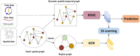
Figure 2.
Overall framework of SDSC.
In the graph construction module, the input data are first used to construct the original adjacency matrix. Dynamic features are then extracted using a multilayer perceptron (MLP) and an attention mechanism. These features are fused with the original adjacency matrix to form a dynamic spatio-temporal graph. Concurrently, a K-means clustering algorithm is employed to classify the data in the original adjacency matrix into different clusters based on node similarity. Each cluster is considered as a feature set, representing specific regions and forming a region graph.
In the feature learning module, dynamic features are learned using a recurrent-based dynamic graph convolutional network (RDGC), while regional features are captured using a graph convolutional network. Finally, self-supervised learning maximises the mutual information of the features learned through the two graph networks, capturing comprehensive traffic flow features and enabling traffic flow prediction.
4.1. Graph Construction Module
4.1.1. Construction of the Spatio-Temporal Dynamic Graph
The spatio-temporal dynamic graph aims to capture the dynamic changes in traffic data and the graph structure. By accounting for changes in both, the model can better understand the evolution of the graph structure and changes in the traffic data, thus improving the accuracy and flexibility of the predictions.
The construction of the spatio-temporal dynamic graph is mainly used to generate initial temporal traffic signal graphs by introducing temporal information, traffic flow, and spatial data. The traffic flow data and the traffic graph are divided into time steps and input into a recursive dynamic graph convolutional network (RDGC) consisting of dynamic graph convolutional gating mechanism (DGCRU) modules for feature extraction to obtain the dynamic graph features . In each time step, the DGCRU module integrates the graph convolution and gating mechanism to capture the changes in graph structure and dynamic traffic to update the input historical data in the current time step and generate the dynamic graph features for the current time step , i.e.,
where is the traffic graph of the current time step containing spatial structure information and is the dynamical graph features of the previous time step. The obtained new dynamic graph features are passed to the multilayer perceptron (MLP) layer for feature extraction, which maps the learned dynamic features into a feature matrix :
The feature matrix is passed to the attention module to compute the attention weights of each node to obtain the weight matrix :
where the weight matrix reflects the importance of each node in the graph. Based on this weight matrix, combined with the traffic graph input in that time step, a cross-feature approach is used to construct a dynamic spatio-temporal graph :
This method is able to model the spatio-temporal dynamic features more accurately by combining the attention weights of the nodes and the spatial graph structure, thus improving the accuracy and robustness.
4.1.2. Regional Graphs
In this paper, the K-means clustering algorithm is applied to identify similar features in the original graph structure and divide it into multiple clusters. This approach ensures a more balanced spread of samples across the dataset, reducing the effect of imbalanced data. Additionally, the clustering operation can extract stable patterns and rules within each cluster, which helps to better handle noise and variations in the data. Ultimately, the accuracy and robustness of the graph structure are significantly improved after clustering analysis.
Specifically, the input data are first used to initialise the cluster centres by selecting data points as the initial cluster centres, , where represents the position of the -th cluster centre in the -th iteration. Then, for the remaining data points, the distance to each cluster centre is calculated, and the nearest cluster centre is allocated to an individual data point:
where represents the -th data point, represents the cluster to which the -th data point belongs, and denotes the Euclidean distance squared. For each cluster, the mean of all data points in that cluster is computed, and this mean is used as the new cluster centre:
where is an indicator function that outputs 1 if the condition is true and 0 if it is not, and is all of the data points. Formulas (7) and (8) are repeated until the cluster centres no longer change or until a predetermined iteration number is reached. After obtaining the cluster labels of each node, the sum of the weights of each node within the same cluster is calculated based on these cluster labels. For each region , the normalised value of the sum of weights of node to other nodes is calculated as:
where is the normalised value of the sum of the weights between node and other nodes in region , and is the weight from node to node . Then, the adjacency matrix of the region graph is constructed as follows:
where is the set of nodes in the region . Finally, the adjacency matrix of the region graph is obtained by applying the softmax function to :
A detailed overview of graph-structured cluster analysis is reflected in Algorithm 1.
| Algorithm 1. Graph structure cluster analysis. |
| Input: Adjacency matrix (), num_clusters () 1: Applied clustering: KMeans.fit () 2: Gets cluster assignment: cluster_labels = KMeans.predict () 3: Data initialization: new_adj_matrix, cluster_count 4: for i = 1; i < .shape[0]; i++ do 5: for j = 1; j < .shape[1]; j++ do 6: Perform cluster analysis according to Equations (9)–(14). 7: end for 8: end for 9: cluster_i = cluster_labels[i] 10: cluster_j = cluster_labels[j] 11: if cluster_i == cluster_j: 12: new_adj_matrix[cluster_i, cluster_j] += adj_matrix[i, j] 13: cluster_count[cluster_i] += 1 14: end if Output: New adjacency matrix (). |
4.2. Feature Learning Module
The feature learning module includes learning dynamic spatio-temporal features and regional features. Ultimately, employing self-supervised learning to maximise the mutual information between these two types features provides new insights, which contribute to achieving accurate prediction results.
4.2.1. Dynamic Spatio-Temporal Feature Learning
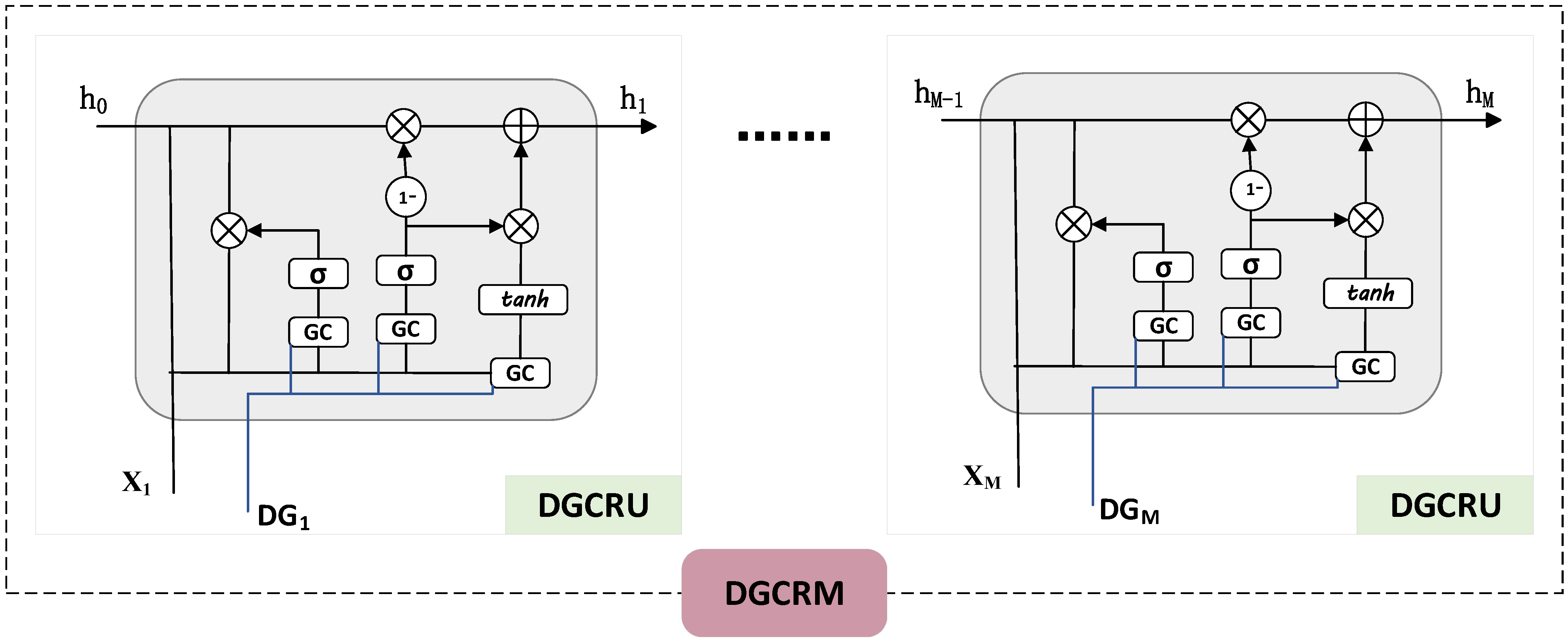
In this paper, we use Recurrent Basic Dynamic Graph Convolution (RDGC) to learn and process features in dynamic spatio-temporal graphs. RDGC consists of multiple dynamic graph convolutional gating mechanism (DGCRU) modules, and the main function of each module is to process the feature information in the spatio-temporal dynamic graphs and generate the dynamic graph features for the next time step through the dynamically adjusted gating mechanism.
As shown in Figure 3, the RDGC framework consists of DGCRU modules stacked on top of each other. Each DGCRU module is used to process complex features in the spatio-temporal dynamic graph and to compute the update gate and reset gate values, which help to capture and update the historical information of the input data .
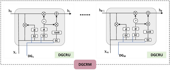
Figure 3.
Framework diagram of RDGC.
In detail, dynamic graph convolution receives and processes dynamic spatio-temporal graph by constructing a normalised Laplace matrix. Specifically, it uses the Laplacian matrix to dot-multiply the dynamic spatio-temporal graph and applies the ReLU activation function to complete the convolution operation:
where is a diagonal matrix at time step , with diagonal elements representing the degrees of each node. By constructing a normalised Laplacian matrix, the dynamic spatio-temporal graph convolution is performed to generate output features :
where is the identity matrix, represents the input features for dynamic graph convolution, and and denote the weight and bias, respectively. In this paper, we update the weight and bias matrices to ensure that their terms vary with the input data in each time step. This adaptation allows both the weight tensor and bias terms to change alongside updates to the traffic signal graph containing temporal information:
In conclusion, the gating value of the spatio-temporal dynamic graph convolution gating mechanism, i.e., the output of the spatio-temporal dynamic graph convolution is as follows:
Accordingly, the spatio-temporal dynamical graph convolutional gating mechanism can be represented as:
where σ denotes the sigmoid activation, , , , , , and denote learnable parameters, denotes the concatenation operation, represents intermediate temporary variables, and, finally, is the output value of the graph convolutional gating mechanism in the -th time step, which is also the dynamic feature in the -th time step. Therefore, the dynamic feature is the sum of the dynamic features over time steps:
The DGCRU module not only extracts features through dynamic graph convolution, but it also incorporates a gating mechanism to learn the dynamics of the features, thus generating dynamic features with time dependence. This approach significantly improves the performance of spatio-temporal graph models when dealing with dynamic data.
4.2.2. Regional Feature Learning
In region graph feature learning, we use a graph convolution network based on Chebyshev polynomials to process the features of region graphs. First, we construct the Chebyshev polynomial support set for performing convolution operations on region graphs . Specifically, we generate Chebyshev polynomials using the following recurrence relation:
where and are initial polynomials, usually taken as and , i.e., the unit matrix and the adjacency matrix of the region graph . With this recurrence relation, we can generate a series of polynomials to perform convolution operations on the region graph to extract the features of the region graph. Next, we use these Chebyshev polynomials to perform a convolution operation on the input features of the region graph to obtain the feature representation of the region graph:
where is the maximum order of the polynomial. Then, we linearly transform the convolution result by including the weights and the bias term to obtain the final output features :
Through this method, we are able to integrate the structural information of the area graph effectively into the feature learning process, so as to extract the important local information in the area graph and improve the expressiveness of the area graph features.
4.2.3. Self-Supervised Learning
We use the InfoNCE loss to optimise the similarity between dynamic graph features and area graph features. First, the original feature vectors are transformed into augmented feature vectors by the feature transformation function . The transformed features are for dynamic graph features and for area graph features . These augmented feature vectors are used in the comparative learning process.
For positive sample pairs, we compute the similarity between the original feature and its extended version. Specifically, the cosine similarity between and is computed, denoted as , and the cosine similarity between and is denoted as . The cosine similarity formula is:
For negative sample pairs, we compute the similarity between the augmented features and the negative samples. Let be the negative sample feature vector and compute and :
The InfoNCE loss function is used to maximise the similarity between pairs of positive samples while minimising the similarity between positive and negative samples. Specifically, the loss function is:
where is the similarity between pairs of positive samples and is the similarity between positive and negative samples, is a temperature parameter to control the smoothness of the contrast, and Q is the number of negative samples.
After completing comparative learning, we splice the dynamic features and the area graph features and further transform them through the fully connected layer to output the final prediction results . The specific operation is:
where and are the weights and bias terms for feature fusion, and and denote the weights and bias terms of the output layer, respectively. With this approach, we are able to align pairs of positive samples in feature space, effectively increasing the discriminative power of the features and thus improving the performance of the model in downstream tasks.
4.3. Loss Function
The loss function is a critical part of the training process for model performance evaluation. By minimising this function, the model effectively diminishes the gap between predicted values and actual labels, thereby enhancing prediction accuracy. We employ L1 loss as the comprehensive training criterion for the entire model. Here, represents historical time steps, denotes future time steps, and signifies the absolute difference between true and predicted values :
Finally, we combine the loss value from the contrastive learning, , with the loss value used to train the entire model, , to obtain the overall loss:
where is a weight parameter for the equalisation of the contributions of the two parts of the loss.
5. Results
5.1. Datasets
To evaluate the performance of the SDSC proposed in this paper, we use two publicly available real traffic flow datasets, PeMSD4 and PeMSD8 [15,47]. These two datasets are from the Caltrans Performance Measurement System (PeMS) [48]. The data were collected in real time from more than 40,000 detectors and were z-score-normalised.
- PeMSD4: This dataset contains traffic flow data from 307 detectors, collected at a frequency of every 5 min for a total data duration of 59 days. The data were collected between January and February 2018;
- PeMSD8: This dataset was provided by 170 detectors, collected at the same frequency of every 5 min, with a total data duration of 62 days, covering the period from July to August 2016.
Specific dataset information is provided in Table 1. These two datasets are from different time periods and geographical regions, covering a wide range of traffic conditions and road types. The PeMSD4 dataset reflects traffic patterns during the winter months of early 2018, while the PeMSD8 dataset provides data from the summer months of 2016. This temporal and seasonal diversity ensures that the data are representative and that the model can be generalised across different traffic conditions. In addition, both datasets provide data with high temporal resolution (collected every 5 min) and include several key metrics (e.g., traffic volumes, average speeds, and occupancy rates), making the data highly representative in both space and time.

Table 1.
Description and statistics of the datasets.
5.2. Experimental Settings
Our experiments were conducted on Windows 10 with an NVIDIA GeForce RTX 2070 GPU. The Python programming language was used during the experiments and the deep learning framework PyTorch was used, specifically, versions Python 3.6.5, PyTorch 1.9.0 and NumPy 1.16.3. To ensure the reproducibility of the experimental results, we set a random seed. The dataset was divided into training, validation, and test sets of 60%, 20%, and 20%, respectively. The training set was used to train the model, the validation set was used to select the best model, and the test set was used to evaluate the final performance of the model. For the hyperparameter settings of the SDSC model, we determined the optimal configuration through several experiments and result comparisons to ensure the efficiency and accuracy of the model. Specifically, we set the hidden layer size of DCGRU to 64, the number of blocks to 2, and the Chebyshev polynomial expansion of order to 2. The embedding dimension was set to 10 for the PEMSD4 dataset and 5 for the PEMSD8 dataset. To ensure effective training and accuracy, the model was trained for 100 epochs and optimised using the Adam optimiser. Because of the high memory requirements of the graph convolution operation and comparison learning, we set specific settings for different datasets as follows: for the PEMSD4 dataset, the batch size was set to 10 and the learning rate was set to 0.0015. While for the PEMSD8 dataset, the batch size was set to 32 and the learning rate was set to 0.003. During the training process, we use the mean absolute error (MAE) as the loss function to measure the accuracy of the model. These settings aim to balance computational resources and model performance to ensure the best results on different datasets.
To evaluate performance, we used the following three metrics: (1) mean absolute error (MAE), (2) root mean square error (RMSE), and (3) mean absolute percentage error (MAPE).
- (1)
- Mean absolute error:
- (2)
- Root mean square error:
- (3)
- Mean absolute percentage error:
5.3. Result Comparison
We evaluated the proposed SDSC against several prominent traffic forecasting methods as follows:
The historical average model (HA) [1] predicts based on the average value of historical observations.
ARIMA [2] combines autoregression (AR), integration (I), and moving average (MA) techniques to model and predict time series data.
VAR [49] is a multivariate linear model used for time series analysis and forecasting.
T-GCN [21] integrates graph convolutional networks (GCNs) with time series models to capture spatio-temporal relationships and dynamic changes in time series data.
STGCN [35] utilises GCN and convolutional neural networks (CNNs) to capture spatial and temporal dependencies in spatio-temporal data.
ASTGCN [15] combines GCN and attention mechanisms to capture spatio-temporal dependencies and adaptively learn important spatio-temporal features.
STSGCN [47] synchronously processes spatial and temporal dimensions to capture correlations and evolutions in spatio-temporal data.
ST-CGCN [37] integrates GCNs and Long Short-Term Memory (LSTM) to represent dynamic spatio-temporal features of complex correlation matrices.
Graph WaveNet [22] combines graph neural networks and WaveNet models to extract hidden spatial features using adaptive matrices.
STFGNN [50] introduces a fusion mechanism to integrate spatial and temporal information effectively.
AGCRN [23] enhances prediction performance by combining attention mechanisms, GCN, and Recurrent Neural Networks (RNN) to learn important relationships among nodes in the traffic network adaptively.
STGODE [51] integrates GNNs and Ordinary Differential Equations (ODEs) to capture dynamic evolution processes in spatio-temporal data.
Z-GCNET [52] presents the notion of temporal zigzag persistence to learn temporal graph structures and improve performance.
STG-NCDE [53] utilises two differential neurocontrol equations to handle the temporal and spatial dimensions of traffic prediction separately.
TBC-GNODE [54] combines Temporal Branch Convolution (TBC) and Graph Neural ODEs, applying refined graph neural differential equations to model the dynamic changes in traffic flow.
STHSGCN [55] designs separate extended causal spatio-temporal synchronous graph convolutional networks and deploys different modules to reflect spatial and temporal heterogeneity, proposing a Causal Spatio-Temporal Synchronous Graph (CSTSG) to capture temporal causality in spatio-temporal synchronous learning.
STFGCN [46] introduces node-specific graph convolution operations to learn specific node patterns and employs an adaptive adjacency matrix to represent the interdependencies among traffic sequences. It also includes a continuous temporal correlation learning module and a Transformer-based global temporal correlation learning module to capture both continuous and global temporal correlations in traffic sequences.
5.4. Experimental Results
Table 2 compares the results of our model against 17 other benchmark models, all evaluated on the PeMSD4 and PeMSD8 datasets. The table highlights that our model achieves optimal performance within 12 time steps. In this paper, the baseline algorithms are divided into traditional methods and GCN-based approaches.

Table 2.
Comparison of SDSC with baseline.
Compared with traditional methods, the SDSC model proposed in this paper significantly outperforms traditional models such as HA, ARIMA, and VAR. Although these traditional methods are capable of handling time series data, they have significant shortcomings in modelling non-linear relationships and focus only on the time dimension, completely ignoring the spatial correlations in traffic flow data. As a result, they are poor at dealing with complex traffic networks and have difficulty capturing potential correlations among different regions. The SDSC model, on the other hand, successfully overcomes these shortcomings by introducing an adaptive neighbourhood structure and a dynamic graph convolution module, and it is able to capture complex traffic flow characteristics in a more comprehensive way.
Compared with the fixed neighbourhood approach, the SDSC model is more adaptable to the dynamic changes in the traffic network. Although STGCN captures spatial information through graph convolutional networks, it has difficultly in adapting to the ever-changing dynamic relationships in the traffic network because of its use of a fixed spatial neighbourhood structure. T-GCN mainly relies on a static graph structure to model spatio-temporal relationships, but its expressiveness is limited when faced with a complex traffic network, and it is unable to exploit the potential network dependencies fully. As a result, these models have shortcomings when dealing with complex and changing traffic flows. Although ASTGCN and STSGCN improve model adaptability by introducing dynamic mechanisms, and ST-CGCN further improves model accuracy by integrating external factors, these improvements are still not comparable to the SDSC model. SDSC significantly improves the model’s ability to cope with dynamic changes in the traffic network by introducing a dynamic neighbourhood structure and a recursive dynamic graph convolution (RDGC) module, which overcomes the limitations of these methods in modelling long and short-term dependencies.
Compared with methods using adaptive structures, the SDSC model also shows greater advantages in dealing with regional dependencies. Although models such as Graph WaveNet, STFGNN, and AGCRN improved their ability to capture traffic flow characteristics by introducing adaptive matrices, their adaptive capabilities are still limited when faced with multi-region and complex network structures. In contrast, SDSC better understands and exploits the complex traffic flow relationships among different regions through cluster analysis. Meanwhile, the self-supervised learning mechanism of SDSC can maximise the mutual information between dynamic and regional graphs, thus significantly improving the prediction accuracy and model robustness.
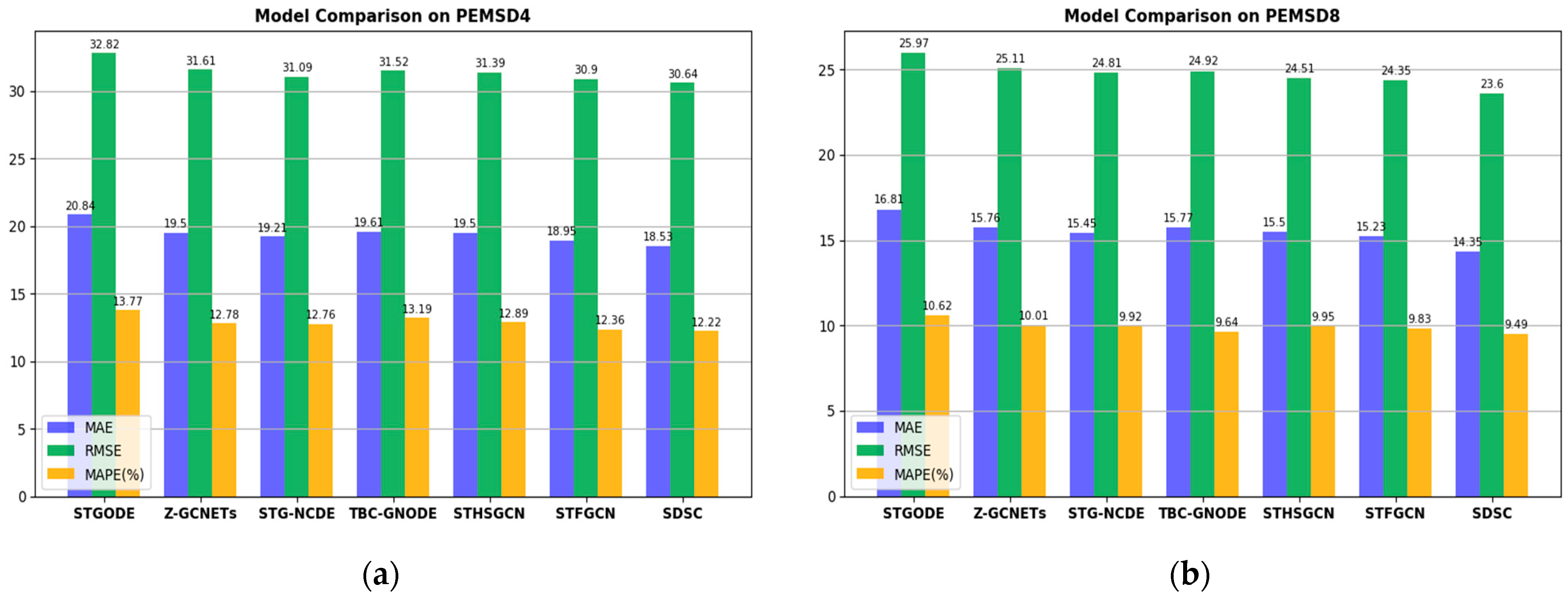
Figure 4 shows the results of our model (SDSC) compared to other recent GCN-based models (e.g., STGODE) on the PEMSD4 and PEMSD8 datasets. SDSC shows significant superiority in the MAE, RMSE, and MAPE metrics on both the PEMSD4 (Figure 4a) and PEMSD8 (Figure 4b) datasets. These results further confirm the superior performance of our model on both datasets.
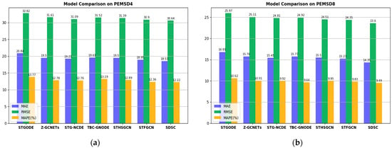
Figure 4.
Comparison of SDSC with other models. (a) Comparison of other recent GCN-based models with SDSC on the PEMSD4 dataset. (b) Comparison of other recent GCN-based models with SDSC on the PEMSD8 dataset.
Therefore, the main reasons why the model in this paper outperforms other models can be attributed to the following: First, by dealing with regional relationships through cluster analysis, the complex traffic flow characteristics among different regions are better understood and exploited, which compensates for the shortcomings of traditional methods when there is insufficient information about traffic transformation at the global level and avoids suboptimal prediction. Secondly, by adopting the adaptive structure method, the model is able to adjust the neighbourhood matrix flexibly, which strengthens the ability to adapt to different traffic network structures and avoids the limitations of fixed neighbourhood structures. Finally, by introducing the dynamic graph convolution recursion module (RDGC) and comparative learning methods (e.g., InfoNCE loss), the model is able to cope with the variability in the complex traffic network effectively and maximise the mutual information between the dynamic graph features and the area graph features, which further improves the prediction performance and robustness of the model.
Overall, the improved performance of the SDSC model can effectively alleviate the urban traffic congestion problem. By more accurately predicting traffic flow, SDSC helps to optimise traffic management and reduce delays and congestion in urban road networks, providing strong support for traffic management in smart cities.
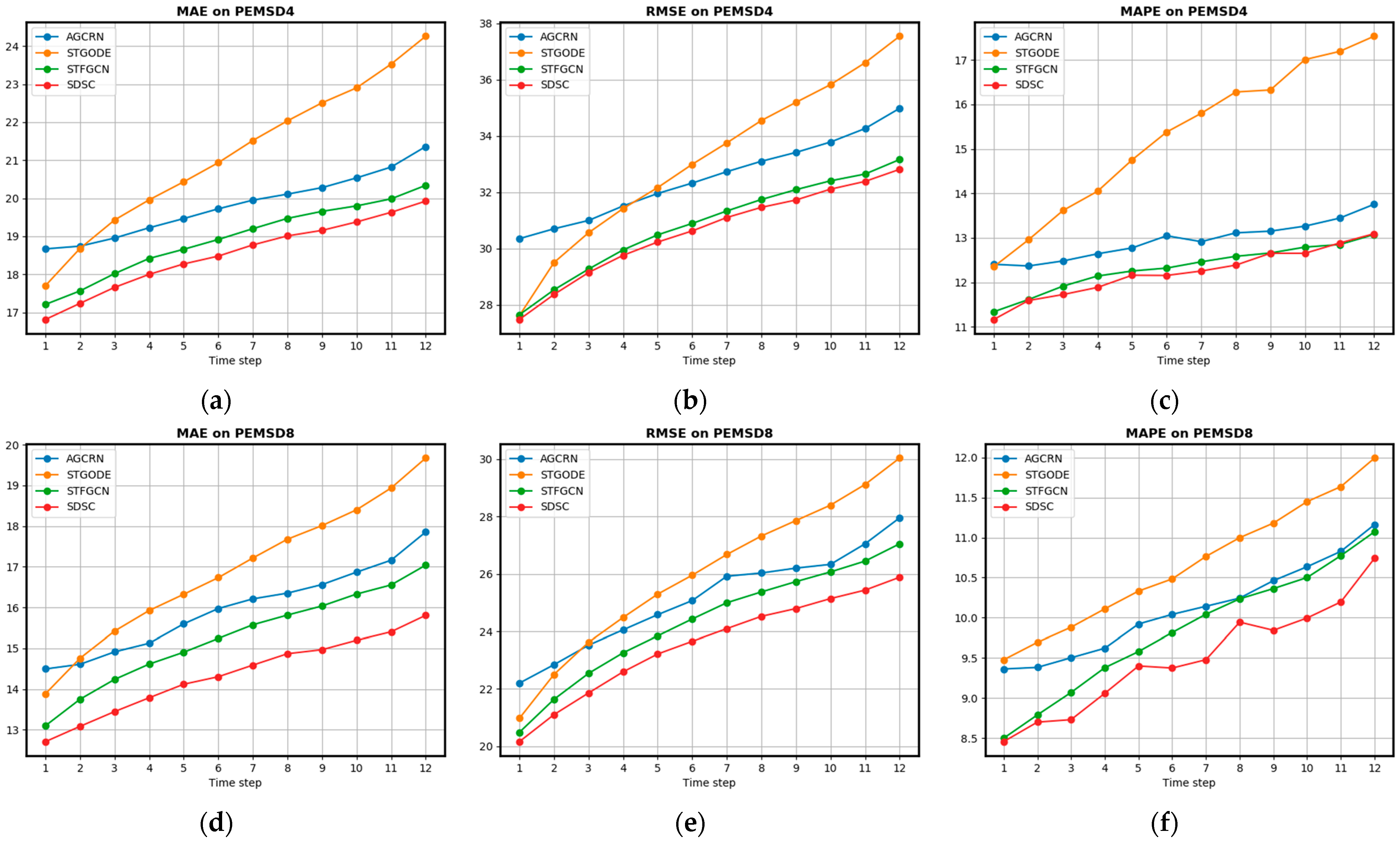
Figure 5 shows the performance comparison between the SDSC model and the representative model in different time steps, where (a), (b), and (c) show a comparison of the MAE, RMSE, and MAPE metrics of each model on the PEMSD4 dataset, and (d), (e), and (f) show the corresponding metrics on the PEMSD8 dataset, respectively. From (a), (b), (d), and (e) in Figure 5, it is clear that the STGODE model outperforms the AGCRN model in the short-term prediction, which is mainly due to its ability to better capture the instantaneous changes in traffic flow in the short-term. However, in the long-term predictions, STGODE has the largest increase in the damage rate and performs relatively poorly, which may be related to its inadequate modelling of long-term dependence. On the other hand, STFGCN outperforms AGCRN in both short- and long-term predictions on both the PEMSD4 and PEMSD8 datasets and is the best performer among these three models. This suggests that STFGCN is more consistent and accurate in dealing with all stages of traffic flow prediction.
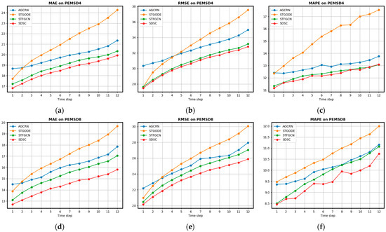
Figure 5.
Comparison of prediction performance in each time step on PEMSD4 and PEMSD8: (a) MAE on dataset PEMSD4; (b) RMSE on dataset PEMSD4; (c) MAPE on dataset PEMSD4; (d) MAE on dataset PEMSD8; (e) RMSE on dataset PEMSD8; and (f) MAPE on dataset PEMSD8.
Comparing the performance of SDSC with that of STFGCN, the SDSC model significantly outperforms STFGCN on the PEMSD4 dataset in terms of the MAE (Figure 5a) and RMSE (Figure 5b) metrics. Specifically, SDSC has a lower MAE and lower RMSE than STFGCN in short-term forecasting, demonstrating its superiority in capturing short-term fluctuations in traffic flows. However, for the MAPE metric (Figure 5c), although SDSC is slightly better for short-term forecasts, its gap with STFGCN is smaller for long-term forecasts. This may be related to the challenges SDSC faces in long-term forecasting, e.g., the ability to capture long-term trends needs to be further improved. On the PEMSD8 dataset (Figure 5d–f), the performance of SDSC is also satisfactory. In particular, SDSC outperforms STFGCN on all indicators, further confirming its effectiveness in predicting traffic flow. This indicates that SDSC not only has superior prediction performance on the PEMSD4 dataset but also performs equally well on the PEMSD8 dataset, highlighting its stability and accuracy on different datasets. Overall, the SDSC model outperforms the STFGCN in most cases, especially in the short-term prediction, where its overall performance is superior.
5.5. Ablation Experiments
To test the impact of major modules on SDSC, we performed ablation experiments. The corresponding ablation names are as follows:
w/o cluster: Without cluster analysis. Instead of using clustering to construct the regional graph, a proximity-based method was used to assess the contribution of clustering to cross-regional semantic relationships.
w/o compare: Without using self-supervised learning to capture the mutual information of features learned by the two graph networks, the two dynamic graph features were directly concatenated to observe the contribution of contrastive learning in the model.
w/o RDGC: Without using RDGC to process dynamic graph features, traditional recursive graph convolution was used instead to extract dynamic graph features to observe the contribution of RDGC in dynamic feature extraction.
w/o GCN: Without using Chebyshev polynomial-based graph convolution to extract regional graph features, simple graph convolution was used to see the contribution of this graph convolution to regional graph feature extraction.
w/o Attention: Without using the attention mechanism to adapt the importance of dynamic information during the construction of dynamic graphs, the importance of the attention mechanism in dynamic graph construction was evaluated.
The values of MAE, RMSE and MAPE for each of the variants on the PeMSD4 and PeMSD8 datasets are shown in Table 3. The specific results are as follows:

Table 3.
Experimental results of variants of SDSC on both databases.
- (1)
- w/o cluster: The ablation results show that this variant exhibits a significant degradation in performance on the PeMSD4 and PeMSD8 datasets. Specifically, the MAE increased from 18.53 to 18.64 on the PEMSD4 dataset and from 14.35 to 14.50 on the PEMSD8 dataset, suggesting that the use of proximity-based rather than clustering to construct the area graph fails to capture cross-area semantic relationships effectively, leading to an increase in prediction error. The lack of clustering analysis affects the model’s ability to capture cross-regional traffic flows, making the construction of the area graph less accurate.
- (2)
- w/o compare: The ablation results show a decrease in model performance after omitting the self-supervised learning module. For example, the MAE on the PEMSD4 dataset increases from 18.53 to 18.57 and the RMSE increases from 30.64 to 31.05, highlighting the importance of comparative learning in capturing and integrating dynamic graph features. Without this mechanism, the model is unable to exploit the mutual information between the two graph networks effectively, resulting in lower prediction accuracy.
- (3)
- w/o RDGC: The results show a significant decrease in model performance after removing the recursive dynamic graph convolution module. Specifically, on the PEMSD4 dataset, the MAE improves to 24.82 and the RMSE reaches 38.97. This result suggests that the RDGC module is crucial for capturing spatio-temporal variations in the features of the dynamic graphs, and its absence significantly affects the model’s ability to understand and process the dynamic relationships.
- (4)
- w/o GCN: The use of simple graph convolution instead of Chebyshev polynomial-based graph convolution resulted in a decrease in performance. On the PEMSD4 dataset, the MAE is 18.62 and the RMSE is 31.07, indicating that Chebyshev polynomial-based graph convolution has a significant advantage in extracting features from the region graph and captures the complex relationships among regions more accurately.
- (5)
- w/o Attention: Models that did not use the attention mechanism performed poorly. On the PEMSD4 dataset, the MAE was 18.59 and the RMSE was 30.90, highlighting the importance of the attention mechanism in the construction of the dynamic graphs, which effectively adjusts the importance of the dynamic information to increase the predictive power of the model.
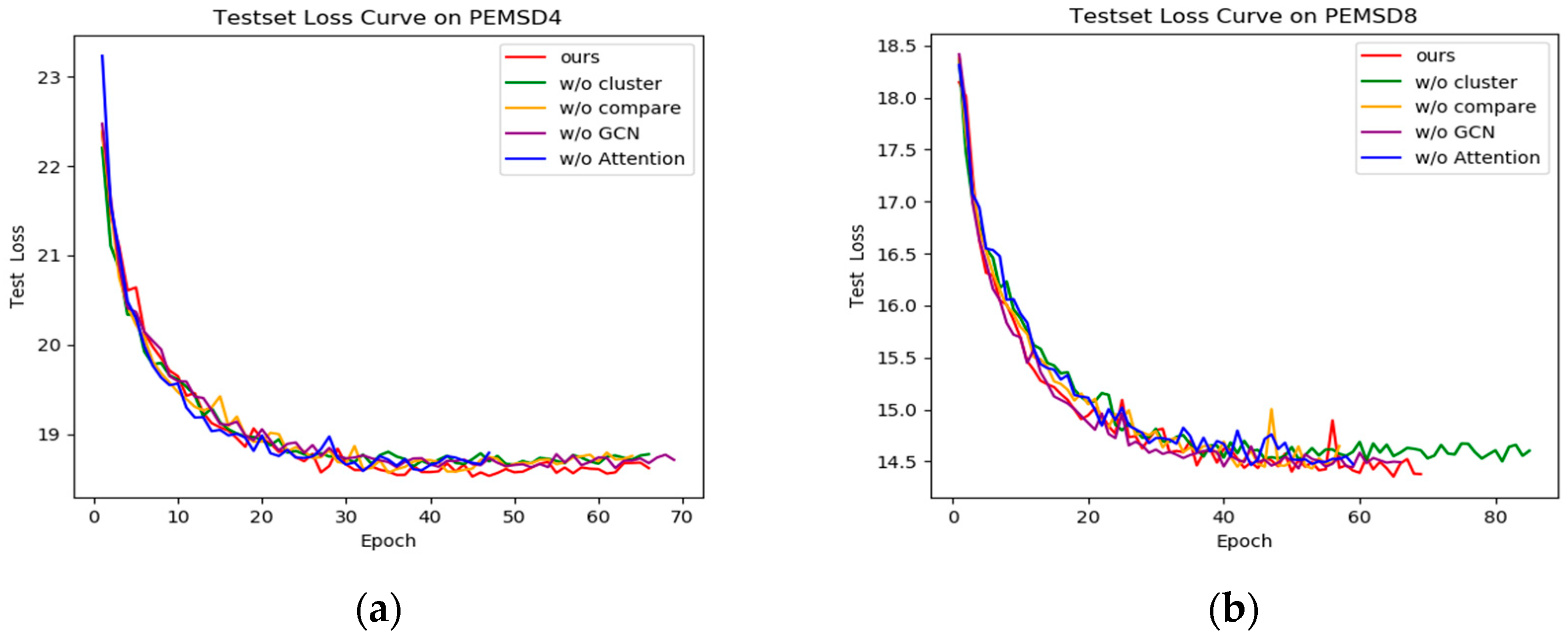
The performance of the variants is further visualised in Figure 6. Since the performance of the w/o RDGC variant is significantly degraded, Figure 6 illustrates the tested loss curves of the other variants on the PEMSD4 and PEMSD8 datasets. Specifically, on the PEMSD4 dataset (Figure 6a), the loss values of w/o cluster, w/o compare, and w/o Attention decrease faster in the early stages, but they are significantly higher than SDSC in the later stages, suggesting that these variants are able to provide some predictive power in the early stages but are unable to maintain the stability of the model performance. In particular, w/o cluster and w/o Attention underperform in handling cross-region data and adjusting dynamic information, resulting in poor model performance in long-term prediction. The w/o GCN variant, on the other hand, has consistently higher loss values than SDSC, further demonstrating the important role of Chebyshev polynomial graph convolution in feature extraction. On the PEMSD8 dataset (Figure 6b), the loss value of the w/o GCN variant decreases fastest in the early stages, but it is slightly higher than SDSC in the later stages, suggesting that simple graph convolution performs better in capturing the early features but has a smoother effect in long-term prediction, failing to take full advantage of the complex regional relationships. In contrast, graph convolution based on Chebyshev polynomials can handle complex features more efficiently in long-term prediction, thus improving the overall performance of the model. In addition, the w/o compare variant has a high loss value in the early rounds, and although it is close to SDSC in the final rounds, its overall performance is still poor, suggesting that comparative learning plays a key role in improving the performance and stability of the model. The loss values of w/o cluster and w/o Attention, on the other hand, are higher than those of SDSC in every stage, highlighting the indispensability of cluster analysis and attention mechanisms for model performance. In summary, the key modules have varying degrees of influence on the performance of the SDSC model. Each module plays an important role in the accuracy and robustness of the model, and its absence significantly reduces the overall performance of the model.
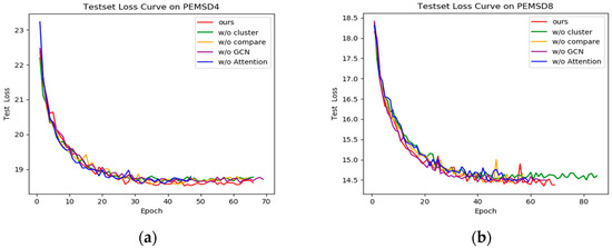
Figure 6.
Test set loss curves for various variants. (a) Test set loss curves on PEMSD4. (b) Test set loss curves on PEMSD8.
6. Discussion
6.1. Parametric Analysis
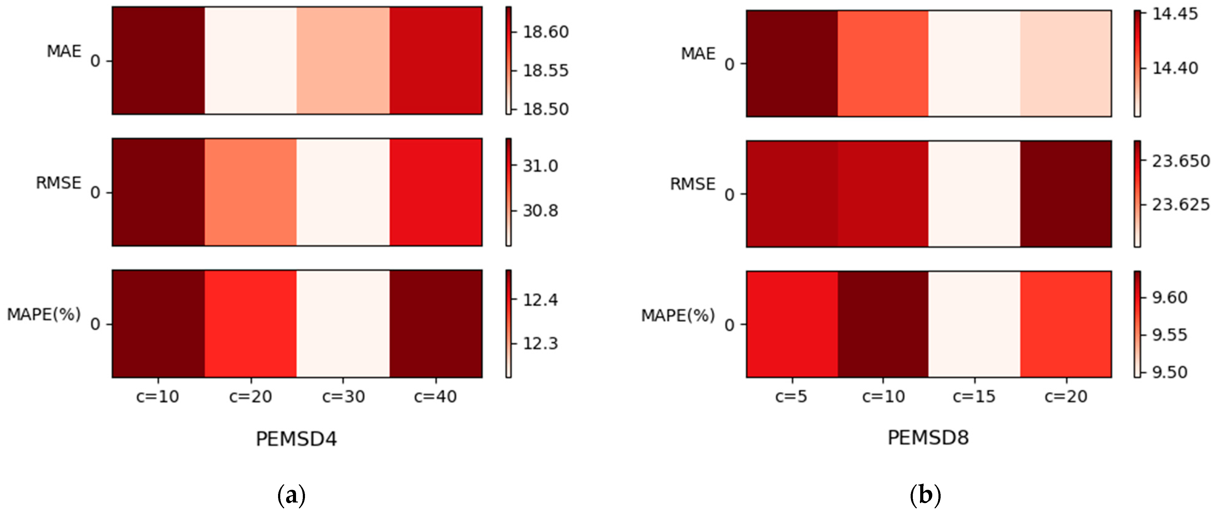
The performance of the model is significantly affected by the parameter settings, especially the choice of core parameters such as the number of clusters . We analysed the effect of different numbers of clusters on the model performance and presented the experimental results through heatmaps (Figure 7). On the PeMSD4 dataset (Figure 7a), the worst results are obtained when the number of clusters is set to = 10 and = 40, an effect that may be due to the fact that these cluster values lead to too extreme aggregation or segmentation of the data, which loses important detailed information or leads to excessive dispersion of information. This is consistent with our model performance assumption that the number of clusters should be chosen to balance the detail and overall structure of the data in order to improve the predictive accuracy of the model. Relatively, the best results were obtained with = 30, indicating that this setting is effective in preserving the details of the data while maintaining the overall structure of the data. While on the PeMSD8 dataset (Figure 7b), the results show the best results with = 15. This result is different from the optimal cluster setting on the PeMSD4 dataset, indicating that the optimal number of clusters varies depending on the characteristics, size, and intrinsic structure of the dataset. These experimental results not only highlight the importance of parameter selection but also point to the need for different parameter settings for different datasets. This finding helps us to better understand the characteristics of the data and provides guidance on how to adjust the model parameters according to the specifics of the dataset in order to maximise the prediction performance.
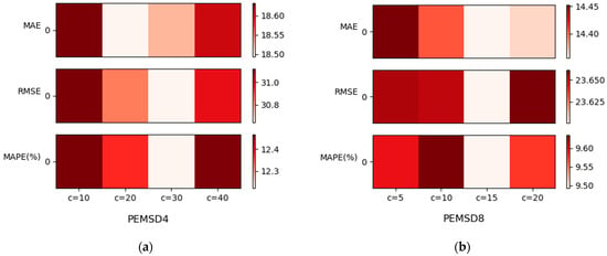
Figure 7.
Effect of the number of clusters on PeMSD4 and PeMSD8. (a) Effect of the number of clusters on PeMSD4. (b) Effect of the number of clusters on PeMSD8.
6.2. Computation Cost
When evaluating the practical application of traffic flow prediction models, it is crucial to match the complexity of the SDSC model with the actual requirements. The computational data in Table 4 show that the complexity of the SDSC model is still within acceptable limits, despite the increase in training and inference time compared with the other benchmark models (e.g., AGCRN, STGODE, and STG-NCDE). For example, on the PEMSD4 dataset, the training time for SDSC is 124.3 s/round and the inference time is 12.8 s; on the PEMSD8 dataset, the training time is 45.4 s/round and the inference time is 4.6 s. In comparison, STG-NCDE has a training time of 118.6 s/round and an inference time of 12.3 s, suggesting that the computational cost of SDSC is slightly higher but comparable to the current state of the art.

Table 4.
The computation time on PEMSD4 and PEMSD8 datasets.
The SDSC model significantly improves the accuracy of traffic flow prediction by introducing dynamic graph convolution and self-supervised learning techniques. This improvement not only optimises the accuracy of traffic flow prediction but also significantly enhances the effectiveness of traffic management and planning. Experimental results show that SDSC outperforms 20 benchmark models on multiple datasets, validating its effectiveness in practical applications.
In addition, with the development of computer hardware and the advancement of technology optimisation, the training and inference time of the SDSC model is expected to be further improved. In terms of prediction accuracy and computational cost, the complexity of the SDSC model fully meets the requirements of real-world applications and shows significant advantages in improving prediction performance.
7. Conclusions
In this paper, a new self-supervision-based dynamic spatio-temporal traffic prediction model (SDSC) is proposed, which overcomes the limitations of traditional methods in capturing complex spatio-temporal dependencies through an innovative spatio-temporal graph neural network architecture and accurately captures and predicts the subtle changes in traffic flow in a dynamic and changing traffic environment. Secondly, the clustering method is used to capture the global dependencies of the original data, which enhances the regional feature representation. Through a self-supervised learning mechanism, the model further extracts and fuses key features from the dynamic and regional graphs to achieve more accurate traffic flow prediction. This approach not only improves the adaptability and robustness of the model but also provides a stronger database for ITS optimisation and decision support. In practical applications, the SDSC model can effectively support the accurate prediction of urban traffic flow to optimise traffic management strategies, reduce congestion, and improve road use efficiency.
Despite the excellent performance of SDSC, the two modules of dynamic graph convolution and self-supervised learning make the SDSC model have high complexity. Through ablation experiments, we can see that removing these modules leads to significant performance degradation, suggesting that they play a key role in the model. However, this may also be challenging in large-scale datasets or real-time applications, and optimisation of the model (e.g., pruning, knowledge distillation) needs to be considered to improve its efficiency in real-world applications. Secondly, improving the model’s ability to capture long-term dependencies is also an important research direction, which will help the model to better handle long-term traffic flow trends. Finally, more external data sources, such as weather and event information, can be introduced to improve the prediction accuracy. These improvements will further enhance the performance and practical application value of the SDSC model.
Author Contributions
Conceptualisation, Y.S. and C.W.; methodology, Y.S.; software, C.W.; validation, S.W., Y.S. and R.G.; formal analysis, Y.S. and S.S.; investigation, D.L.; resources, S.W. and C.W.; data curation, Y.S.; writing—original draft preparation, Y.S.; writing—review and editing, Y.S. and D.L.; visualisation, Y.S. and S.S.; supervision, C.W. and R.G.; project administration, C.W. and D.L.; funding acquisition, C.W., R.G. and D.L. All authors have read and agreed to the published version of the manuscript.
Funding
This work was supported in part by the National Natural Science Foundation of China under Grants 62206116, the Chunhui Plan Collaborative Research Project, Ministry of Education, China (HZKY20220350), and the Key R&D Plan of Hubei Provincial Department of Science and Technology 2023BCB041.
Institutional Review Board Statement
Not applicable.
Informed Consent Statement
Not applicable.
Data Availability Statement
The PMES04 dataset and the PEMS08 dataset were accessed on 1 October 2023 via https://github.com/MengzhangLI/STFGNN.
Acknowledgments
We thank the teachers and students for their help and support, and the editors and anonymous reviewers for their valuable comments and suggestions.
Conflicts of Interest
Author S.W. is employed by the company CCCC Second Highway Consultants Co., Ltd., and the author’s position in the company is Senior Mechanical and Electrical Engineer. The remaining authors declare that this research was conducted in the absence of any commercial or financial relationships that could be construed as a potential conflict of interest.
References
- Jing, L.; Wei, G. A Summary of Traffic Flow Forecasting Methods. J. Highw. Transp. Res. Dev. 2004, 21, 82–85. [Google Scholar]
- Williams, B.M.; Hoel, L.A. Modeling and Forecasting Vehicular Traffic Flow as a Seasonal ARIMA Process: Theoretical Basis and Empirical Results. J. Transp. Eng. 2003, 129, 664–672. [Google Scholar] [CrossRef]
- Drucker, H.; Burges, C.J.; Kaufman, L.; Smola, A.; Vapnik, V. Support vector regression machines. In Proceedings of the Annual Conference on Neural Information Processing Systems, Denver, CO, USA, 2–5 December 1996; Volume 9, pp. 155–161. [Google Scholar]
- Cover, T.M.; Hart, P.E. Nearest neighbor pattern classification. IEEE Trans. Inf. Theory 1953, 13, 21–27. [Google Scholar] [CrossRef]
- Krizhevsky, A.; Sutskever, I.; Hinton, G. ImageNet Classification with Deep Convolutional Neural Networks. In Proceedings of the Annual Conference on Neural Information Processing Systems, Lake Tahoe, NV, USA, 3–6 December 2012; Volume 25. [Google Scholar]
- Hochreiter, S.; Schmidhuber, J. Long Short-term Memory. Neural Comput. 1997, 9, 1735–1780. [Google Scholar] [CrossRef]
- Mnih, V.; Heess, N.; Graves, A.; Kavukcuoglu, K. Recurrent Models of Visual Attention. In Proceedings of the Annual Conference on Neural Information Processing Systems, Montreal, QC, Canada, 8–13 December 2014; Volume 3. [Google Scholar]
- Bai, S.; Kolter, J.Z.; Koltun, V. An Empirical Evaluation of Generic Convolutional and Recurrent Networks for Sequence Modeling. arXiv 2018, arXiv:1803.01271. [Google Scholar]
- Zhao, W.; Gao, Y.; Ji, T.; Wan, X.; Ye, F.; Bai, G. Deep Temporal Convolutional Networks for Short-Term Traffic Flow Forecasting. IEEE Access 2019, 7, 114496–114507. [Google Scholar] [CrossRef]
- Kipf, T.N.; Welling, M. Semi-Supervised Classification with Graph Convolutional Networks. arXiv 2016, arXiv:1609.02907. [Google Scholar]
- Wang, J.; Chen, Q. A traffic prediction model based on multiple factors. J. Supercomput. 2020, 77, 2928–2960. [Google Scholar] [CrossRef]
- Hu, Y.; Peng, T.; Guo, K.; Sun, Y.; Gao, J.; Yin, B. Graph transformer based dynamic multiple graph convolution networks for traffic flow forecasting. IET Intell. Transp. Syst. 2023, 17, 1835–1845. [Google Scholar] [CrossRef]
- Sui, Y. An Efficient Short-Term Traffic Speed Prediction Model Based on Improved TCN and GCN. Sensors 2021, 21, 6735. [Google Scholar] [CrossRef]
- Shi, T.; Yuan, W.; Wang, P.; Zhao, X. Regional Traffic Flow Prediction on multiple Spatial Distributed Toll Gate in a City Cycle, 2021. In Proceedings of the IEEE 16th Conference on Industrial Electronics and Applications (ICIEA), Chengdu, China, 1–4 August 2021; pp. 94–99. [Google Scholar]
- Guo, S.; Lin, Y.; Feng, N.; Song, C.; Wan, H. Attention Based Spatial-Temporal Graph Convolutional Networks for Traffic Flow Forecasting. In Proceedings of the AAAI Conference on Artificial Intelligence, Honolulu, HI, USA, 27 January–1 February 2019. [Google Scholar]
- Liu, L.; Cao, Y.; Dong, Y.; Li, M.E. Attention-Based Multiple Graph Convolutional Recurrent Network for Traffic Forecasting. Sustainability 2023, 15, 4697. [Google Scholar] [CrossRef]
- Zhang, H.; Chen, L.; Cao, J.; Zhang, X.; Kan, S.; Zhao, T. Traffic Flow Forecasting of Graph Convolutional Network Based on Spatio-Temporal Attention Mechanism. Int. J. Automot. Technol. 2023, 24, 1013–1023. [Google Scholar] [CrossRef]
- Zhang, Q.; Chang, W.; Yin, K.T.M. Attention-Based Spatial-Temporal Convolution Gated Recurrent Unit for Traffic Flow Forecasting. Entropy 2023, 25, 938. [Google Scholar] [CrossRef] [PubMed]
- Shen, B.; Liang, X.; Ouyang, Y.; Liu, M.; Zheng, W.; Carley, K.M. StepDeep: A Novel Spatial-temporal Mobility Event Prediction Framework based on Deep Neural Network. In Proceedings of the 24th ACM SIGKDD International Conference on Knowledge Discovery & Data Mining, London, UK, 19–28 August 2018. [Google Scholar]
- Wang, H.; Li, Z. Region Representation Learning via Mobility Flow. In Proceedings of the 2017 ACM on Conference on Information and Knowledge Management, Singapore, 6–10 November 2017. [Google Scholar]
- Zhao, L.; Song, Y.; Zhang, C.; Liu, Y.; Li, H. T-GCN: A Temporal Graph Convolutional Network for Traffic Prediction. IEEE Trans. Intell. Transp. Syst. 2019, 21, 3848–3858. [Google Scholar] [CrossRef]
- Wu, Z.; Pan, S.; Long, G.; Jiang, J.; Zhang, C. Graph WaveNet for Deep Spatial-Temporal Graph Modeling. arXiv 2019, arXiv:1906.00121. [Google Scholar]
- Bai, L.; Yao, L.; Li, C.; Wang, X.; Wang, C. Adaptive Graph Convolutional Recurrent Network for Traffic Forecasting. In Proceedings of the Annual Conference on Neural Information Processing Systems, Online, 6–12 December 2020; Volume 33, pp. 17804–17815. [Google Scholar]
- Kalman, R.E. A New Approach to Linear Filtering and Prediction Problems. J. Fluids Eng. 1959, 82, 35–45. [Google Scholar] [CrossRef]
- Cheng, G.; Yang, C.; Yao, X.; Guo, L.; Han, J. When Deep Learning Meets Metric Learning: Remote Sensing Image Scene Classification via Learning Discriminative CNNs. IEEE Trans. Geosci. Remote Sens. 2018, 56, 2811–2821. [Google Scholar] [CrossRef]
- Saon, G.; Tueske, Z.; Bolanos, D.; Kingsbury, B. Advancing RNN Transducer Technology for Speech Recognition. In Proceedings of the ICASSP 2021-2021 IEEE International Conference on Acoustics, Speech and Signal Processing (ICASSP), Toronto, ON, Canada, 6–11 June 2021. [Google Scholar]
- Gu, Y.; Tinn, R.; Cheng, H.; Lucas, M.; Usuyama, N.; Liu, X.; Naumann, T.; Gao, J.; Poon, H. Domain-Specific Language Model Pretraining for Biomedical Natural Language Processing. ACM Trans. Comput. Healthc. 2020, 3, 1–23. [Google Scholar] [CrossRef]
- Lin, Z.; Feng, J.; Lu, Z.; Li, Y.; Jin, D. DeepSTN+: Context-Aware Spatial-Temporal Neural Network for Crowd Flow Prediction in Metropolis. In Proceedings of the AAAI Conference on Artificial Intelligence, Honolulu, HI, USA, 27 January–1 February 2019; pp. 1020–1027. [Google Scholar]
- Zhang, J.; Zheng, Y.; Qi, D. Deep Spatio-Temporal Residual Networks for Citywide Crowd Flows Prediction. In Proceedings of the AAAI Conference on Artificial Intelligence, San Francisco, CA, USA, 4–9 February 2016. [Google Scholar]
- Yao, H.; Tang, X.; Wei, H.; Zheng, G.; Li, Z. Revisiting Spatial-Temporal Similarity: A Deep Learning Framework for Traffic Prediction. In Proceedings of the AAAI Conference on Artificial Intelligence, Honolulu, HI, USA, 27 January–1 February 2019. [Google Scholar]
- Ye, J.; Sun, L.; Du, B.; Fu, Y.; Xiong, H. Coupled Layer-wise Graph Convolution for Transportation Demand Prediction. In Proceedings of the AAAI Conference on Artificial Intelligence, New York, NY, USA, 7–12 February 2020. [Google Scholar]
- Li, Y.; Yu, R.; Shahabi, C.; Liu, Y. Diffusion Convolutional Recurrent Neural Network: Data-Driven Traffic Forecasting. arXiv 2017, arXiv:1707.01926. [Google Scholar]
- Li, F.; Feng, J.; Yan, H.; Jin, G.; Yang, F.; Sun, F.; Jin, D.; Li, Y. Dynamic Graph Convolutional Recurrent Network for Traffic Prediction: Benchmark and Solution. ACM Trans. Knowl. Discov. Data 2023, 17, 1–21. [Google Scholar] [CrossRef]
- Chung, J.; Gulcehre, C.; Cho, K.H.; Bengio, Y. Empirical Evaluation of Gated Recurrent Neural Networks on Sequence Modeling. arXiv 2014, arXiv:1412.3555. [Google Scholar]
- Yu, B.; Yin, H.; Zhu, Z. Spatio-Temporal Graph Convolutional Networks: A Deep Learning Framework for Traffic Forecasting. arXiv 2017, arXiv:1709.04875. [Google Scholar]
- Liang, G.; U, K.; Ning, X.; Tiwari, P.; Nowaczyk, S.; Kumar, N. Semantics-Aware Dynamic Graph Convolutional Network for Traffic Flow Forecasting. IEEE Trans. Veh. Technol. 2023, 72, 7796–7809. [Google Scholar] [CrossRef]
- Bao, Y.; Huang, J.; Shen, Q.; Cao, Y.; Ding, W.; Shi, Z.; Shi, Q. Spatial–Temporal Complex Graph Convolution Network for Traffic Flow Prediction. Eng. Appl. Artif. Intel. 2023, 121, 106044. [Google Scholar] [CrossRef]
- Qi, T.; Li, G.; Chen, L.; Xue, Y. ADGCN: An Asynchronous Dilation Graph Convolutional Network for Traffic Flow Prediction. IEEE Internet Things J. 2021, 9, 4001–4014. [Google Scholar] [CrossRef]
- Zheng, C.; Fan, X.; Wang, C.; Qi, J. GMAN: A Graph Multi-Attention Network for Traffic Prediction. In Proceedings of the AAAI Conference on Artificial Intelligence, New York, NY, USA, 7–12 February 2020; Volume 34, pp. 1234–1241. [Google Scholar]
- Wang, Y.; Jing, C.; Xu, S.; Guo, T. Attention based spatiotemporal graph attention networks for traffic flow forecasting. Inf. Sci. 2022, 607, 869–883. [Google Scholar] [CrossRef]
- Wei, S.; Hu, D.; Wei, F.; Liu, D.; Wang, C. Traffic flow prediction with multi-feature spatio-temporal coupling based on peak time embedding. J. Supercomput. 2024, 80, 23442–23470. [Google Scholar] [CrossRef]
- Xu, J.; Huang, X.; Song, G.; Gong, Z. A coupled generative graph convolution network by capturing dynamic relationship of regional flow for traffic prediction. Clust. Comput. 2024, 27, 6773–6786. [Google Scholar] [CrossRef]
- Xu, J.; Li, Y.; Lu, W.; Wu, S.; Li, Y. A heterogeneous traffic spatio-temporal graph convolution model for traffic prediction. Phys. A Stat. Mech. Its Appl. 2024, 641, 129746. [Google Scholar] [CrossRef]
- Gao, M.; Wei, Y.; Xie, Y.; Zhang, Y. Traffic Prediction with Self-Supervised Learning: A Heterogeneity-Aware Model for Urban Traffic Flow Prediction Based on Self-Supervised Learning. Mathematics 2024, 12, 1290. [Google Scholar] [CrossRef]
- Sun, H.; Tang, X.; Lu, J.; Liu, F. Spatio-Temporal Graph Neural Network for Traffic Prediction Based on Adaptive Neighborhood Selection. Transp. Res. Rec. 2024, 2678, 641–655. [Google Scholar] [CrossRef]
- Ma, Y.; Lou, H.; Yan, M.; Sun, F.; Li, G. Spatio-temporal fusion graph convolutional network for traffic flow forecasting. Inf. Fusion 2024, 104, 102196. [Google Scholar] [CrossRef]
- Song, C.; Lin, Y.; Guo, S.; Wan, H. Spatial-Temporal Synchronous Graph Convolutional Networks: A New Framework for Spatial-Temporal Network Data Forecasting. In Proceedings of the AAAI Conference on Artificial Intelligence, New York, NY, USA, 7–12 February 2020; Volume 34, pp. 914–921. [Google Scholar]
- Chen, C.; Petty, K.; Skabardonis, A. Freeway performance measurement: Mining loop detector data. Transp. Res. Rec. J. Transp. Res. Board 2000, 1748, 96–102. [Google Scholar] [CrossRef]
- Zivot, E.; Wang, J. Vector Autoregressive Models for Multivariate Time Series; Springer: New York, NY, USA, 2003. [Google Scholar]
- Li, M.; Zhu, Z. Spatial-Temporal Fusion Graph Neural Networks for Traffic Flow Forecasting. In Proceedings of the AAAI Conference on Artificial Intelligence, Online, 2–9 February 2021. [Google Scholar]
- Fang, Z.; Long, Q.; Song, G.; Xie, K. Spatial-Temporal Graph ODE Networks for Traffic Flow Forecasting. In Proceedings of the 27th ACM SIGKDD Conference on Knowledge Discovery & Data Mining, Singapore, 14–18 August 2021. [Google Scholar]
- Chen, Y.; Segovia-Dominguez, I.; Gel, Y.R. Z-GCNETs: Time Zigzags at Graph Convolutional Networks for Time Series Forecasting. In Proceedings of the 38th International Conference on Machine Learning, Online, 18–24 July 2021. [Google Scholar]
- Choi, J.; Choi, H.; Hwang, J.; Park, N. Graph Neural Controlled Differential Equations for Traffic Forecasting. In Proceedings of the AAAI Conference on Artificial Intelligence, Online, 22 February–1 March 2022. [Google Scholar]
- Wang, S.; Dai, H.; Bai, L.; Liu, C.; Chen, J. Temporal Branching-Graph Neural ODE without Prior Structure for Traffic Flow Forecasting. Eng. Let. 2023, 31, 1534. [Google Scholar]
- Yu, X.; Bao, Y.; Shi, Q. STHSGCN: Spatial-temporal heterogeneous and synchronous graph convolution network for traffic flow prediction. Heliyon 2023, 9, e19927. [Google Scholar] [CrossRef]
Disclaimer/Publisher’s Note: The statements, opinions and data contained in all publications are solely those of the individual author(s) and contributor(s) and not of MDPI and/or the editor(s). MDPI and/or the editor(s) disclaim responsibility for any injury to people or property resulting from any ideas, methods, instructions or products referred to in the content. |
© 2024 by the authors. Licensee MDPI, Basel, Switzerland. This article is an open access article distributed under the terms and conditions of the Creative Commons Attribution (CC BY) license (https://creativecommons.org/licenses/by/4.0/).

