Article

Spring Runoff Simulation of Snow-Dominant Catchment in Steppe Regions: A Comparison Study of Lumped Conceptual Models

Ural Power Engineering Institute, Ural Federal University, 620002 Yekaterinburg, Russia
*
Author to whom correspondence should be addressed.
Inventions 2024, 9(5), 109; https://doi.org/10.3390/inventions9050109
Submission received: 3 September 2024 / Revised: 28 September 2024 / Accepted: 2 October 2024 / Published: 4 October 2024
(This article belongs to the Special Issue Emerging Trends and Innovations in Renewable Energy)

Abstract

:
This paper explores the application of conceptual hydrological models in optimizing the operation of hydroelectric power plants (HPPs) in steppe regions, a crucial aspect of promoting low-carbon energy solutions. The study aims to identify the most suitable conceptual hydrological model for predicting reservoir inflows from multiple catchments in a steppe region, where spring runoff dominates the annual water volume and requires careful consideration of snowfall. Two well-known conceptual models, HBV and GR6J-CemaNeige, which incorporate snow-melting processes, were evaluated. The research also investigated the best approach to preprocessing historical data to enhance model accuracy. Furthermore, the study emphasizes the importance of accurately defining low-water periods to ensure reliable HPP operation through more accurate inflow forecasting. A hypothesis was proposed to explore the relationship between atmospheric circulation and the definition of low-water periods; however, the findings did not support this hypothesis. Overall, the results suggest that combining the conceptual models under consideration can lead to more accurate forecasts, underscoring the need for integrated approaches in managing HPP reservoirs and promoting sustainable energy production.

1. Introduction

The influence of landscape on forecasting inflow is well known, particularly in regions where there are periods with negative temperatures [1]. The melting of formed snow reserves can have a significant impact on the annual distribution of river flow [2,3,4].
In geographical zones characterized by significant snow cover, the issue of spring flooding assumes paramount importance due to its substantial impact on various areas of economic activity related to natural resource management [1]. Specifically, this is evident in most lowland rivers in Russia, where the melting of winter snow cover leads to a pronounced increase in water levels [2].
It has been observed that, on average, spring runoff accounts for approximately 60% of the total runoff in these river basins [2,5]. This effect is more pronounced in steppe and forest steppe natural zones, whereby the following occur:
  • A typical experience is a short and intense flood that begins in the third pentad of March and ends in the first-third pentad of April;
  • Rain floods are either absent or weakly expressed.
During this period, there is a significant increase in river flow rate, which often causes natural disasters [4] and complicates the operational management of hydroelectric power plants [6]. The study [2] identifies three factors that affect spring runoff: (1) the amount of snow accumulated in the river basin during winter, (2) the amount of precipitation that fell during the flood formation period, and (3) the water absorption capacity of the river basin. All these factors should be taken into account in the hydrological inflow forecast model.
The efficiency of hydroelectric power plants (HPPs) in zones under consideration is largely determined by the quality of the water volume inflow forecast during the spring flood [6]. Errors in the forecast value of the flow can significantly impact the operating mode of HPPs, affecting their overall performance and output power. The main reason is a decrease in water head during the year, which occurs due to an overestimation of expected inflow values and excessive drawdown, as well as failure to fill the reservoir.
Planning the operating modes of a hydroelectric power plant is fraught with complexity due to the need to simultaneously consider a multitude of hydrometeorological characteristics of the catchment area and technical and economic characteristics of the hydroelectric complex [7]. Forecasting the water inflow into an HPP reservoir is equally challenging, owing not only to the large number of factors influencing it, such as precipitation amount, snow cover, water reserves, and basin water absorption capacity, but also to the heterogeneity of the data which are required to be obtained from a multitude of sources with varying sampling rates [8].
The runoff forecasting problem is multiparametric, which implies that there are many ways to improve the accuracy of forecasts. Several studies [9,10,11,12,13] highlight ways to enhance the quality of inflow forecasts by increasing the density of observational data on hydrometeorological and landscape factors of runoff formation. This can be achieved using Earth remote sensing (ERS) data; digital elevation models, as well as data from expeditionary and experimental work on the mathematical modeling of water balance elements in the catchment area. However, when singling out such a value as snow reserve, one may encounter a problem in the correctness of its assessment, according to previous works [14,15].
The Norwegian Water Resources and Energy Directorate utilizes the conceptual model “The Nordic HBV” for forecasting inflow, as demonstrated by a study [14]. In the work, one approach involves comparing the snow-covered area (SCA) obtained from satellite data with that simulated by the HBV model. The operational update of the HBV model, based on satellite SCA data, is applied in this study only for testing catchments. The HBV model not only simulates the snow water equivalent (SWE), but also forecasts the total spring flood volume for catchments with accumulated winter snow. Notably, the model does not require satellite data as input and is designed for catchments or periods of the year without snow. The authors of this work highlight that several previous studies have shown that using SCA together with HBV can be a controversial approach, potentially worsening forecast accuracy. The results presented by the authors of this work confirmed these findings, indicating that while there was a weak tendency for accuracy to increase at higher SCA values, the overall increase in forecast accuracy was random. This study suggests that satellite-observed SCA can be useful, particularly in years with unusual weather conditions. However, to utilize satellite-observed SCA in operational flood warning models, a careful assessment of each scene and the estimated SCA compared to the snowmelt stage is necessary.
In contrast, a recent study presented an alternative perspective on using satellite SCA data [5]. A multi-objective parameter estimation framework was introduced to reduce predictive streamflow uncertainty in snow-dominated catchments using MODIS-based snow cover maps. The framework combined streamflow observations and satellite-derived snow cover data, revealing a positive feedback between streamflow and snow cover area likelihoods. The results demonstrated improved identifiability of parameters driving snowmelt rate and reduced streamflow uncertainty. To account for the uncertainty in input data, the GLUE (Generalised Likelihood Uncertainty Estimation) methodology was applied to the hydrological model used in this study. The results suggest that using MODIS-based SCA maps in conjunction with streamflow records can provide more accurate and reliable streamflow simulations for both gauged and ungauged basins, particularly useful in regions with limited data availability or where streamflow forecasting is essential for hydropower exploitation.
The study [15] on the accuracy of solid precipitation measurements emphasizes that accurate snowfall measurements are essential for meteorological, hydrological, and climate studies. However, these measurements are subject to high uncertainty and measurement errors, especially in cold and windy weather. Most measurements are still largely recorded manually and require specialized equipment and well-trained personnel. The WMO Solid Precipitation Intercomparison Effort (SPICE) project attempted to characterize and reduce some of the measurement uncertainties through an international effort involving 15 countries. This study found that the accuracy of the results depends significantly on the selected transfer functions, which can produce a significant underadjustment in cold and windy locations while tending to overadjust at less-windy sites. The performance of tipping buckets is strongly impacted by wind speed and there is difficulty in determining the beginning and end of solid precipitation events. Disdrometers and present weather sensors were found to both overestimate and underestimate precipitation amounts without additional measures to improve the accuracy of measurements, primarily attributed to assumptions used in data processing methods that have a major impact on short measurement periods. The study [15] also highlights the importance of spatial variability and the necessity of using more than a single point measurement to establish a representative value for all types of snow cover measurements.
The studies [5,14,15] demonstrate the real state of affairs in accounting for snow reserves quite well. Based on the presented conclusions, it can be stated that the use of expeditionary measurements and the results obtained by means of remote sensing should serve to a greater extent as an additional means of calibrating the model, but not as the main data. As a result, at the initial stage of setting up the model, it is advisable to use only the main data (temperature, precipitation amount, and discharge) for the purpose of long-term forecasting since the accuracy of precipitation measurements in the short term is low, and the use of remote sensing for refining snow reserves is ambiguous.
In addition, there is a problem associated with determining the parameters of conceptual models that take into account both wet and dry periods [16,17]. An evolutionary multi-objective search algorithm was employed in study [16] to identify optimal parameter sets for simulating such periods. These parameters were then used to establish upper and lower bounds for a temporal uncertainty analysis, which aimed to quantify variables affected by climate extremes. The results showed that dry periods reduced the signal-to-noise ratio and tightened the water balance, making different parameter combinations more suitable. Changes in simulated flow components required adjustments, particularly soil/water storage, interflow timing, groundwater flow, and overall dampening of the hydrograph. The predicted time of streamflow concentration shifted when using different wet and dry period parameters, affecting peak flow simulations.
The authors of [17] highlighted the issue that conceptual models degrade under conditions different from those used for calibration, leading to poor predictive performance. To address this problem, they conducted three experiments using the GR4J model over 164 Australian catchments, with a focus on understanding and mitigating the effects of degradation. The results showed that model performance degradation is more dependent on the testing conditions than the calibration conditions. Notably, transferring parameters calibrated during dry periods to wet periods was found to be more successful than transferring parameters calibrated during wet periods to dry periods. Furthermore, the best outcomes were achieved when using climatically similar calibration data for both wet and dry periods, suggesting that targeted use of such data could improve predictive capacity. Additionally, calibrating dynamic parameters separately for each catchment enabled the capture of individual sensitivities to climate conditions, leading to performance improvements, particularly under drier testing conditions. However, the results still varied between catchments, with no clear pattern in parameter variation. Overall, the increased reliability of conceptual models may be achievable through the preferential use of climatically similar calibration data, while still extracting some information from contrasting periods. The dynamic model also showed improved validation performance, especially under dry conditions.
Based on the above problems, it can be concluded that the use of dynamic parameters depending on the period characteristics is a favorable approach. However, this requires an a priori understanding of the forecast period characteristics. For this purpose, we test the hypothesis about the relationship between atmospheric circulation and dry or wet periods in time series meteorological data.
The aim of this project is to improve the accuracy of forecasts for the volume of water entering an HPP reservoir during the spring flood period, as well as predicting the date of its onset. The primary task of this study is to determine how the distinctive features of the conceptual models under investigation can improve the accuracy of water inflow predictions, ultimately leading to enhanced optimization of hydropower operations within the forest steppe and steppe ecosystems.Given that the spring flood period has a predominant value in forecasting, the accuracy of forecasts will be assessed based on it. Furthermore, the predicted volume of water in the reservoir is of primary importance, so an accurate forecast of the integral value of runoff is more important than the accuracy of instantaneous values of flow rate per day. This fact serves as the basis for choosing initial types of models that are planned to be used, namely conceptual lumped models. Since the total volume of water from a catchment area is significant, lumped models, which average all characteristics and measurements over an area, can provide a fairly good approximation within the framework of this study. Additionally, correlating atmospheric circulation with periods characterized by dry or wet conditions was checked to provide an a priori rather than an a posteriori characteristic of the period. Such information can help in a more accurate calibration of runoff forecast models.
The contributions of this study are multifaceted, focusing on the advancement of forecasting methods for reservoir inflows during the critical spring flood period in steppe and forest steppe regions. First, this research highlights the importance of using dynamic parameters in hydrological models that adapt to period characteristics, offering a promising approach to improving forecast accuracy. However, this study also identifies the challenge of requiring a priori knowledge of forecast period characteristics, which leads to the exploration of a hypothesis linking atmospheric circulation patterns to dry and wet periods. Although this hypothesis was not substantiated, the investigation provided valuable insights into the limitations of long-term forecasting models based on atmospheric circulation.
Additionally, the study contributes to the understanding of how conceptual lumped models, such as GR6J-CN and HBV, can be effectively utilized in regions where the spring flood significantly influences annual water availability. By emphasizing the importance of accurately predicting the total volume of runoff rather than daily flow rates, the research underscores the value of these models in operational settings. This study is also an illustrative example of the significant impact of data quality and availability on model performance, as evidenced by the observed discrepancies during specific years.
The remaining sections of this paper are structured as follows. In Section 2, the methodology used and brief model descriptions are provided. Moving on to Section 3, we provide a brief description of the watershed under study with historical data of perception and flow rates. In Section 4, we test the hypothesis of relationship between atmospheric circulation and the definition of a low-water period; also, the performance of different conceptual hydrological models under different setup strategies in the case of integral flow rate forecasting during spring runoff events is examined. Additionally, a discussion of the obtained results is provided in Section 4. Finally, in Section 5, the paper is concluded.

2. Methodology

The processes associated with water movement at the catchment scale are complex due to the heterogeneity and nonlinearity of the physical properties involved [18]. Hydrological modeling can be useful for solving many scientific problems as it is based on simplifying such aspects as the temporal and spatial distribution of hydrological processes to obtain an average distribution of values or to consider certain extreme values of runoff, e.g., floods or low water. A runoff model is defined as a system of equations that is a function of various parameters used to describe the characteristics of a watershed [19]. Two important inputs required by all models are precipitation data and catchment area, alongside which other characteristics of the catchment are taken into account such as temperature, soil properties, catchment topography, soil moisture, and so on.
Hydrological models can be categorized based on their relationship to one of the aspects of modeling. If models are viewed in terms of structure, three types can be distinguished: empirically, conceptually, and physically based [19]. In this study, conceptual models will be employed.
Data availability should serve as a guiding principle when selecting the spatial detail of conceptual models. Lumped models are a suitable choice when only one weather station provides data, despite their potential impact on forecast accuracy. The study [20] has shown that lumped models can adequately reflect runoff dynamics even with limited data compared to semi-distributed ones. The performance and output uncertainty of semi-distributed and lumped models in simulating streamflow are compared. The results indicate that the semi-distributed model outperforms the lumped one during periods dominated by saturation excess runoff, and peak and low runoff generation periods. However, both models demonstrate conformity in overall performance despite differences in runoff processes. More complex models like semi-distributed ones offer greater precision but also increased uncertainty due to additional parameters.
The possibility to model snow reserves is a key point for the project’s implementation. Given that the peculiarity of the territory under consideration is the prevalence of runoff caused by spring floods, we restricted our model selection to HBV and GR6J-CemaNeige, as they meet all highlighted conditions. These models have been extensively used in similar contexts, and their tuning has been thoroughly explored in research studies [3,21,22,23,24,25,26,27,28], making them suitable choices for our project.
Moving on to the description of the methods and approaches used in this work, firstly, it is worth considering the approaches used in the calibration of models. The calibration was performed in an automated manner. The Nash–Sutcliffe Efficiency (NSE) [29] and Kling–Gupta Efficiency (KGE) [30] metrics were employed as primary indicators to evaluate the performance of the calibrated models:
N S E = 1 t = 1 N Q t o b s Q t , s i m 2 t = 1 N Q t o b s Q ¯ o b s 2 ,
K G E = 1 r 1 2 + σ s i m σ o b s 1 2 + Q ¯ s i m Q ¯ o b s 1 2 ,
where Q t o b s is the observed time series of flow rate; Q t , s i m is the simulated one; Q ¯ o b s is the average value of observed flow rate; r is the Pearson correlation coefficient; σ o b s and σ s i m are the standard deviation of observed and simulated flow rates, respectively; and Q ¯ s i m is the average value of simulated flow rate. The Nash–Sutcliffe Efficiency metric was chosen based on various studies focused on snow-dominant catchment modeling [3,4,6]. The selection of the Kling–Gupta Efficiency as an alternative metric was motivated by its ability to yield distinct calibration outcomes. However, the choice of optimal metrics for calibrating hydrological models remains a topic of ongoing research, with various alternatives considered in the literature, such as flow duration curves or two-sample Kolmogorov–Smirnov (KS) statistics [31]. Notably, ref. [31] has shown that the KS metric can outperform traditional ones like the NSE, particularly when estimating high streamflow extremes. Furthermore, calibrating models directly to flow statistics rather than time series has been found to yield superior results in certain cases [31]. Despite this, implementing these alternative metrics in available open-source codes [18] or developing custom implementations for calibration procedures exceeds the scope of our initial project stage. Nonetheless, we plan to explore their use further in subsequent studies.
Since the most important time periods in the case under consideration are spring runoff periods, it is necessary to set the condition by which they are determined. A characteristic of this period is a significant increase in flow rates, as previously noted. An obvious step is therefore to estimate the flow rate derivative from time. Based on the available flow rate data and defined spring runoff periods, a dependence was found that determines such a period with sufficient accuracy:
Q t + 1 Q t 0.2 m 3 / s d a y .
The value of 0.2 m 3 / s d a y was determined through manual calibration based on retrospective data from dates associated with observed spring floods.
The results were assessed by evaluating the relative error between the observed total runoff during the flood period and the simulated one:
ε = Q o b s Q s i m · 100 % Q o b s .
where Q o b s and Q s i m are the observed and simulated total runoff during the spring runoff period, calculated as t = 1 N Q t .
The average relative error is used to assess the performance of a simulation over a given time period:
ε a v g = 1 N i = 1 N ε ,
where N is the number of considered years.
It is crucial to separate the calibration and validation periods, particularly when dealing with daily dependencies. A preferable data division for this purpose is 60% for calibration and 40% for validation, regardless of the available data volume. It is also essential to include time series of both wet and dry periods in the analysis [28]. Furthermore, for each modeled period, a “warm-up” period should be assigned, during which the model’s output variables become independent or reduce their dependence on the initial conditions. In this study, the time series were divided according to these guidelines, with a one-year warm-up period chosen.

2.1. CemaNeige Snow Model

The Génie Rural (GR) models are conceptual rainfall and runoff models that treat the catchment as a single entity, referred to as lumped. Various versions have been developed over the years, from the well-known GR4J model [21] to the GR6J model [22], with the aim of improving the modeling of small flows. A snow accounting model called CemaNeige [3] can be combined with the daily and hourly GR models or used independently of them. The algorithm in CemaNeige, which is presented in Figure 1, can be described as follows: precipitation (P) consists of rain and melted snow, which accumulates in a reservoir SWE according to function F(X7), and is converted into liquid precipitation using the snow-melting function F(X8).

2.2. HBV Snow Model

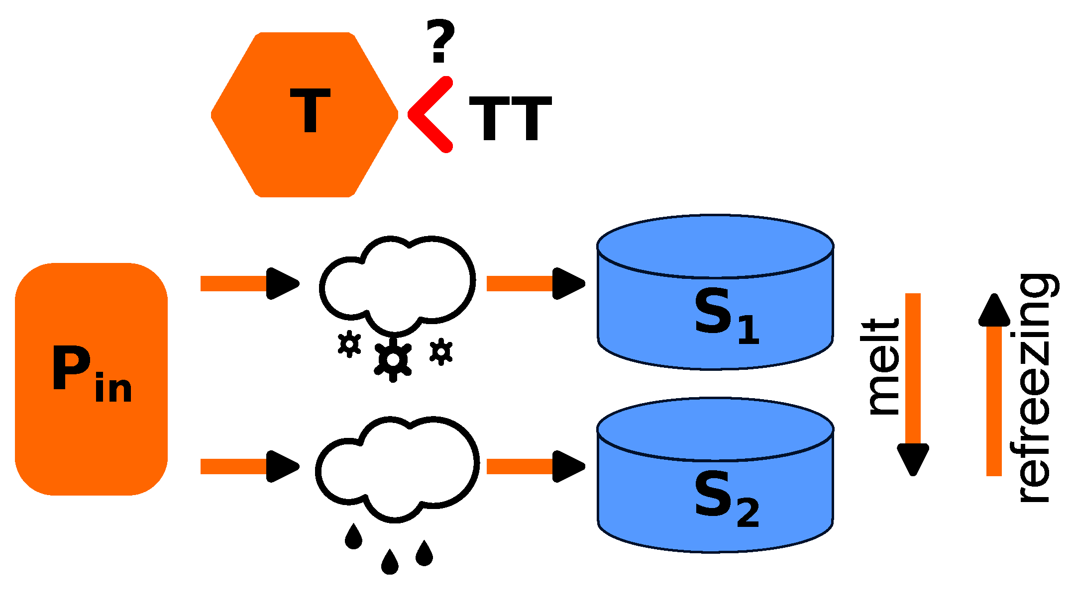
The HBV model has undergone improvements, with a commonly used version being HBV-96 [24]. This conceptual hydrologic runoff model simulates discharge using precipitation, temperature, and potential evaporation estimates. It consists of routines for snowfall, groundwater, evaporation, and runoff routing, utilizing a triangular-shaped weighting function. A schematic representation of the snow model relationships is shown in Figure 2. The model algorithm separates incoming precipitation ( P i n ) into liquid and solid based on ambient temperature, with solid precipitation falling into the snow storage reservoir ( S 1 ), and rain entering the liquid water reservoir ( S 2 ). An exchange of liquid occurs between these reservoirs through the melting of snow and the freezing of water.
Precipitation is classified as snow or rain depending on the temperature, which must be above or below the threshold temperature (TT). When the temperature falls below TT, all precipitation is considered snow. In such cases, the precipitation value is multiplied by the snowfall correction factor (SFCF), a parameter that accounts for systematic errors in snowfall measurements and evaporation from the snowpack that is not represented in the model. The degree-day method is employed to simulate snowmelt [24]
m e l t = C F M A X · T ( t ) T T .
Meltwater and precipitation are retained within the snowpack until they exceed a certain fraction of the snow water equivalent CWH. Liquid water in the snowpack refreezes according to the refreezing coefficient CFR [24]
r e f r e e z i n g = C F R · C F M A X · T T T ( t ) ,

3. Study Area

The Suunduk River catchment, a 174 km long river that serves as the first major tributary of the Ural in the Orenburg Region, offers a suitable case study for selecting an optimal conceptual model. The river originates from the eastern slope of the Southern Urals and flows through a region characterized by granite intrusions. Its lower reaches have an average annual discharge of approximately 4.00 m3/s, indicating a moderate-to-high level of hydrological activity in the area.
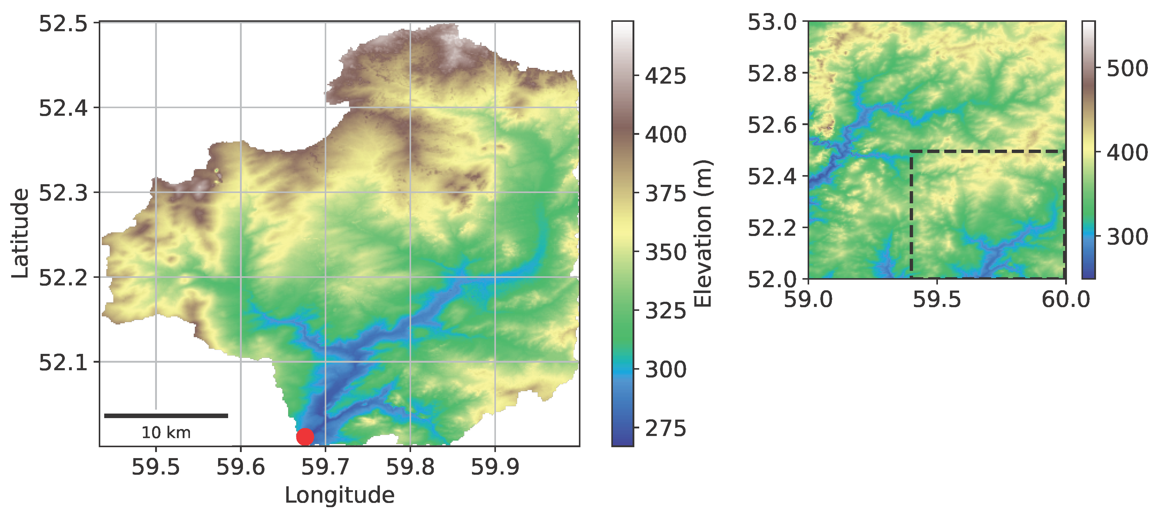
The river is marked by a high variability of annual runoff, with a coefficient of variation ranging from 0.82 to 1.0. Additionally, the coefficient of asymmetry of annual runoff is 1.8. The total area of the catchment under consideration is 4061.8 km2, and its average slope is 1.1‰. With an average height of 340 m, the altitudinal composition of the region can be visualized in the DEM (Figure 3). The natural zones are primarily forest steppe and steppe, which characterize the phases of the runoff regime. Spring floods account for 85–96% of the total annual runoff, with flood duration varying from 20 days. In contrast, summer–autumn runoff constitutes only 3–10% of the annual runoff, whereas winter runoff is noticeably less, depending on general moisture content and catchment regulating capacity, at approximately 1–4%.
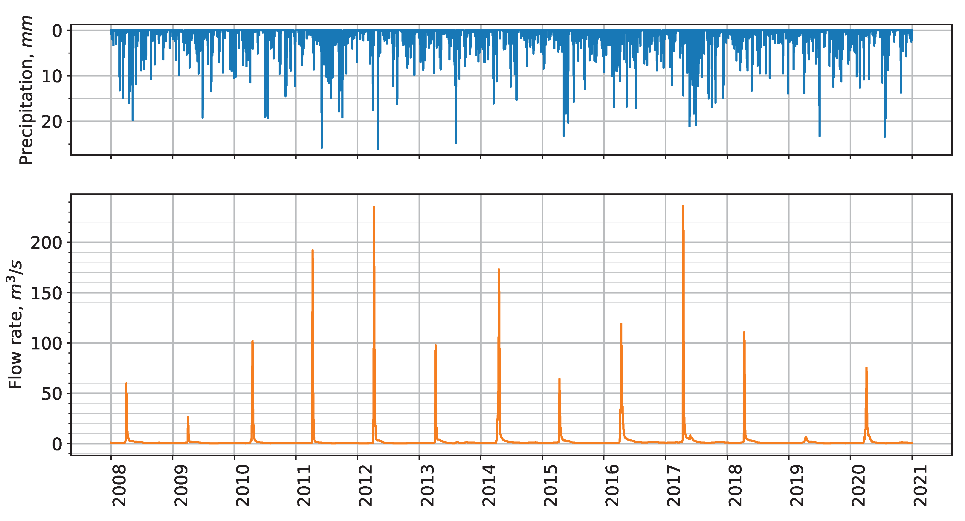
The accuracy of forecasts is significantly affected by the length of meteorological observation data and recorded flow data. A 12-year dataset from 1 January 2008 to 1 January 2020 for the considered catchment contains both meteorological parameters and river flow rate data, as presented in Figure 4. Forecast models are expected to underestimate runoff values in such case, a finding consistent with previous studies. In the work [32], the authors divided a 64-year observation period into subsets of different lengths (2, 5, 10, 20, and 30 years) to examine their impact on annual runoff forecasting. The results showed similar error ranges for both 2- and 5-year calibration data for each percentile, with significant reduction in overestimation when at least 10 years of calibration data were available. However, underestimation remained high even with 20 years of recorded flow rate data.
Additionally, the river bed is straight, resistant to erosion, and overgrown with aquatic vegetation. Bushes are found along the banks. The bottom is composed of a sandy–silty mixture, with rocky formations on the riffles. During periods of low water, the river bed transforms into a network of lake-like expansions where the water is practically stagnant. The depth of the water varies significantly across different sections, reaching up to 1.5–2.0 m on the riffles and only 0.2–0.5 m on the reaches.

4. Results and Discussion

4.1. Atmospheric Circulation Influence

The relationship between atmospheric circulation and runoff has also been explored in previous studies [33,34,35], including one on spring flooding due to snow melting [33]. Research found that warming associated with atmospheric circulation is linked to an increase in high geopotential anomalies in Northeastern North America during the considered period. Changes in weather regimes had a less clear impact on streamflow during the warm season, whereas temperature played a larger role in winter by altering the snow ratio and the snowmelt period. Consequently, it was determined that 40% of the increase in streamflow between December and March and a 45% decrease in streamflow in April were influenced by atmospheric circulation.
The inclusion of atmospheric circulation anomaly factors as supplementary training data has been explored in [34] to enhance the prediction accuracy and stability of runoff models, particularly during extreme weather periods. A similar approach was adopted in [35], where machine learning methods, including principal component analysis (PCA), were applied to determine the main factors influencing forecast from 130 atmospheric circulation indexes. The original monthly runoff series was also processed using variational mode decomposition (VMD) to extract stationary components. Notably, the rainfall–runoff process is closely connected to climatic conditions and human activities in addition to traditional meteorological factors such as precipitation and potential evapotranspiration. It has been suggested that atmospheric circulation indexes can comprehensively enhance the prediction performance of runoff models, including VMD-LSTM. This may be attributed to their long-term continuous influence on regional climate, which affects the climate for a prolonged period in the future and subsequently impacts runoff through the water cycle process.
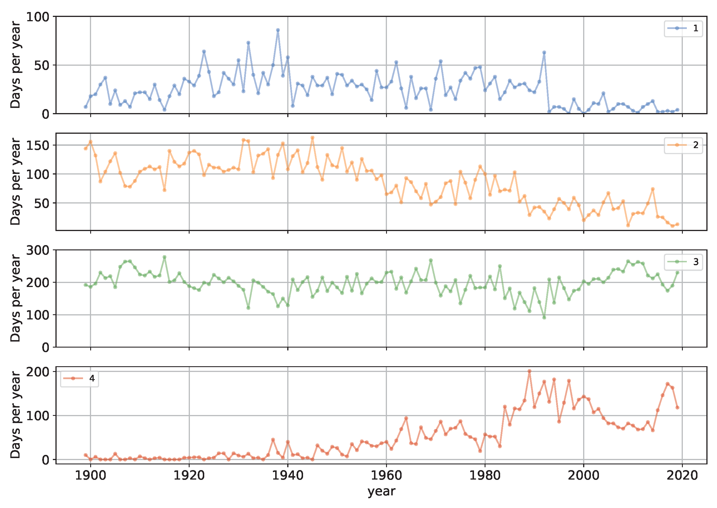
In this study, atmospheric circulation was categorized using the system developed by B. L. Dzerdzeevskii [36,37,38], which classifies atmospheric processes in the Northern Hemisphere based on Elementary Circulation Mechanisms (ECMs). This method relies on an analysis of large datasets of baric topography maps at the 500 hPa level. By examining these data, specific patterns were identified and used to highlight specific ECMs according to atmospheric pressure values, the quantity of arctic incursions per hemisphere, and their direction. The 41 ECM subtypes were further consolidated into 13 main types based on shared characteristics. In the European sector of the Northern Hemisphere, where the studied catchment area is located, the observed circulation types are grouped into four broad categories: west zonal, northern meridional, southern meridional, and a combination of west zonal and southern meridional, designated as groups 1 through 4, respectively.
Complete macro-level water cycles span the periods from 1950 to 1985 and from 1986 to 2000, each lasting 35 years. The high-water phases occurred from 1950 to 1972 (22 years) and from 1985 to 2002 (17 years), while the low-water phases were from 1973 to 1984 (11 years) and from 2000 to 2020 (20 years). It is important to emphasize that when developing runoff forecasting methods or evaluating flood runoff models, the calculation period should not be limited to either the low-water or high-water phases. Additionally, using only periods of low or high water levels, or varying periods of water content, for model verification and calibration is inappropriate [16,17]. Therefore, careful consideration of these factors is essential during the further calibration of hydrological models.
The hypothesis is that the formation of spring flood runoff in the Suunduk River is based on the following assumptions:
  • Snow accumulation primarily occurs when moisture-laden air masses from the North Atlantic move into the region, corresponding to ECM types 1 and 2;
  • The most significant soil freezing takes place during the influx of Arctic air masses and the development of anticyclones;
  • The highest levels of preceding autumn moisture, which influence soil moisture content and the formation of runoff losses due to infiltration during the snowmelt period, are associated with zonal circulation patterns (types 1–7)—in contrast, the lowest levels occur during the movement of air masses from Central Asia as well as from the Arctic (types 8–13).
The average duration of the enlarged ECM groups is presented in Figure 5, which makes it possible to assess their influence on the general circulation of the atmosphere in extratropical latitudes.
The proposed hypothesis was tested by conducting a series calculation to examine the relationship between atmospheric circulation and precipitations:
  • In order to establish a correlation between circulation patterns and autumn precipitation, this study analyzed the frequency of each circulation group during September–October.
  • To investigate the relationship between snow reserve amounts and different circulation patterns, the frequency of each circulation group for November–December and January–March is analyzed.
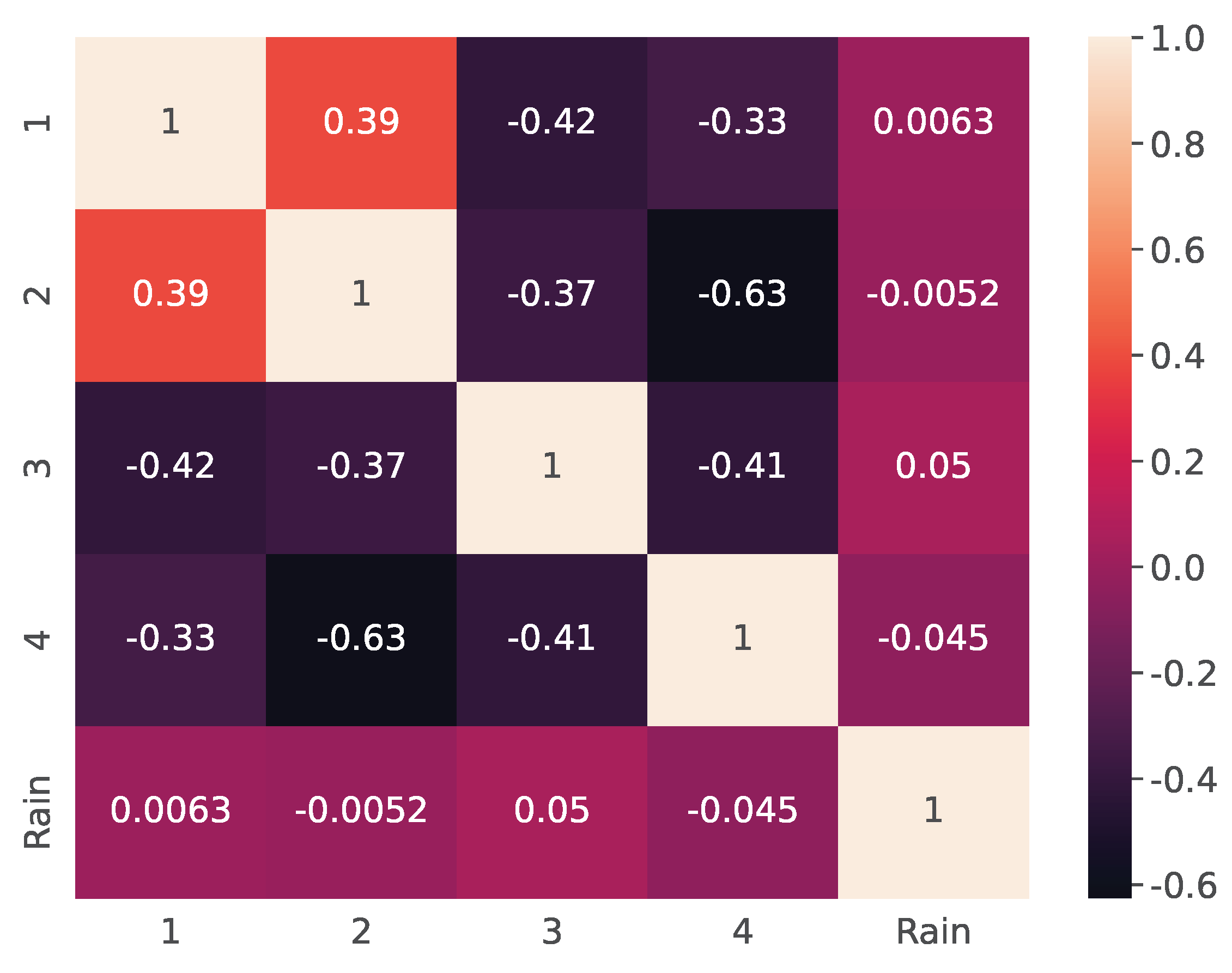
The correlation between the preceding autumn moisture and the frequency of atmospheric circulation groups is presented in Figure 6.
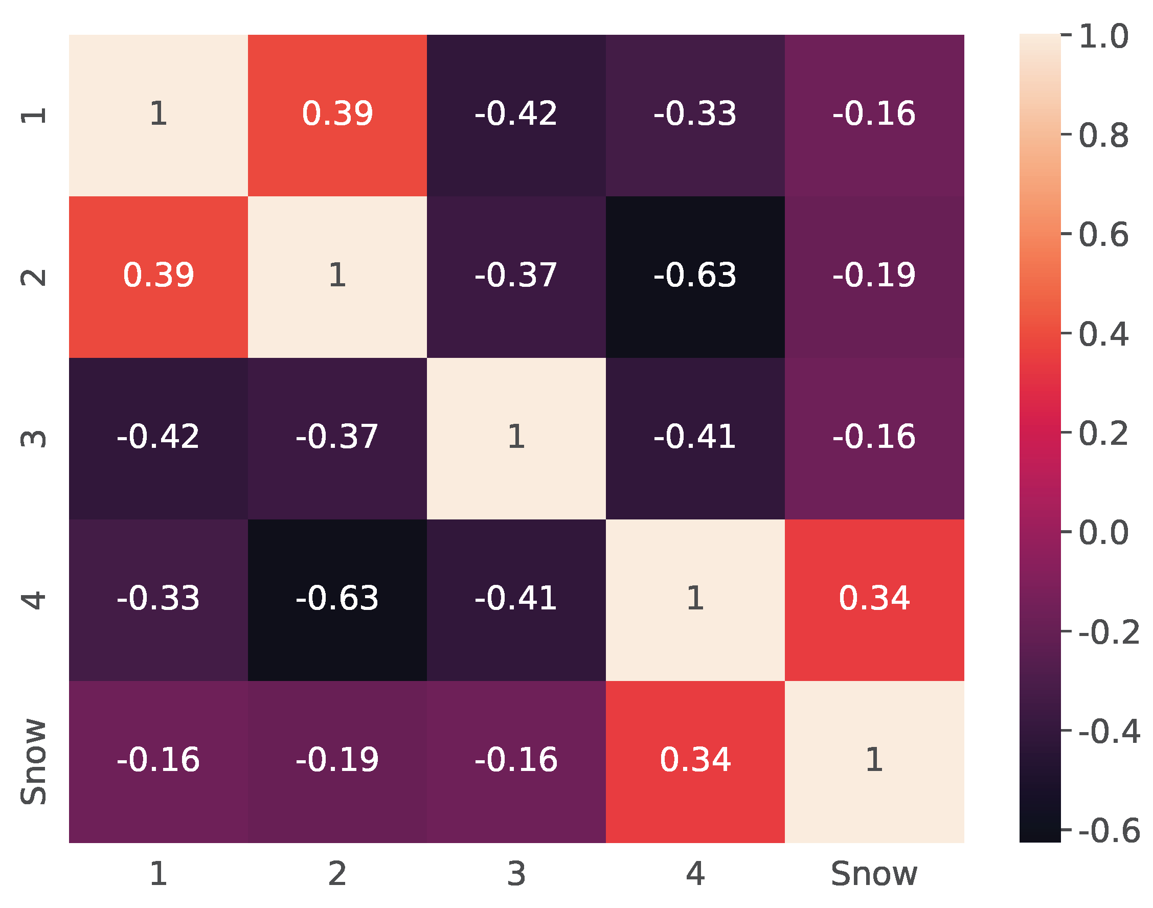
Figure 7 shows correlation between the amount of snow reserves and the frequency of different circulation groups.
The analysis of research findings did not support the hypothesis that ECM values are stably connected to primary factors influencing spring flood runoff in the Suunduk River basin. Although key contributing factors to spring flood runoff were identified, no consistent relationships between these factors and ECM values were detected. This lack of correlation undermines the theoretical basis for long-term forecasting of spring flood runoff at the hydroelectric power plant reservoir section with the help of ECMs. However, it is possible that the limited time range considered may have contributed to this lack of correlation, potentially obscuring additional relationships between atmospheric circulation patterns and spring runoff. Unfortunately, exploring an extended time range is not feasible at this stage due to data unavailability.

4.2. Strategy for Conceptual Model Setup

The final indicators of the accuracy of the modeling are affected by numerous factors, including uncertainty in the measured values, spatial density of meteorological stations, and length of retrospective data [3,21,22,23,24,25,26,27,28]. These factors exert a decisive impact on the obtained result. However, it is not possible to influence most of the presented factors during modeling, for instance, the length of retrospective data. Therefore, at this stage of the study, an assessment is made of how data preprocessing and the selected modeling efficiency metrics can affect the accuracy of modeling.
The results presented below illustrate the influence of the chosen objective function on the calibration process of the GR6J-CemaNeige model. The evaluation of all modeling strategies is primarily based on the most critical project parameter: the volume of runoff during the spring flood period, as defined by dependencies (3)–(5). The objective function employs metrics such as NSE (1) and KGE (2) as foundational elements. Figure 8 presents a comparison of relative errors in total runoff during the flood. In addition to single-metric objective functions, this study also explored multi-metric approaches that incorporate multiple performance metrics with adjustable weighting coefficients. Specifically, three different objective function configurations were considered, each weighing the contribution of two metrics differently: (1) NSE at 70% and KGE at 30%, (2) NSE at 50% and KGE at 50%, and (3) NSE at 30% and KGE at 70%.
Based on these results, it can be inferred that utilizing composite objective functions does not lead to a decrease in relative modeling error; instead, the most accurate result is achieved by employing an objective function based solely on the NSE metric.
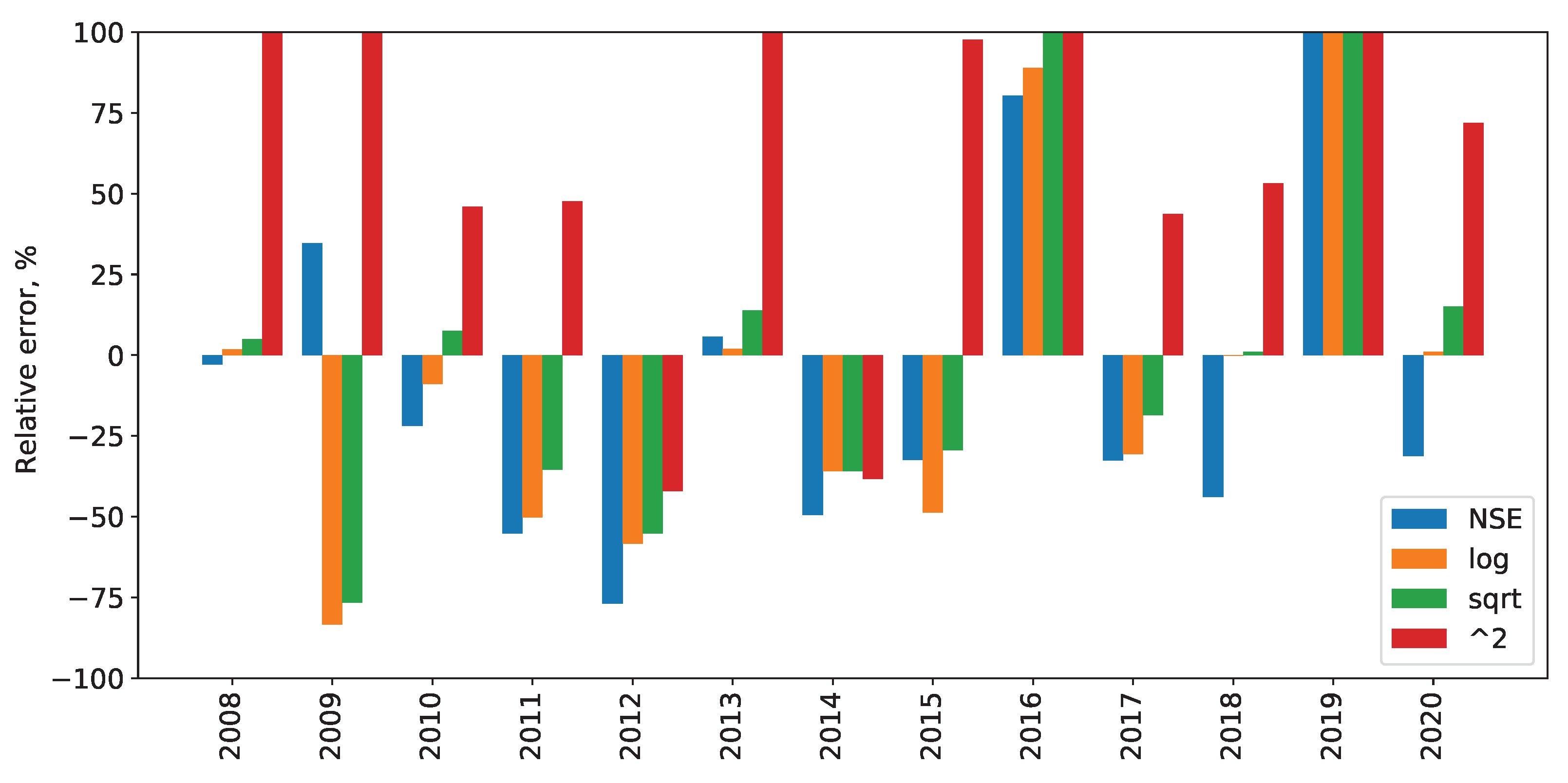
In addition to modifying the objective functions, transforming the runoff values has a significant impact that can improve the accuracy of the modeling in some cases. This is because by changing the original values, for example, by squaring or taking the square root, it is possible to either amplify some peak values or, conversely, reduce their influence when calibrating the model. Applying different mathematical functions to the runoff data can have a substantial effect on the modeling accuracy. Consider the following transformations of the runoff values: applying the natural logarithm function, taking the square root, and squaring. A comparison with the observed runoff is shown in Figure 9.
A baseline approach combining the square root function with the NSE metric has been established to enhance modeling accuracy. The impact of varying effective catchment areas on modeling accuracy was further investigated by applying coefficients of 2, 1, 0.5, 0.25, and 0.1. Results from this analysis are presented in Figure 10.
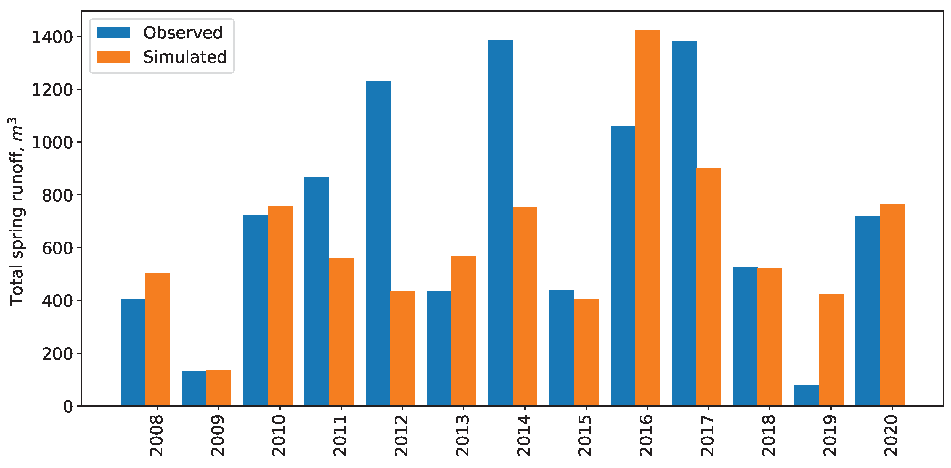
Our analysis indicates that applying a correction factor to the catchment area equal to 0.25 generally reduces the average error of modeling for most considered years. Therefore, using the NSE metric as a target function with runoff transformation by the square root function and applying a correction factor to the catchment area equal to 0.25 is an optimal approach for obtaining the results in the GR6J-CemaNeige model. The absolute values of this approach are presented in Figure 11.
In this study, another conceptual model HBV is considered. As previously described in Section 2, this model has a different structure and snow model. Due to its distinct architecture, the obtained results may differ from those of the GR6J-CemaNeige model. However, as the employed data preprocessing strategy increased accuracy when used with GR6J-CemaNeige, the same approach is applied to HBV. The resulting values are presented in Figure 12.
Comparing the two adjusted models by relative error (Figure 13) reveals discrepancies between their outcomes, with some years exhibiting errors of opposite signs. This observation suggests a potential complementarity between the two models. A study was conducted to explore the combined use of both models in different proportions, and the average relative error for the considered period was calculated alongside previously obtained results. The summarization of the average relative error is presented in Table 1.
Absolute values of total runoff during the flood period for the combined use of models in the ratio of 80% GR6J-CN and 20% HBV are presented in Figure 14.

4.3. Discussion

The simulated discharge values tend to underestimate peak discharges (Figure 11 and Figure 12), which may be attributed to insufficient observation density of meteorological parameters. This issue is further supported by a similar conclusion reached in a previous study that investigated the effect of the interpolation of precipitation in space using various spatial gauge densities on rainfall–runoff model discharge [39]. The study employed a physically based reference model with reconstructed precipitation as input and found that low spatial density led to a more frequent high underestimation of areal precipitation, especially for large events. Furthermore, using precipitation with no spatial variability resulted in an overall loss of model performance, particularly for events involving snowmelt. These findings highlight the primary issue associated with the low spatial density of observed parameters.
Implementing data assimilation (DA) techniques [40,41,42,43] can significantly improve predictions in hydrologic systems. DA is a crucial method that combines observations with physical constraints to enhance state estimates in dynamic systems. In hydrologic DA, various methods are commonly employed, including Kalman filtering, particle filtering, and variational DA [40,41]. Among these, the ensemble Kalman filter (EnKF) has emerged as an effective alternative to traditional Kalman filtering, particularly suitable for high-dimensional nonlinear problems. The EnKF updates state estimates recursively in time, making it ideal for real-time applications. Research has shown that EnKF-based DA techniques can improve model state estimates and forecasting accuracy in various fields, including hydrology and meteorology [40]. In contrast, particle filtering (PF), another popular technique, updates particle weights and states recursively as new observations become available. However, its implementation is complicated by the degeneracy problem [40]. Comparative studies have suggested that EnKF may outperform PF in short-term applications [42], while PF-based estimates may have a longer-lasting updating effect when accounting for both meteorological and state uncertainties. A comparative analysis of EnKF and PF in streamflow forecasting highlighted the importance of routing dynamics and accurate estimation of forecast initial conditions. The results showed that, although EnKF-based estimates may be more efficient in the short term, PF-based estimates can provide a longer-lasting updating effect when considering both meteorological and state uncertainties [42].
The models were calibrated over the entire time interval, encompassing various climatic conditions. This calibration process ensures that the model achieves its highest accuracy for the parameters most frequently encountered within the period under consideration. Such an approach might affect accuracy in unforeseen situations. An illustrative example of such a problem can be found in the study [44], where a differential split-sample test was employed to evaluate the transferability of model parameters across different hydroclimate conditions The findings indicated that parameterization approaches focusing on consistent performance during both dry and wet periods can effectively reproduce observed runoff for historical periods, albeit without necessarily yielding more reliable future projections. Nonetheless, ensemble simulations based on diverse parameterization considerations can produce a broader range of projections by accounting for uncertainties stemming from model parameters.
The parameters for both models (GR and HBV) are listed in Table 2 and Table 3. The comparison of the calibrated values reveals significant differences between similar parameters. Specifically, the degree-day factor for snowmelt differs by 20% and the time constant by 26.4% compared to the GR model. These discrepancies arise from distinct water routing mechanisms employed in each model. Notably, these differences have not had a proportional impact on final accuracy. This might be attributed to limitations in the used data, as previously discussed.
Combining machine learning tools with conceptual models is a promising approach, particularly in cases where meteorological conditions differ significantly from those used to obtain optimal model parameters. This was explored in a study [45] that compared a conceptual model and a neural network (NN) model to simulate discharge and piezometry of a karst aquifer. Both models demonstrated satisfactory performance on test sets specific to discharge and groundwater levels. However, the NN model outperformed the conceptual model in flash flood simulations, while the conceptual model excelled in simulating intermediate high-water levels in spring. Conversely, the NN model was more effective in simulating drawdown, and the conceptual model was preferred for aquifer recharge simulations, indicating that the models are complementary. The conceptual model showed improvement when accompanied by an a priori estimate of evapotranspiration, suggesting its effectiveness in contexts with limited measurement data. The NN model’s capacity to learn the nonlinearity of karst aquifers suggests its potential for flood or drought forecasting. Another study [46] investigated a hybrid model for spring discharge prediction, combining a conceptual GR5J lumped model with a machine learning random forest (RF) algorithm. This hybrid model, which integrated both physical knowledge and pattern recognition capabilities, achieved an error reduction of approximately 25% compared to the conceptual model alone and 55% compared to the ML model alone. However, the performance of the hybrid model depends on the accuracy of both components, as errors in the conceptual model can propagate through the hybrid model. The study also emphasized the importance of accounting for meteorological input uncertainty using ensemble forcing to improve predictive accuracy when actual inputs are unknown.

5. Conclusions

In conclusion, this study aimed to enhance the accuracy of runoff forecasts for reservoirs during the spring flood period in forest steppe and steppe natural zones. By focusing on the total volume of water entering the reservoir rather than instantaneous daily flow rates, the study prioritized the integral runoff value, which is crucial for hydroelectric power plant operations. Conceptual lumped models, specifically GR6J-CemaNeige and HBV, were employed to achieve this goal.
The research explored the potential of dynamic model parameters, which led to the exploration of a hypothesis linking atmospheric circulation patterns to dry and wet periods. However, the hypothesis that atmospheric circulation could predict these periods was not substantiated, highlighting the limitations of long-term forecasting models based on such correlations.
This study also underscored the impact of data quality on model performance, with significant deviations from observed data occurring in certain years, likely due to insufficient meteorological observation density. The results showed that while both models could be calibrated to perform reasonably well across various climatic conditions, their predictive accuracy might be compromised in unforeseen situations. The application of a correction factor to the catchment area and the use of the NSE metric with runoff transformation were identified as effective strategies for improving model accuracy.
Despite these advancements, the average relative error of approximately 25% observed in this study indicates that further refinement is necessary. Overall, this research contributes to the understanding of hydrological modeling in steppe regions, offering insights into both the capabilities and limitations of current approaches. These findings are essential for the ongoing development of more accurate and reliable forecasting models, which are critical for effective water resource management and sustainable energy production in hydroelectric power plants.

Author Contributions

Conceptualization, S.E. and E.S.; formal analysis, S.E., E.S. and D.K.; investigation, E.S. and I.I.; writing—original draft preparation, E.S.; visualization, E.S. and I.I.; writing—review and editing, E.S. and S.E; supervision, S.E. and D.K. All authors have read and agreed to the published version of the manuscript.

Funding

The research was carried out within the state assignment with the financial support of the Ministry of Science and Higher Education of the Russian Federation (subject No. FEUZ-2022-0030 Development of an intelligent multi-agent system for modeling deeply integrated technological systems in the power industry).

Institutional Review Board Statement

Not applicable.

Data Availability Statement

The data presented in this study are available on request from the corresponding author due to privacy restrictions.

Conflicts of Interest

The authors declare no conflicts of interest.

References

  1. Dalla Torre, D.; Di Marco, N.; Menapace, A.; Avesani, D.; Righetti, M.; Majone, B. Suitability of ERA5-Land reanalysis dataset for hydrological modelling in the Alpine region. J. Hydrol. Reg. Stud. 2024, 52, 101718. [Google Scholar] [CrossRef]
  2. Vasil’ev, D.; Vodopyanov, V.; Zayzeva, G.; Zakirzyanov, S.; Semenov, V.; Sivokhip, Z.; Chibilev, A. Long-term forecast model of spring runoff on the Belaya river. Dokl. Earth Sci. 2019, 486, 723–726. [Google Scholar] [CrossRef]
  3. Valery, A.; Andreassian, V.; Perrin, C. As simple as possible but not simpler: What is useful in a temperature-based snow-accounting routine? Part 2 – Sensitivity analysis of the Cemaneige snow accounting routine on 380 catchments. J. Hydrol. 2014, 517, 1176–1187. [Google Scholar] [CrossRef]
  4. Zaramella, M.; Borga, M.; Zoccatelli, D.; Carturan, L. TOPMELT 1.0: A topography-based distribution function approach to snowmelt simulation for hydrological modelling at basin scale. Geosci. Model Dev. 2019, 12, 5251–5265. [Google Scholar] [CrossRef]
  5. Di Marco, N.; Avesani, D.; Righetti, M.; Zaramella, M.; Majone, B.; Borga, M. Reducing hydrological modelling uncertainty by using MODIS snow cover data and a topography-based distribution function snowmelt model. J. Hydrol. 2021, 599, 126020. [Google Scholar] [CrossRef]
  6. Magnusson, J.; Nævdal, G.; Matt, F.; Burkhart, J.F.; Winstral, A. Improving hydropower inflow forecasts by assimilating snow data. Hydrol. Res. 2020, 51, 226–237. [Google Scholar] [CrossRef]
  7. Khalyasmaa, A.; Eroshenko, S.; Mazunina, M. Prospects for the Use of Intelligent Multi-agent Models for the Control of Objects of Deeply Integrated Power Systems. In Proceedings of the 2022 IEEE International Multi-Conference on Engineering, Computer and Information Sciences (SIBIRCON), Yekaterinburg, Russia, 11–13 November 2022; pp. 730–733. [Google Scholar] [CrossRef]
  8. Eroshenko, S.; Matrenin, P.; Khalyasmaa, A.; Klimenko, D.; Sidorova, A. Data Processing Technology for the Forecasting of the Water Inflow into a Reservoir with the Use of Earth Remote Sensing and the Network of Meteorological and Hydrological Posts. Probl. Reg. Energetics 2022, 56, 100–109. [Google Scholar] [CrossRef]
  9. Hawker, L.; Bates, P.; Neal, J.; Rougier, J. Perspectives on Digital Elevation Model (DEM) Simulation for Flood Modeling in the Absence of a High-Accuracy Open Access Global DEM. Front. Earth Sci. 2018, 6, 233. [Google Scholar] [CrossRef]
  10. Woldegebrael, S.M.; Kidanewold, B.B.; Melesse, A.M. Seasonal Flow Forecasting Using Satellite-Driven Precipitation Data for Awash and Omo-Gibe Basins, Ethiopia. Remote Sens. 2022, 14, 4518. [Google Scholar] [CrossRef]
  11. Matrenin, P.; Safaraliev, M.; Kiryanova, N.; Sultonov, S. Monthly Runoff Forecasting by Non-Generalizing Machine Learning Model and Feature Space Transformation (Vakhsh River Case Study). Probl. Reg. Energetics 2022, 55, 99–110. [Google Scholar] [CrossRef]
  12. Klimenko, D. Estimating the Probable Maximum Precipitation by Physical Methods Using Satellite and Radiolocation Observation Data: Case Study of the Middle Urals. Water Resour. 2020, 47, 443–452. [Google Scholar] [CrossRef]
  13. Susilowati, Y.; Irasari, P.; Kumoro, Y.; Hendriawan Nur, W.; Yunarto, Y. Micro hydropower plant potential study based on Landsat 8 operational land imager satellite data. Bull. Electr. Eng. Inform. 2021, 10, 3167–3177. [Google Scholar] [CrossRef]
  14. Udnæs, H.C.; Alfnes, E.; Andreassen, L.M. Improving runoff modeling using satellite-derived snow cover area. Water Policy 2007, 38, 21–32. [Google Scholar] [CrossRef]
  15. Kochendorfer, J.; Earle, M.; Rasmussen, R.; Smith, C.; Yang, D.; Morin, S.; Mekis, E.; Buisan, S.; Roulet, Y.A.; Landolt, S.; et al. How Well are We Measuring Snow Post-SPICE? Bull. Am. Meteorol. Soc. 2021, 103, E370–E388. [Google Scholar] [CrossRef]
  16. Watson, A.; Midgley, G.; Ray, P.; Kralisch, S.; Helmschrot, J. How Climate Extremes Influence Conceptual Rainfall-Runoff Model Performance and Uncertainty. Front. Clim. 2022, 4, 859303. [Google Scholar] [CrossRef]
  17. Stephens, C.; Marshall, L.; Johnson, F. Investigating strategies to improve hydrologic model performance in a changing climate. J. Hydrol. 2019, 579, 124219. [Google Scholar] [CrossRef]
  18. Astagneau, P.C.; Thirel, G.; Delaigue, O.; Guillaume, J.H.A.; Parajka, J.; Brauer, C.C.; Viglione, A.; Buytaert, W.; Beven, K.J. Technical note: Hydrology modelling R packages—A unified analysis of models and practicalities from a user perspective. Hydrol. Earth Syst. Sci. 2021, 25, 3937–3973. [Google Scholar] [CrossRef]
  19. Devia, G.; Bigganahalli Puttaswamigowda, G.; Dwarakish, G. A Review on Hydrological Models. Aquat. Procedia 2015, 4, 1001–1007. [Google Scholar] [CrossRef]
  20. Yaduvanshi, A.; Srivastava, P.; Worqlul, A.W.; Sinha, A.K. Uncertainty in a Lumped and a Semi-Distributed Model for Discharge Prediction in Ghatshila Catchment. Water 2018, 10, 381. [Google Scholar] [CrossRef]
  21. Gao, C.; He, Z.; Pan, S.; Weidong, X.; Xu, Y. Effects of climate change on peak runoff and flood levels in Qu River Basin, East China. J. -Hydro-Environ. Res. 2018, 28, 34–47. [Google Scholar] [CrossRef]
  22. Neri, M.; Parajka, J.; Toth, E. Importance of the informative content in the study area when regionalising rainfall-runoff model parameters: The role of nested catchments and gauging station density. Hydrol. Earth Syst. Sci. 2020, 24, 5149–5171. [Google Scholar] [CrossRef]
  23. Bergstrom, S. Development and Application of a Conceptual Runoff Model for Scandinavian Catchments; SMHI Rapporter: Norrkoping, Sweden, 1976; Volume 134. [Google Scholar]
  24. Lindstrom, G.; Johansson, B.; Persson, M.; Gardelin, M.; Bergstrom, S. Development and test of the distributed HBV-96 hydrological model. J. Hydrol. 1997, 201, 272–288. [Google Scholar] [CrossRef]
  25. Pianosi, F.; Wagener, T. A simple and efficient method for global sensitivity analysis based on cumulative distribution functions. Environ. Model. Softw. 2015, 67, 1–11. [Google Scholar] [CrossRef]
  26. Pianosi, F.; Beven, K.; Freer, J.; Hall, J.; Rougier, J.; Stephenson, D.; Wagener, T. Sensitivity analysis of environmental models: A systematic review with practical workflow. Environ. Model. Softw. 2016, 79, 214–232. [Google Scholar] [CrossRef]
  27. Moriasi, D.; Arnold, J.; Van Liew, M.; Bingner, R.; Harmel, R.; Veith, T. Model Evaluation Guidelines for Systematic Quantification of Accuracy in Watershed Simulations. Trans. ASABE 2007, 50, 885–900. [Google Scholar] [CrossRef]
  28. Ochoa-Tocachi, B.; Cuadros Adriazola, J.E.; Arapa, E.; Aste, N.; Ochoa-Tocachi, E.; Bonnesoeur, V. Guide to Hydrologic Modeling of Natural Infrastructure; Forest Trends: Lima, Peru, 2022. [Google Scholar] [CrossRef]
  29. Nash, J.; Sutcliffe, J. River flow forecasting through conceptual models part I — A discussion of principles. J. Hydrol. 1970, 10, 282–290. [Google Scholar] [CrossRef]
  30. Gupta, H.V.; Kling, H.; Yilmaz, K.K.; Martinez, G.F. Decomposition of the mean squared error and NSE performance criteria: Implications for improving hydrological modelling. J. Hydrol. 2009, 377, 80–91. [Google Scholar] [CrossRef]
  31. Majone, B.; Avesani, D.; Zulian, P.; Fiori, A.; Bellin, A. Analysis of high streamflow extremes in climate change studies: How do we calibrate hydrological models? Hydrol. Earth Syst. Sci. 2022, 26, 3863–3883. [Google Scholar] [CrossRef]
  32. Boughton, W. Effect of data length on rainfall-runoff modeling. Environ. Model. Softw. 2007, 22, 406–413. [Google Scholar] [CrossRef]
  33. Champagne, O.; Arain, M.; Coulibaly, P. Atmospheric circulation amplifies shift of winter streamflow in Southern Ontario. J. Hydrol. 2019, 578, 124051. [Google Scholar] [CrossRef]
  34. Yan, X.; Chang, Y.; Yang, Y.; Liu, X. Monthly runoff prediction using modified CEEMD-based weighted integrated model. J. Water Clim. Chang. 2020, 12, 1744–1760. [Google Scholar] [CrossRef]
  35. Wang, W.; Tang, S.; Zou, J.; Li, D.; Ge, X.; Huang, J.; Yin, X. Runoff Prediction in Different Forecast Periods via a Hybrid Machine Learning Model for Ganjiang River Basin, China. Water 2024, 16, 1589. [Google Scholar] [CrossRef]
  36. Malygina, N.; Papina, T.; Kononova, N.; Barlyaeva, T. Influence of atmospheric circulation on precipitation in Altai Mountains. J. Mt. Sci. 2017, 14, 46–59. [Google Scholar] [CrossRef]
  37. Lebedeva, M.G.; Lupo, A.R.; Chendev, Y.G.; Krymskaya, O.V.; Solovyev, A.B. Changes in the Atmospheric Circulation Conditions and Regional Climatic Characteristics in Two Remote Regions Since the Mid-20th Century. Atmosphere 2019, 10, 11. [Google Scholar] [CrossRef]
  38. Gorbunov, R.; Gorbunova, T.; Kononova, N.; Priymak, A.; Salnikov, A.; Drygval, A.; Lebedev, Y. Spatiotemporal aspects of interannual changes precipitation in the crimea. J. Arid. Environ. 2020, 183, 104280. [Google Scholar] [CrossRef]
  39. Bárdossy, A.; Anwar, F. Why do our rainfall–runoff models keep underestimating the peak flows? Hydrol. Earth Syst. Sci. 2023, 27, 1987–2000. [Google Scholar] [CrossRef]
  40. Liu, Y.; Gupta, H.V. Uncertainty in hydrologic modeling: Toward an integrated data assimilation framework. Water Resour. Res. 2007, 43. [Google Scholar] [CrossRef]
  41. Vrugt, J.A.; Robinson, B.A. Treatment of uncertainty using ensemble methods: Comparison of sequential data assimilation and Bayesian model averaging. Water Resour. Res. 2007, 43. [Google Scholar] [CrossRef]
  42. Piazzi, G.; Thirel, G.; Perrin, C.; Delaigue, O. Sequential Data Assimilation for Streamflow Forecasting: Assessing the Sensitivity to Uncertainties and Updated Variables of a Conceptual Hydrological Model at Basin Scale. Water Resour. Res. 2021, 57. [Google Scholar] [CrossRef]
  43. Lu, M.; Lu, S.; Liao, W.; Lei, X.; Yin, Z.; Wang, H. Research and application of parameter estimation method in hydrological model based on dual ensemble Kalman filter. Hydrol. Res. 2021, 53, 65–84. [Google Scholar] [CrossRef]
  44. Zheng, H.; Chiew, F.H.; Zhang, L. Can Model Parameterization Accounting for Hydrological Nonstationarity Improve Robustness in Future Runoff Projection? J. Hydrometeorol. 2022, 23, 1831–1844. [Google Scholar] [CrossRef]
  45. Kong-A-Siou, L.; Fleury, P.; Johannet, A.; Borrell Estupina, V.; Pistre, S.; Dörfliger, N. Performance and complementarity of two systemic models (reservoir and neural networks) used to simulate spring discharge and piezometry for a karst aquifer. J. Hydrol. 2014, 519, 3178–3192. [Google Scholar] [CrossRef]
  46. Bouhafa, N.; Sakarovitch, C.; Lalague, L.; Goulard, F.; Pryet, A. Hybrid modeling of karstic springs: Error correction of conceptual reservoir models with machine learning. Water Supply 2024, 24, 1559–1573. [Google Scholar] [CrossRef]
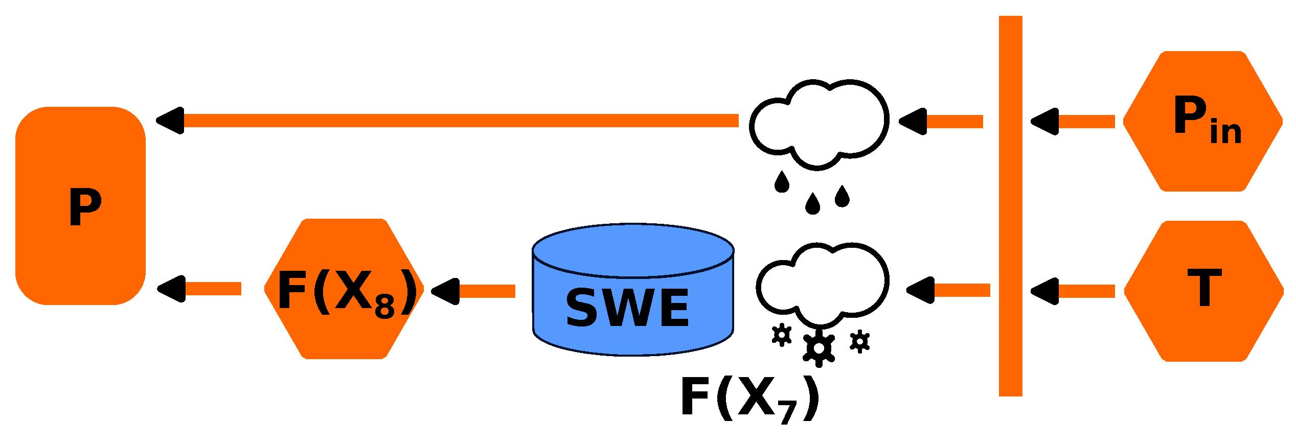
Figure 1. CemaNeige snow model block diagram.
Inventions 09 00109 g001
Figure 2. HBV snow model block diagram.
Inventions 09 00109 g002
Figure 3. Representation of catchment under study: the left side is the elevation distribution on the catchment view, with the outlet of catchment as a red dot; the right side is an extended view of the study area.
Inventions 09 00109 g003
Figure 4. Graph of time series precipitation and flow rate data.
Inventions 09 00109 g004
Figure 5. The timeline of the number of day per year for a particular atmospheric circulation group.
Inventions 09 00109 g005
Figure 6. Correlation values between the previous autumn moisture and the frequency of different groups of atmospheric circulation.
Inventions 09 00109 g006
Figure 7. Correlation values between the accumulated snow and the frequency of different groups of atmospheric circulation.
Inventions 09 00109 g007
Figure 8. The value of the modeling relative error when using different metrics (GR6J-CemaNeige).
Inventions 09 00109 g008
Figure 9. The value of the modeling relative error when using different flow rate transformation functions (GR6J-CemaNeige).
Inventions 09 00109 g009
Figure 10. The value of the modeling relative error when using different coefficients of effective catchment area (GR6J-CemaNeige).
Inventions 09 00109 g010
Figure 11. Results of the GR6J-CemaNeige model simulation in absolute values: on the left are the flow values, and on the right are the total runoff values during the flood period.
Inventions 09 00109 g011
Figure 12. Results of the HBV model simulation in absolute values: on the left are the flow values, and on the right are the total runoff values during the flood period.
Inventions 09 00109 g012
Figure 13. The value of the modeling relative error when using different conceptual models.
Inventions 09 00109 g013
Figure 14. Total runoff values during spring flood (results of combining two models).
Inventions 09 00109 g014
Table 1. Comparative table of data preprocessing method influence.
Modified Calibration ParameterParameter ValueAverage Relative Error Value, %
Metric usedNSE39
KGE41
30% NSE 70% KGE
50% NSE 50% KGE
70% NSE 30% KGE
Flow rate transformation functionNone39
Natural logarithm34
Square root33
Squaring94
Coefficient for catchment area235
133
0.530
0.2525
0.133
Models usedGR6J25
HBV28
80% GR6J-CN 20% HBV24
50% GR6J-CN 50% HBV25
20% GR6J-CN 80% HBV27
Table 2. GR model parameters.
ParameterDenotationUnitRange of Initial ValuesOptimal Values for Catchment under Study
Production store capacityX1mm36.6–90.0248.22
Intercatchment exchange coefficientX2mm/day(−1.17)–0.52−1.18
Routing store capacityX3mm27–15050
Unit hydrograph time constantX4day1.37–2.351.25
Intercatchment exchange thresholdX5(−0.18)–0.220.28
Exponential store depletion coefficientX6mm20.1–1508.45
Weighting coefficient for snow pack thermal stateX70–0.70.7
Degree-day melt coefficientX8mm/(C · day)3.8–6.84.96
Accumulation thresholdX9mm15–8550
Percentage (between 0 and 1) of annual snowfall defining the melt thresholdX100.15–0.850.17
Table 3. HBV model parameters.
ParameterDenotationUnitRange of Initial ValuesOptimal Values for Catchment under Study
Threshold temperature for snow and snowmeltTTC (−3)–1−0.2
Degree-day factor for snowmeltCFMAXmm/(C · day)0.06–103.93
Snowfall correction factorSFCF0.4–1.61
Refreezing coefficient for water in the snowpackCFR0.001–0.90.05
Liquid water holding capacity of the snowpackCWH0.001–0.90.2
Maximum percolation from upper to lower groundwater storagePERCmm/day0–30.59
Threshold for quick runoff for K0 outflowUZLmm0–10090
Recession coefficient (quick runoff)K00.001–0.50.17
Recession coefficient (upper groundwater storage)K10.0001–0.20.15
Recession coefficient (lower groundwater storage)K2(2 × 10⁻⁶)–0.0050.004
Routing, length of triangular weighting functionMAXBASday1–71.58
Maximum amount of soil moisture storageFCmm50–550124.5
Threshold for reduction in evaporationLP0.3–10.8
Shape coefficient in soil routineBETA1–53.5
Disclaimer/Publisher’s Note: The statements, opinions and data contained in all publications are solely those of the individual author(s) and contributor(s) and not of MDPI and/or the editor(s). MDPI and/or the editor(s) disclaim responsibility for any injury to people or property resulting from any ideas, methods, instructions or products referred to in the content.