
Multi-Objective Optimization of a Two-Stage Helical Gearbox Using MARCOS Method

 and
and
Abstract
1. Introduction
2. Optimization Problem
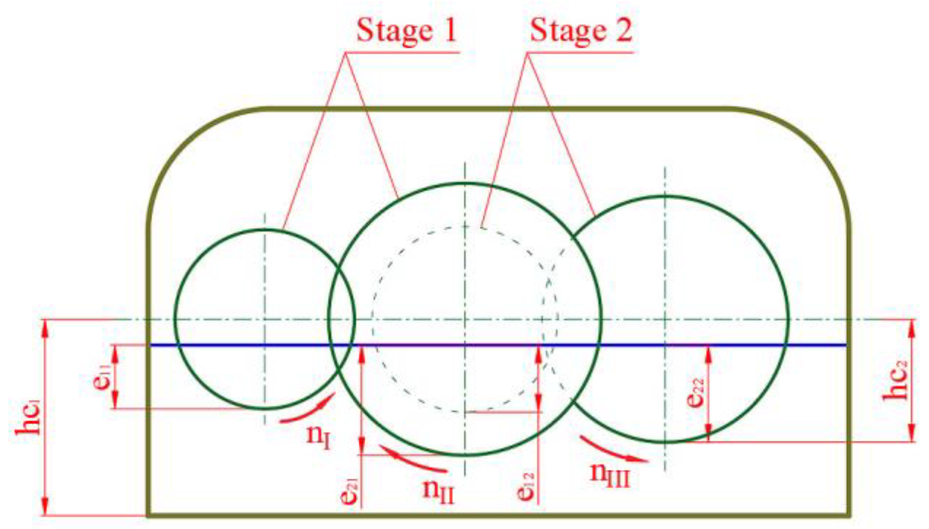
2.1. Calculation of Gearbox Volume
2.2. Calculation of Gearbox Efficiency
- -
- If v ≤ 0.424 (m/s),
- -
- If v > 0.424 (m/s),
2.3. Multi-Objective Optimization Problem
- -
- Minimizing the gearbox volume—
- -
- Maximizing the gearbox efficiency—
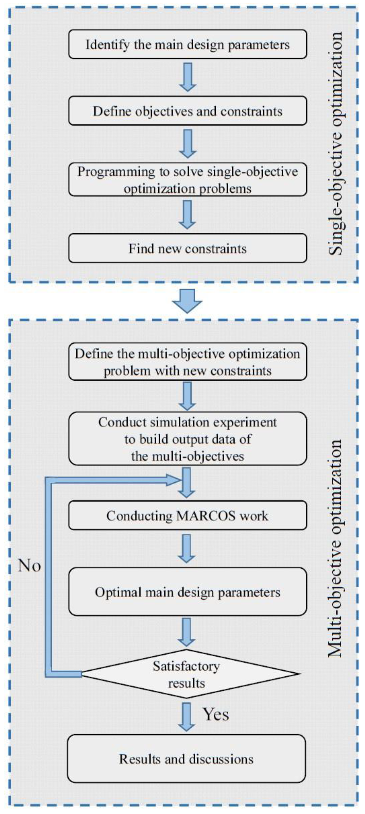
3. Methodology
3.1. Method to Solve the Multi-Objective Optimization
3.2. Method to Solve MCDM Problem
- -
- Making initial decision-making matrix
- -
- An extended initial matrix is produced by appending an ideal (AI) and anti-ideal solution (AAI) to the original decision-making matrix
- -
- One then normalizes the extended starting matrix (X). To calculate the normalized matrix , we use the following formula:
- -
- Determine the weighted normalized matrix by
- -
- Find the utility of alternatives Ki− and Ki+ by
- -
- Find the utility function f(Ki) of alternatives by
- -
- To determine which alternative has the highest utility function value, rank the options according to the final utility function values.
3.3. Method to Find the Weight of Criteria
- -
- Finding indicator-normalized values,
- -
- Calculating the Entropy for each indicator,
- -
- Determining the weight of each indicator,
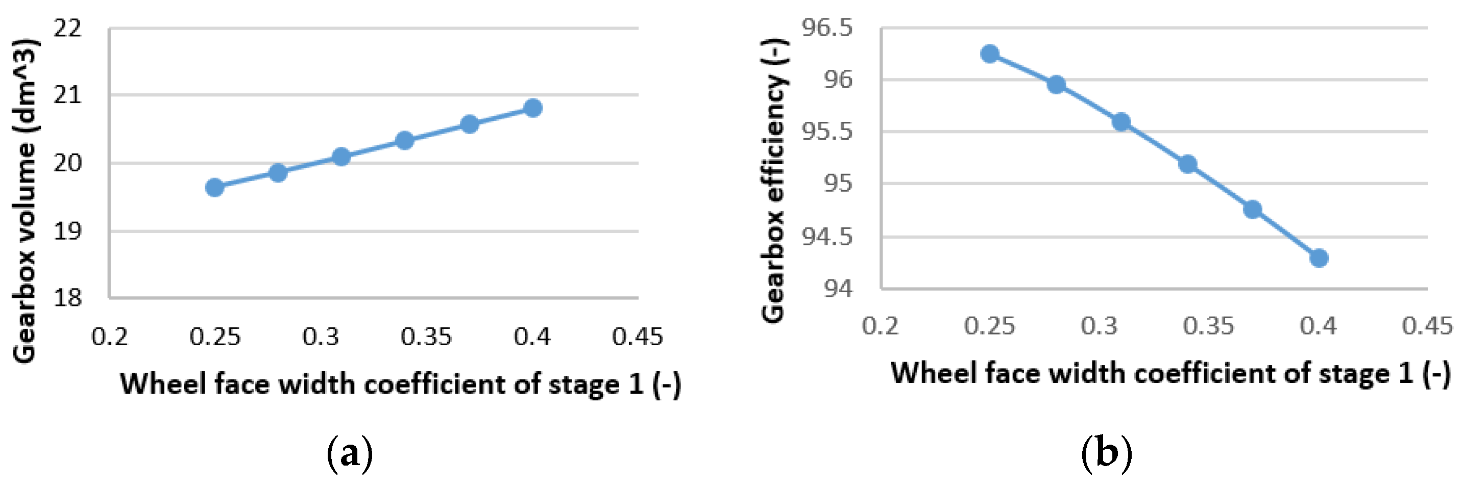
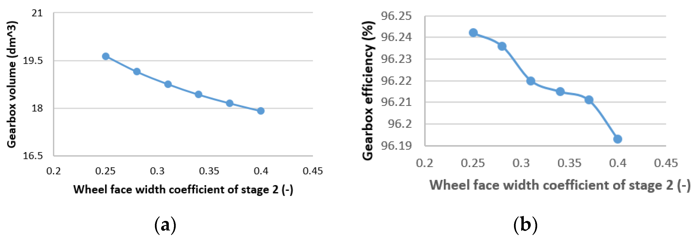
4. Single-Objective Optimization
5. Multi-Objective Optimization
6. Conclusions
- -
- The single-objective optimization problem speeds up and simplifies the resolution of the MOOP by bridging the gap between variable levels;
- -
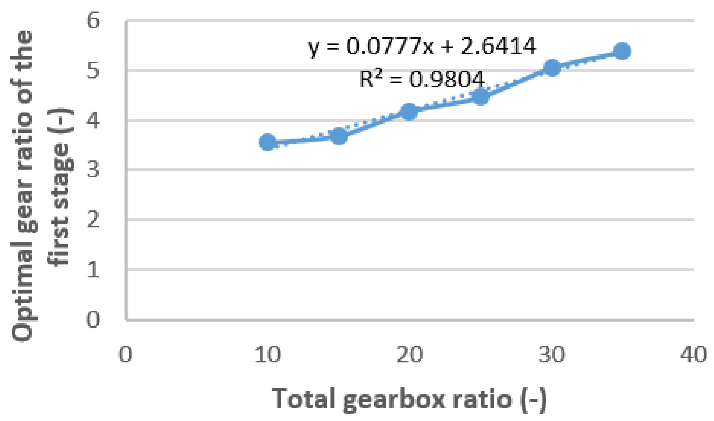
- The three main design parameters for a two-stage helical gear gearbox, Equation (51) and Table 6, were recommended to have optimal values based on the study’s findings;
- -
- In regard to the important design characteristics, two single objectives—the minimal gearbox volume and the greatest gear-box efficiency—were assessed;
- -
- By using the MARCOS technique repeatedly until the desired results are reached, the MOOP can be solved more precisely (u1 has an accuracy of less than 0.02);
- -
- The experimental data’s extraordinary degree of concordance with the proposed model of u1 verifies their reliability;
- -
- Further research is required to determine how to apply the proposed approach for solving the MOOP for various domains and MCDM methods.
Author Contributions
Funding
Data Availability Statement
Acknowledgments
Conflicts of Interest
References
- Pi, V.N. Optimal determination of partial transmission ratios for four-step helical gearboxes with first and third step double gear-sets for minimal mass of gears. In Proceedings of the WSEAS International Conference on Applied Computing Conference, Istanbul, Turkey, 27–30 May 2008. [Google Scholar]
- Golabi, S.I.; Fesharaki, J.J.; Yazdipoor, M. Gear train optimization based on minimum volume/weight design. Mech. Mach. Theory 2014, 73, 197–217. [Google Scholar] [CrossRef]
- Rai, P.; Agrawal, A.; Saini, M.L.; Jodder, C.; Barman, A.G. Volume optimization of helical gear with profile shift using real coded genetic algorithm. Procedia Comput. Sci. 2018, 133, 718–724. [Google Scholar] [CrossRef]
- Tamboli, K.; Patel, S.; George, P.; Sanghvi, R. Optimal design of a heavy duty helical gear pair using particle swarm optimization technique. Procedia Technol. 2014, 14, 513–519. [Google Scholar] [CrossRef]
- Khai, D.Q.; Linh, N.H.; Danh, T.H.; Tan, T.M.; Cuong, N.M.; Hien, B.T.; Pi, V.N.; Dung, N.T.Q. Calculating Optimum Main Design Factors of a Two-Stage Helical Gearboxes for Minimum Gearbox Mass. In International Conference on Engineering Research and Applications; Springer: Berlin/Heidelberg, Germany, 2022. [Google Scholar]
- Hung, L.X.; Hong, T.T.; Van Cuong, N.; Ky, L.H.; Thanh Tu, N.; Hong Cam, N.T.; Tuan, N.K.; Pi Vu, N. Calculation of optimum gear ratios of mechanical driven systems using two-stage helical gearbox with first stage double gear sets and chain drive. In Advances in Engineering Research and Application, Proceedings of the International Conference on Engineering Research and Applications, ICERA 2019, Thai Nguyen, Vietnam, 1–2 December 2019; Springer: Berlin/Heidelberg, Germany, 2020. [Google Scholar]
- Van Cuong, N.; Le Hong, K.; Tran, T. Splitting total gear ratio of two-stage helical reducer with first-stage double gearsets for minimal reducer length. Int. J. Mech. Prod. Eng. Res. Dev. IJMPERD 2019, 9, 595–608. [Google Scholar]
- Pi, V.N.; Hong Came, N.T.; Hong, T.T.; Hung, L.X.; Tung, L.A.; Tuan, N.K.; Tham, H.T. Determination of optimum gear ratios of a two-stage helical gearbox with second stage double gear sets. In IOP Conference Series: Materials Science and Engineering; IOP Publishing: Bristol, UK, 2019. [Google Scholar]
- Pi, V.N.; Hong, T.T.; Thao, T.T.P.; Tuan, N.K.; Hung, L.X.; Tung, L.A. Calculating optimum gear ratios of a two-stage helical reducer with first stage double gear sets. In IOP Conference Series: Materials Science and Engineering; IOP Publishing: Bristol, UK, 2019. [Google Scholar]
- Danh, T.H.; Huy, T.Q.; Danh, B.T.; Tan, T.M.; Van Trang, N.; Tung, L.A. Determining Partial Gear Ratios of a Two-Stage Helical Gearbox with First Stage Double Gear Sets for Minimizing Total Gearbox Cost. In International Conference on Engineering Research and Applications; Springer: Berlin/Heidelberg, Germany, 2022. [Google Scholar]
- Tuan, N.A.; Danh, B.T.; Lam, P.D.; Linh, N.H.; Quang, N.H.; Anh, L.H.; Ngoc, N.D.; Trang, N.V. Determining the Optimum Gear Ratios to Minimize the Cost of Two-Stage Helical Gearbox with Second-stage Double Gear Sets. J. Mech. Eng. Res. Dev. 2021, 44, 10–20. [Google Scholar]
- Vu, N.-P.; Nguyen, D.-N.; Luu, A.-T.; Tran, N.-G.; Tran, T.-H.; Nguyen, V.-C.; Bui, T.-D.; Nguyen, H.-L. The influence of main design parameters on the overall cost of a gearbox. Appl. Sci. 2020, 10, 2365. [Google Scholar] [CrossRef]
- Le, X.-H.; Vu, N.-P. Multi-objective optimization of a two-stage helical gearbox using taguchi method and grey relational analysis. Appl. Sci. 2023, 13, 7601. [Google Scholar] [CrossRef]
- Abuid, B.A.; Ameen, Y.M. Procedure for optimum design of a two-stage spur gear system. JSME Int. J. Ser. C Mech. Syst. Mach. Elem. Manuf. 2003, 46, 1582–1590. [Google Scholar] [CrossRef]
- Pi, V.N.; Tuan, N.K. Optimum determination of partial transmission ratios of three-step helical gearboxes for getting minimum cross section dimension. J. Environ. Sci. Eng. A 2016, 5, 570–573. [Google Scholar]
- Pi, V.N. Optimal calculation of partial transmission ratios for four-step helical gearboxes with first and third step double gear-sets for minimal gearbox length. In Proceedings of the American Conference on Applied Mathematics, Cambridge, MA, USA, 24–26 March 2008. [Google Scholar]
- Miler, D.; Zezelj, D.; Loncar, A.; Vuckovic, K. Multi-objective spur gear pair optimization focused on volume and efficiency. Mech. Mach. Theory 2018, 125, 185–195. [Google Scholar] [CrossRef]
- Tudose, L.; Buiga, O.; Jucan, D. Multi-objective optimization in helical gears design. In Proceedings of the Fifth International Symposium about Design in Mechanical Engineering-KOD, Novi Sad, Serbia, 15–16 April 2008. [Google Scholar]
- Wang, H.; Chen, D.; Pan, F.; Yu, D. Multi-objective Optimization Design of Helical Gear in Centrifugal Compressor Based on Response Surface Method. In IOP Conference Series: Materials Science and Engineering; IOP Publishing: Bristol, UK, 2018. [Google Scholar]
- Lagresle, C.; Guingand, M.; de Vaujany, J.-P.; Fulleringer, B. Optimization of tooth modifications for spur and helical gears using an adaptive multi-objective swarm algorithm. Proc. Inst. Mech. Eng. Part C J. Mech. Eng. Sci. 2019, 233, 7292–7308. [Google Scholar] [CrossRef]
- Terán, C.V.; Martínez-Gómez, J.; Milla, J.C.L. Material selection through of multi-criteria decisions methods applied to a helical gearbox. Int. J. Math. Oper. Res. 2020, 17, 90–109. [Google Scholar] [CrossRef]
- Korta, J.A.; Mundo, D. Multi-objective micro-geometry optimization of gear tooth supported by response surface methodology. Mech. Mach. Theory 2017, 109, 278–295. [Google Scholar] [CrossRef]
- Maputi, E.S.; Arora, R. Multi-objective optimization of a 2-stage spur gearbox using NSGA-II and decision-making methods. J. Braz. Soc. Mech. Sci. Eng. 2020, 42, 477. [Google Scholar] [CrossRef]
- Marafona, J.D.; Carneiro, G.N.; Marques, P.M.; Martins, R.C.; António, C.C.; Seabra, J.H. Gear design optimization: Stiffness versus dynamics. Mech. Mach. Theory 2024, 191, 105503. [Google Scholar] [CrossRef]
- Meng, D.; Yang, H.; Yang, S.; Zhang, Y.; De Jesus, A.M.; Correia, J.; Fazeres-Ferradosa, T.; Macek, W.; Branco, R.; Zhu, S.-P. Kriging-assisted hybrid reliability design and optimization of offshore wind turbine support structure based on a portfolio allocation strategy. Ocean Eng. 2024, 295, 116842. [Google Scholar] [CrossRef]
- Römhild, I.; Linke, H. Gezielte Auslegung Von Zahnradgetrieben mit minimaler Masse auf der Basis neuer Berechnungsverfahren. Konstruktion 1992, 44, 229–236. [Google Scholar]
- Chat, T.; Van Uyen, L. Design and Calculation of Mechanical Transmissions Systems; Educational Republishing House: Hanoi, Vietnam, 2007; Volume 1. [Google Scholar]
- Jelaska, D.T. Gears and Gear Drives; John Wiley & Sons: Hoboken, NJ, USA, 2012. [Google Scholar]
- Buckingham, E. Analytical Mechanics of Gears; Courier Corporation: North Chelmsford, MA, USA, 1988. [Google Scholar]
- Stević, Ž.; Pamucar, D.; Puška, A.; Chatterjee, P. Sustainable supplier selection in healthcare industries using a new MCDM method: Measurement of alternatives and ranking according to COmpromise solution (MARCOS). Comput. Ind. Eng. 2020, 140, 106231. [Google Scholar] [CrossRef]
- Hieu, T.T.; Thao, N.X.; Thuy, L. Application of MOORA and COPRAS models to select materials for mushroom cultivation. Vietnam J. Agric. Sci. 2019, 17, 32–2331. [Google Scholar]
- Kudreavtev, V.N.; Gierzaves, I.A.; Glukharev, E.G. Design and Calculus of Gearboxes; Mashinostroenie Publishing: Sankt Petersburg, Russia, 1971. (In Russian) [Google Scholar]


| Parameters | Nomenclature | Units |
|---|---|---|
| Gearbox housing volume | Vgh | dm3 |
| Gearbox width | B1 | dm |
| Gearbox height | H | dm |
| Pitch diameter of the pinion of stage 1 | dw11 | mm |
| Pitch diameter of the gear of stage 2 | dw21 | mm |
| Pitch diameter of the pinion of stage 2 | dw12 | mm |
| Pitch diameter of the gear of stage 2 | dw22 | mm |
| Center distance of stage 1 | aw1 | mm |
| Center distance of stage 2 | aw2 | mm |
| Gear ratio of stage 1 | u1 | - |
| Gear ratio of stage 2 | u2 | - |
| Gearbox ratio | ugb | - |
| Gear width of stage 1 | bw1 | mm |
| Gear width of stage 2 | bw2 | mm |
| Wheel face width coefficient of stage 1 | Xba1 | - |
| Wheel face width coefficient of stage 2 | Xba2 | - |
| Material coefficient | ka | Mpa1/3 |
| Allowable contact stress of stages 1 | AS1 | Mpa |
| Allowable contact stress of stages 2 | AS2 | Mpa |
| Contacting load ratio for pitting resistance | kHβ | - |
| Torque on the pinion of stage i | T1i | Nmm |
| Output torque | Tout | Nmm |
| Efficiency of a helical gear unit | ηhg | - |
| Efficiency of a rolling bearing pair | ηb | - |
| Length of shaft i | lsi | mm |
| Diameter of shaft i | dsi | mm |
| Allowable shear stress of shaft material | [τ] | MPa |
| Total power loss in the gearbox | Pl | |
| Power loss in the gears | Plg | Kw |
| Power loss in the bearings | Plb | Kw |
| Power loss in the seals | Pls | Kw |
| Power loss in the idle motion | Pzo | Kw |
| Efficiency of a helical gearbox | ηhb | - |
| Efficiency of the i stage of the gearbox | ηgi | - |
| Friction coefficient | f | - |
| Friction coefficient of bearing | fb | - |
| Arc of approach on i stage | ||
| Arc of recess on i stage | ||
| Outside radius of the pinion | mm | |
| Outside radius of the gear | mm | |
| Base-circle radius of the pinion | mm | |
| Base-circle radius of the gear | mm | |
| Pressure angle | α | rad. |
| Sliding velocity of gear | v | m/s |
| Peripheral speed of bearing | vb | m/s |
| Load of bearing i | Fi | N |
| ISO Viscosity Grades number | VG40 | |
| Hydraulic moment of power losses | TH | Nm |
| Variables | Symbol | Lower Bound | Upper Bound |
|---|---|---|---|
| Gearbox ratio of first stage | u1 | 1 | 9 |
| CWFW of stage 1 | Xba1 | 0.25 | 0.4 |
| CWFW of stage 2 | Xba2 | 0.25 | 0.4 |
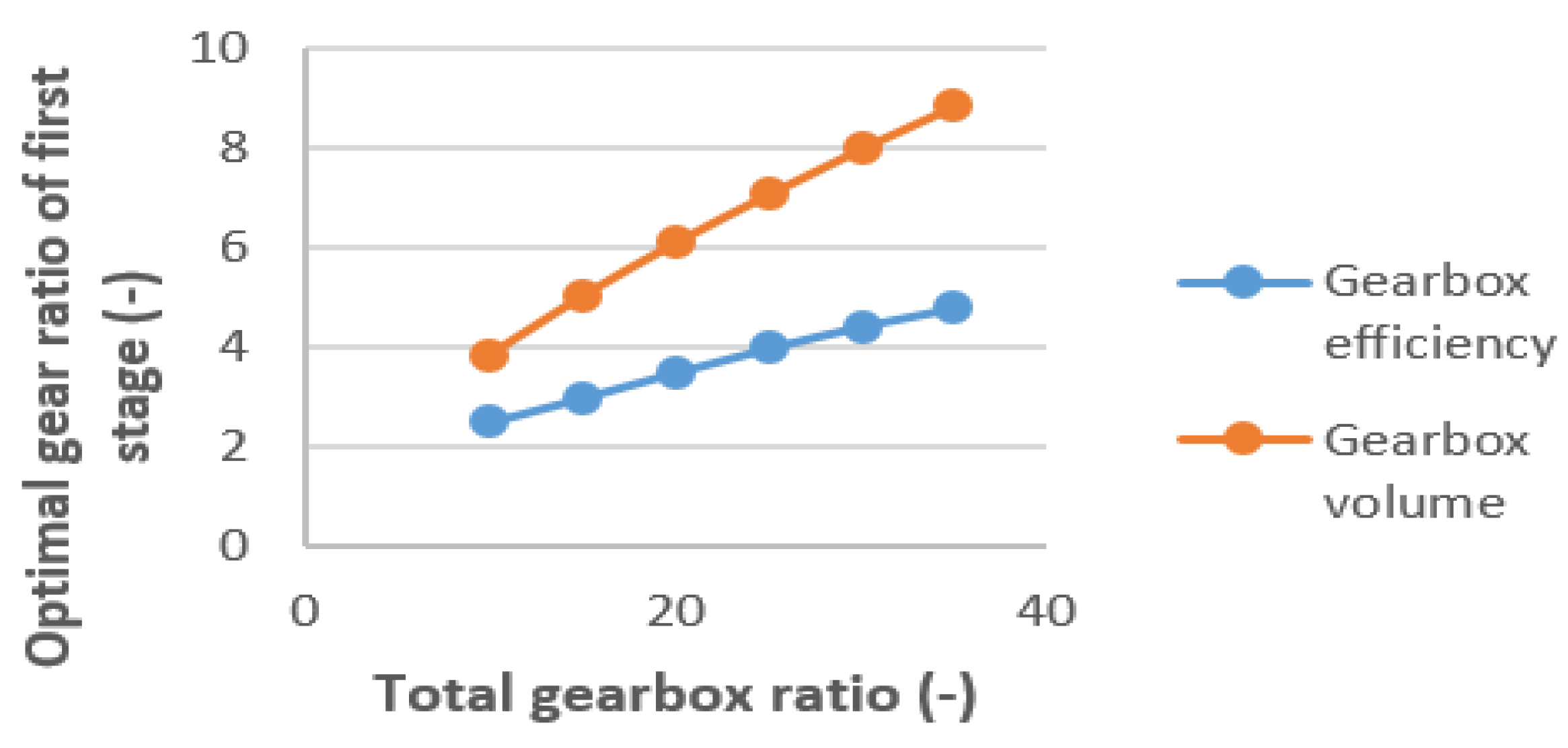
| Objective | Factor | ut | |||||
|---|---|---|---|---|---|---|---|
| 10 | 15 | 20 | 25 | 30 | 35 | ||
| u1 | 3.83 | 5.02 | 6.09 | 7.06 | 7.98 | 8.84 | |
| Vgb | Xba1 | 0.25 | 0.25 | 0.25 | 0.25 | 0.25 | 0.25 |
| Xba2 | 0.4 | 0.4 | 0.4 | 0.4 | 0.4 | 0.4 | |
| u1 | 2.49 | 2.98 | 3.49 | 3.98 | 4.42 | 4.79 | |
| ηgb | Xba1 | 0.25 | 0.25 | 0.25 | 0.25 | 0.25 | 0.25 |
| Xba2 | 0.25 | 0.25 | 0.25 | 0.25 | 0.25 | 0.25 | |
| ut | u1 | |
|---|---|---|
| Lower Limit | Upper Limit | |
| 10 | 2.39 | 2.93 |
| 15 | 3.08 | 5.12 |
| 20 | 3.59 | 6.19 |
| 25 | 4.08 | 7.16 |
| 30 | 4.52 | 8.08 |
| 35 | 4.89 | 8.94 |
| Trial | u1 | Xba1 | Xba2 | Vgb (dm3) | egb (%) |
|---|---|---|---|---|---|
| 1 | 3.61 | 0.25 | 0.25 | 21.05 | 95.906 |
| 2 | 3.61 | 0.25 | 0.2875 | 20.41 | 95.963 |
| 3 | 3.61 | 0.25 | 0.325 | 19.91 | 95.947 |
| 4 | 3.61 | 0.25 | 0.3625 | 19.52 | 95.931 |
| 5 | 3.61 | 0.25 | 0.4 | 19.19 | 95.902 |
| 6 | 3.61 | 0.2875 | 0.25 | 21.35 | 95.407 |
| … | |||||
| 25 | 3.61 | 0.4 | 0.4 | 19.95 | 93.52 |
| 26 | 3.63 | 0.25 | 0.25 | 21.01 | 95.888 |
| 27 | 3.63 | 0.25 | 0.2875 | 20.38 | 95.946 |
| … | |||||
| 51 | 3.65 | 0.25 | 0.25 | 20.98 | 95.852 |
| 52 | 3.65 | 0.25 | 0.2875 | 20.34 | 95.929 |
| 53 | 3.65 | 0.25 | 0.325 | 19.84 | 95.913 |
| … | |||||
| 75 | 3.67 | 0.4 | 0.4 | 19.86 | 93.42 |
| 76 | 3.67 | 0.25 | 0.25 | 20.94 | 95.837 |
| 77 | 3.67 | 0.25 | 0.2875 | 20.31 | 95.911 |
| … | |||||
| 104 | 3.69 | 0.25 | 0.3625 | 19.39 | 95.852 |
| 105 | 3.69 | 0.25 | 0.4 | 19.07 | 95.836 |
| 106 | 3.69 | 0.2875 | 0.25 | 21.21 | 95.306 |
| … | |||||
| 123 | 3.69 | 0.4 | 0.325 | 20.74 | 93.434 |
| 124 | 3.69 | 0.4 | 0.3625 | 20.24 | 93.405 |
| 125 | 3.69 | 0.4 | 0.4 | 19.82 | 93.387 |
| Trial | K− | K+ | f(K−) | f(K+) | f(Ki) | Rank |
|---|---|---|---|---|---|---|
| 1 | 0.0084 | 0.0084 | 0.4990 | 0.5010 | 0.0056 | 87 |
| 2 | 0.0085 | 0.0085 | 0.4990 | 0.5010 | 0.0057 | 58 |
| 3 | 0.0087 | 0.0086 | 0.4990 | 0.5010 | 0.0058 | 30 |
| 4 | 0.0088 | 0.0087 | 0.4990 | 0.5010 | 0.0058 | 15 |
| 5 | 0.0088 | 0.0088 | 0.4990 | 0.5010 | 0.0059 | 5 |
| 6 | 0.0083 | 0.0083 | 0.4990 | 0.5010 | 0.0055 | 101 |
| … | ||||||
| 25 | 0.0085 | 0.0085 | 0.4990 | 0.5010 | 0.0057 | 56 |
| 26 | 0.0084 | 0.0084 | 0.4990 | 0.5010 | 0.0056 | 84 |
| 27 | 0.0085 | 0.0085 | 0.4990 | 0.5010 | 0.0057 | 55 |
| … | ||||||
| 51 | 0.0084 | 0.0084 | 0.4990 | 0.5010 | 0.0056 | 83 |
| 52 | 0.0085 | 0.0085 | 0.4990 | 0.5010 | 0.0057 | 52 |
| 53 | 0.0087 | 0.0086 | 0.4990 | 0.5010 | 0.0058 | 28 |
| … | ||||||
| 75 | 0.0085 | 0.0085 | 0.4990 | 0.5010 | 0.0057 | 49 |
| 76 | 0.0084 | 0.0084 | 0.4990 | 0.5010 | 0.0056 | 82 |
| 77 | 0.0086 | 0.0085 | 0.4990 | 0.5010 | 0.0057 | 50 |
| … | ||||||
| 104 | 0.0088 | 0.0087 | 0.4990 | 0.5010 | 0.0058 | 9 |
| 105 | 0.0088 | 0.0088 | 0.4990 | 0.5010 | 0.0059 | 1 |
| 106 | 0.0083 | 0.0083 | 0.4990 | 0.5010 | 0.0055 | 95 |
| … | ||||||
| 123 | 0.0083 | 0.0083 | 0.4990 | 0.5010 | 0.0055 | 91 |
| 124 | 0.0085 | 0.0084 | 0.4990 | 0.5010 | 0.0056 | 69 |
| 125 | 0.0085 | 0.0085 | 0.4990 | 0.5010 | 0.0057 | 46 |
| No. | ut | |||||
|---|---|---|---|---|---|---|
| 10 | 15 | 20 | 25 | 30 | 35 | |
| u1 | 3.55 | 3.69 | 4.18 | 4.47 | 5.06 | 5.39 |
| Xba1 | 0.25 | 0.25 | 0.25 | 0.25 | 0.25 | 0.25 |
| Xba2 | 0.4 | 0.4 | 0.4 | 0.4 | 0.4 | 0.4 |
Disclaimer/Publisher’s Note: The statements, opinions and data contained in all publications are solely those of the individual author(s) and contributor(s) and not of MDPI and/or the editor(s). MDPI and/or the editor(s) disclaim responsibility for any injury to people or property resulting from any ideas, methods, instructions or products referred to in the content. |
© 2024 by the authors. Licensee MDPI, Basel, Switzerland. This article is an open access article distributed under the terms and conditions of the Creative Commons Attribution (CC BY) license (https://creativecommons.org/licenses/by/4.0/).
Share and Cite
Dinh, V.-T.; Tran, H.-D.; Tran, Q.-H.; Vu, D.-B.; Vu, D.; Vu, N.-P.; Nguyen, T.-T. Multi-Objective Optimization of a Two-Stage Helical Gearbox Using MARCOS Method. Designs 2024, 8, 53. https://doi.org/10.3390/designs8030053
Dinh V-T, Tran H-D, Tran Q-H, Vu D-B, Vu D, Vu N-P, Nguyen T-T. Multi-Objective Optimization of a Two-Stage Helical Gearbox Using MARCOS Method. Designs. 2024; 8(3):53. https://doi.org/10.3390/designs8030053
Chicago/Turabian StyleDinh, Van-Thanh, Huu-Danh Tran, Quoc-Hung Tran, Duc-Binh Vu, Duong Vu, Ngoc-Pi Vu, and Thanh-Tu Nguyen. 2024. "Multi-Objective Optimization of a Two-Stage Helical Gearbox Using MARCOS Method" Designs 8, no. 3: 53. https://doi.org/10.3390/designs8030053
APA StyleDinh, V.-T., Tran, H.-D., Tran, Q.-H., Vu, D.-B., Vu, D., Vu, N.-P., & Nguyen, T.-T. (2024). Multi-Objective Optimization of a Two-Stage Helical Gearbox Using MARCOS Method. Designs, 8(3), 53. https://doi.org/10.3390/designs8030053