


Experimental Fitting of Efficiency Hill Chart for Kaplan Hydraulic Turbine


Abstract
:1. Introduction: The Characteristic Curves of Hydraulic Turbines
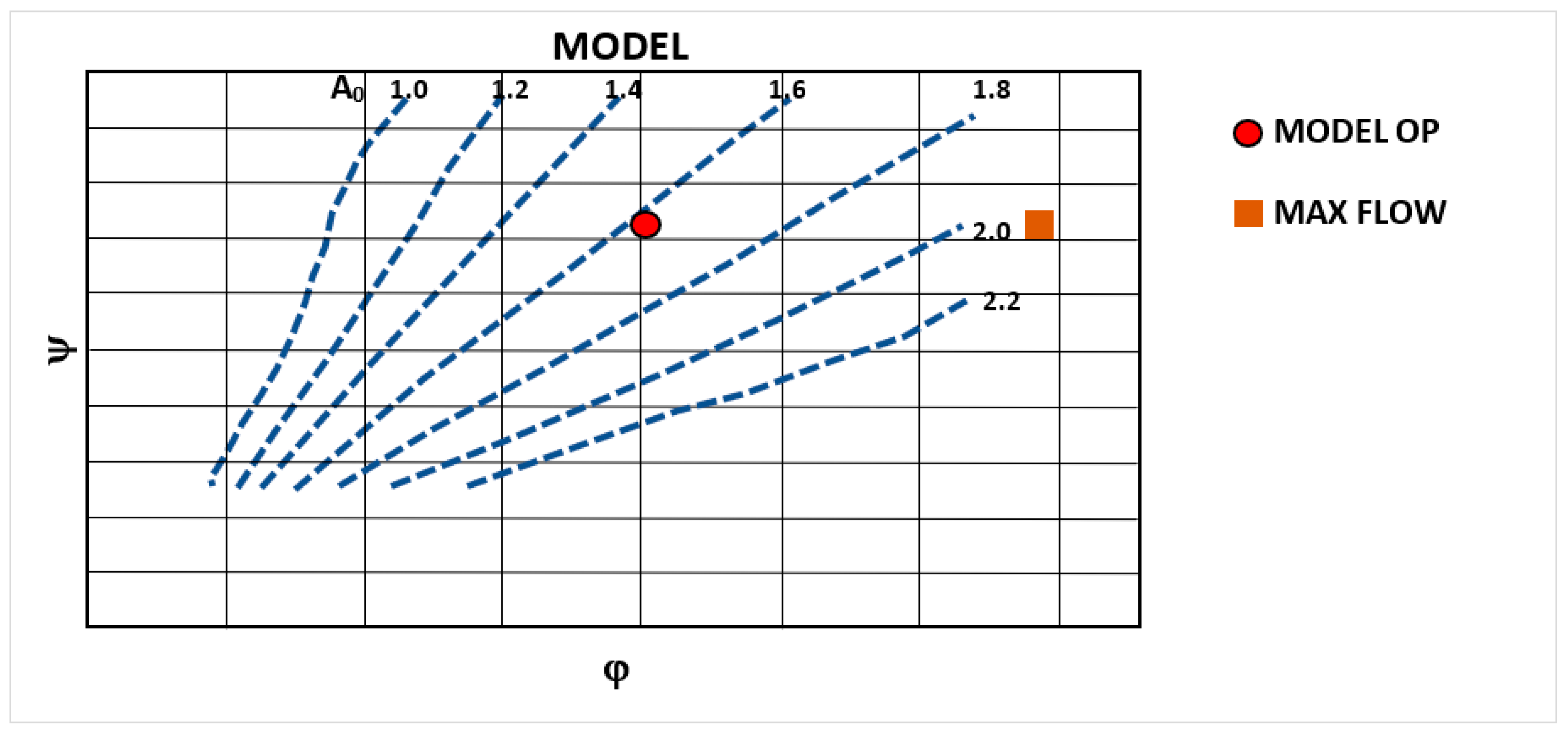
2. The Operational Parameters
- Specific speed;
- Flow coefficient ;
- Load coefficient .
- -
- Model-specific flow rate: ;
- -
- Model-specific speed: .
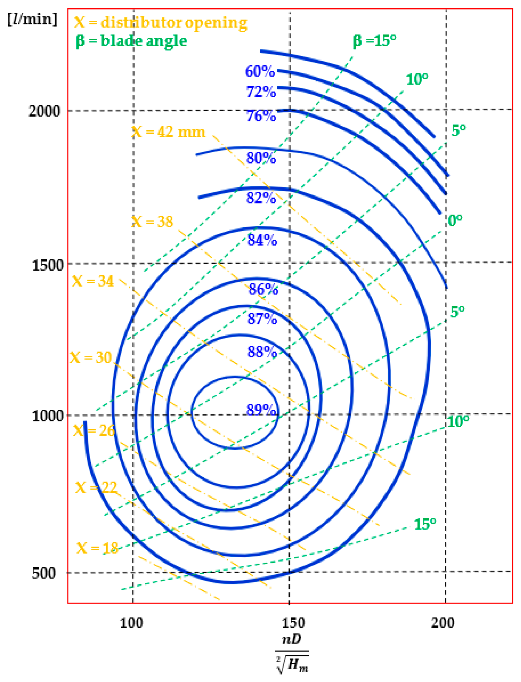
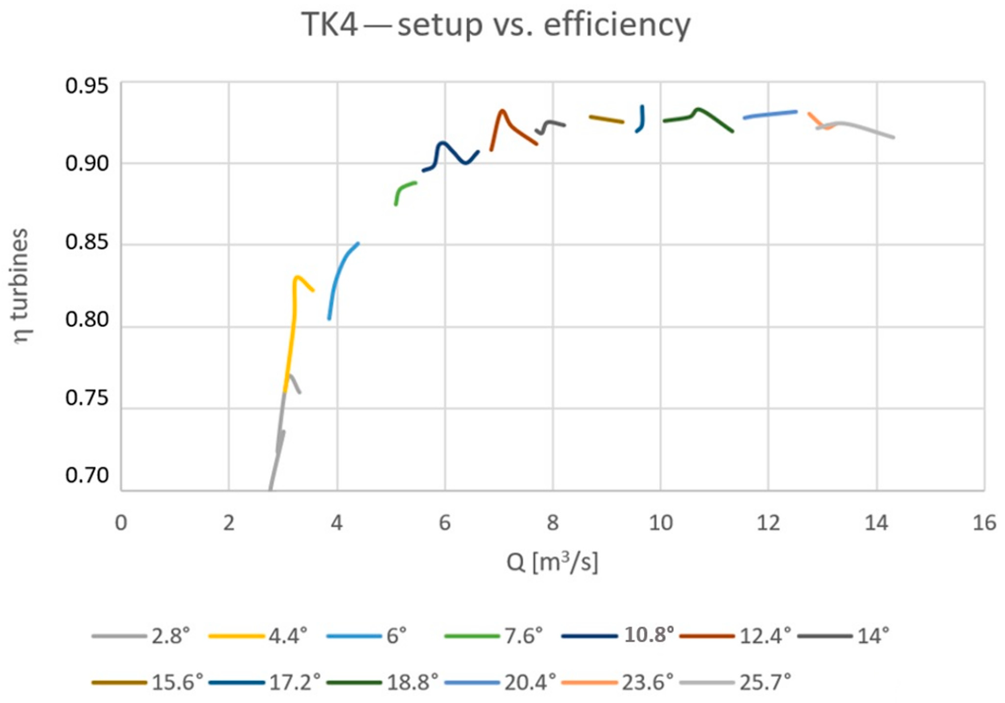
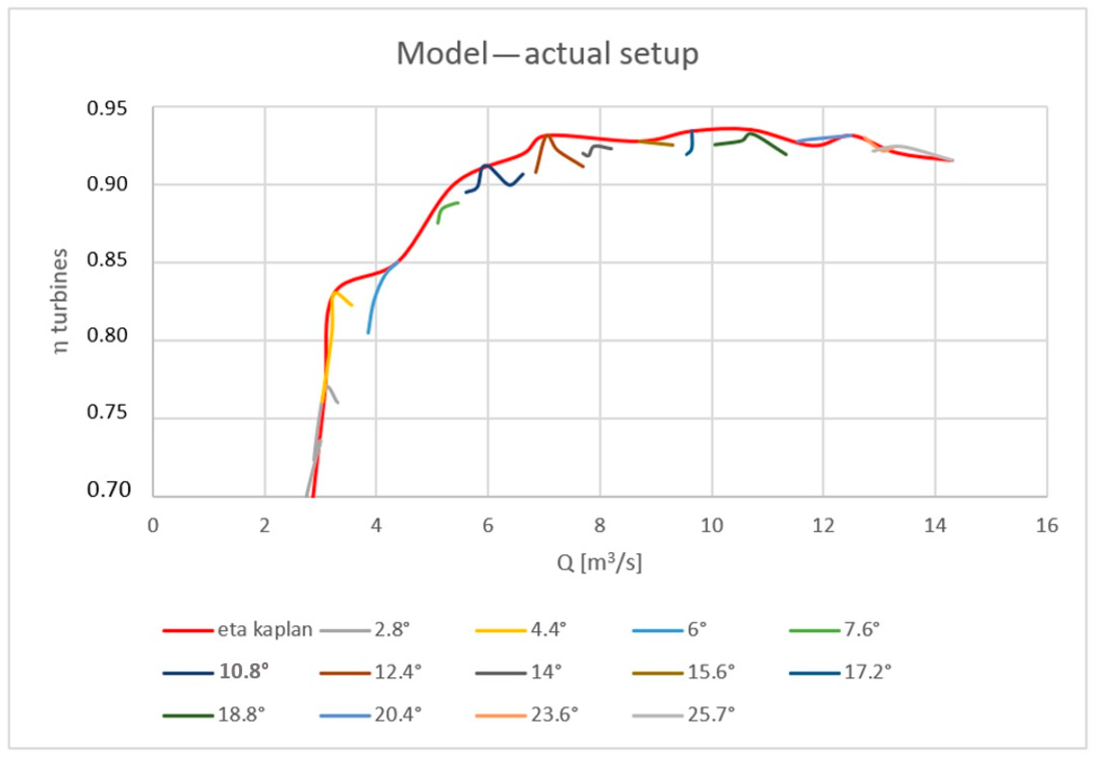
3. The Prototype Tests
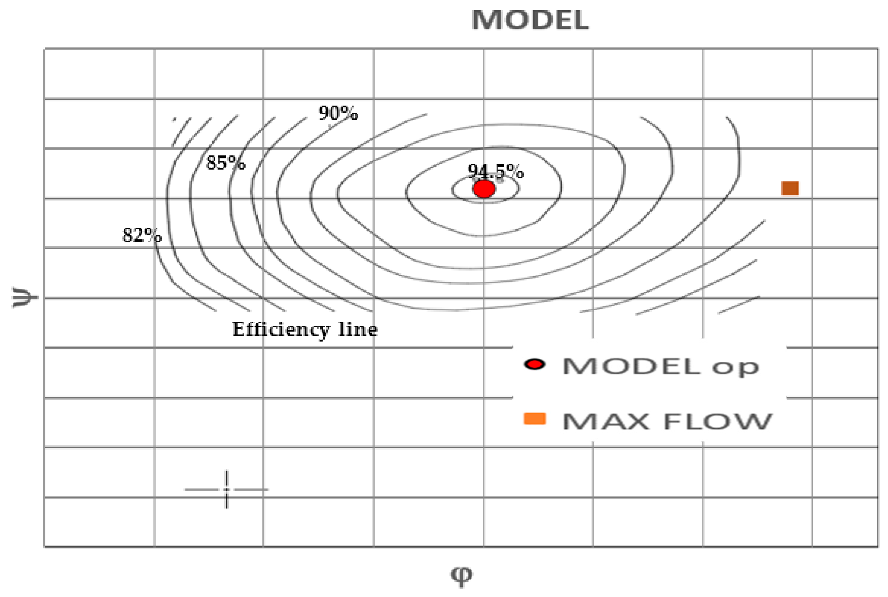
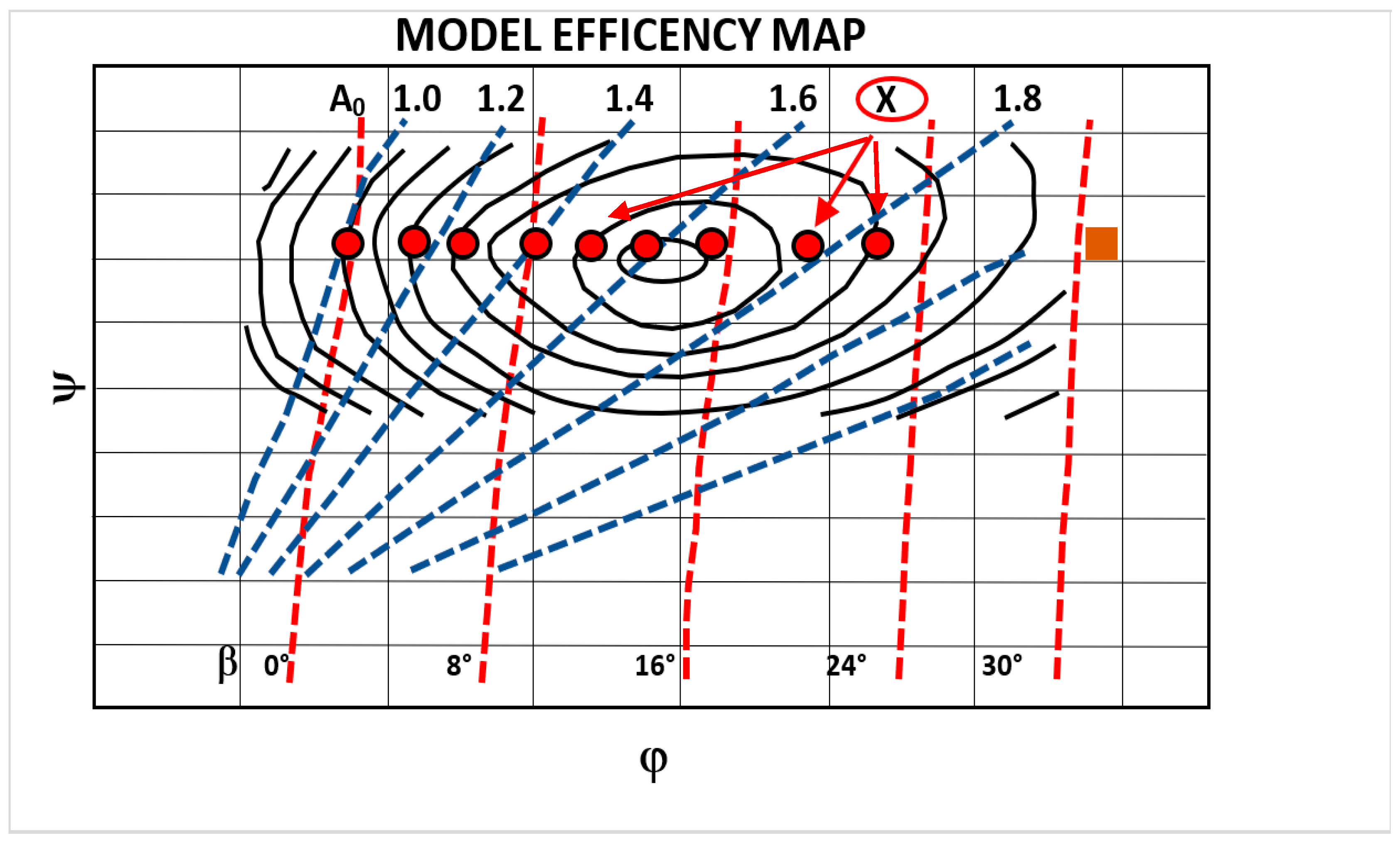
Determination of Efficiency Contour Map
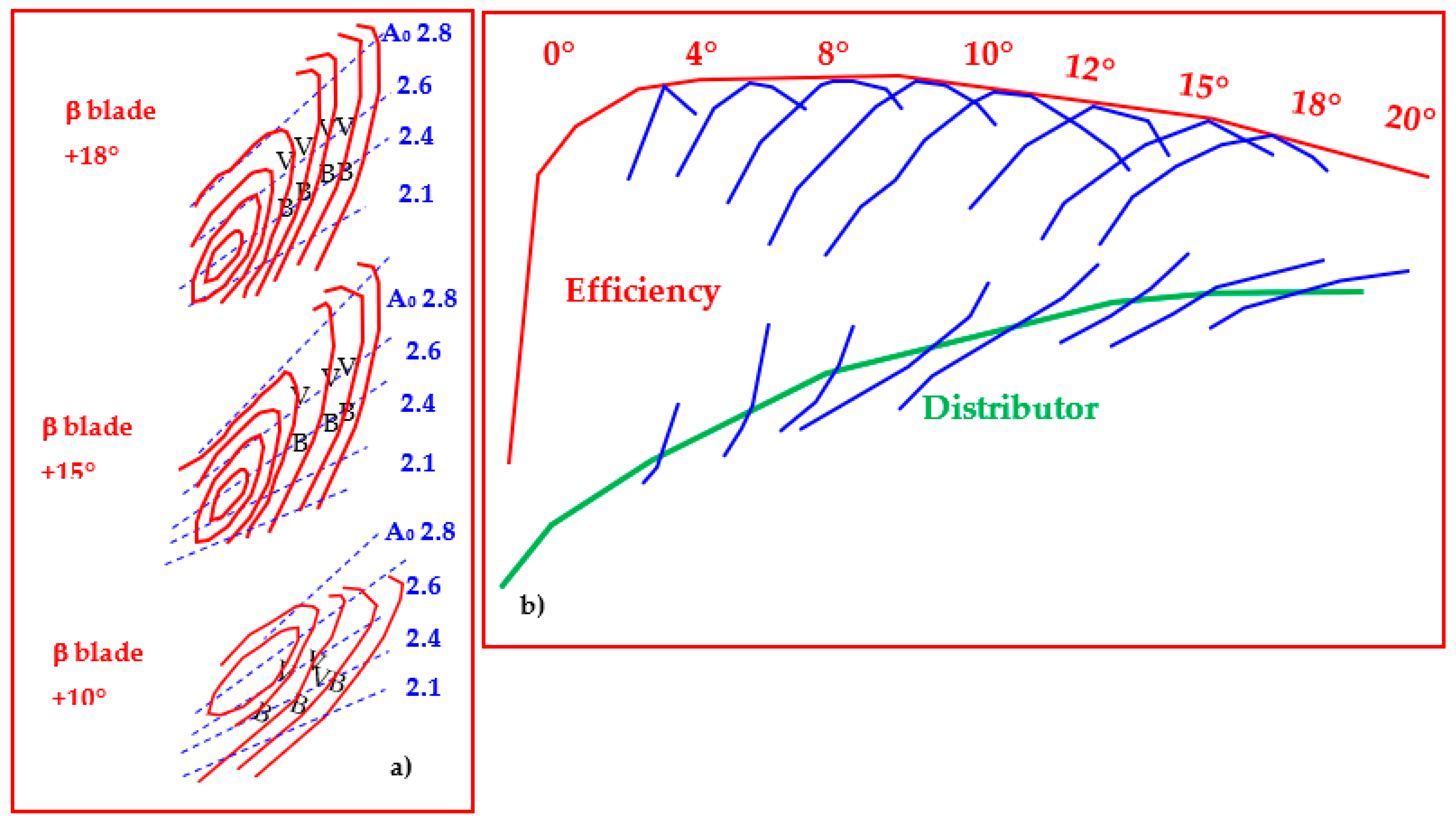
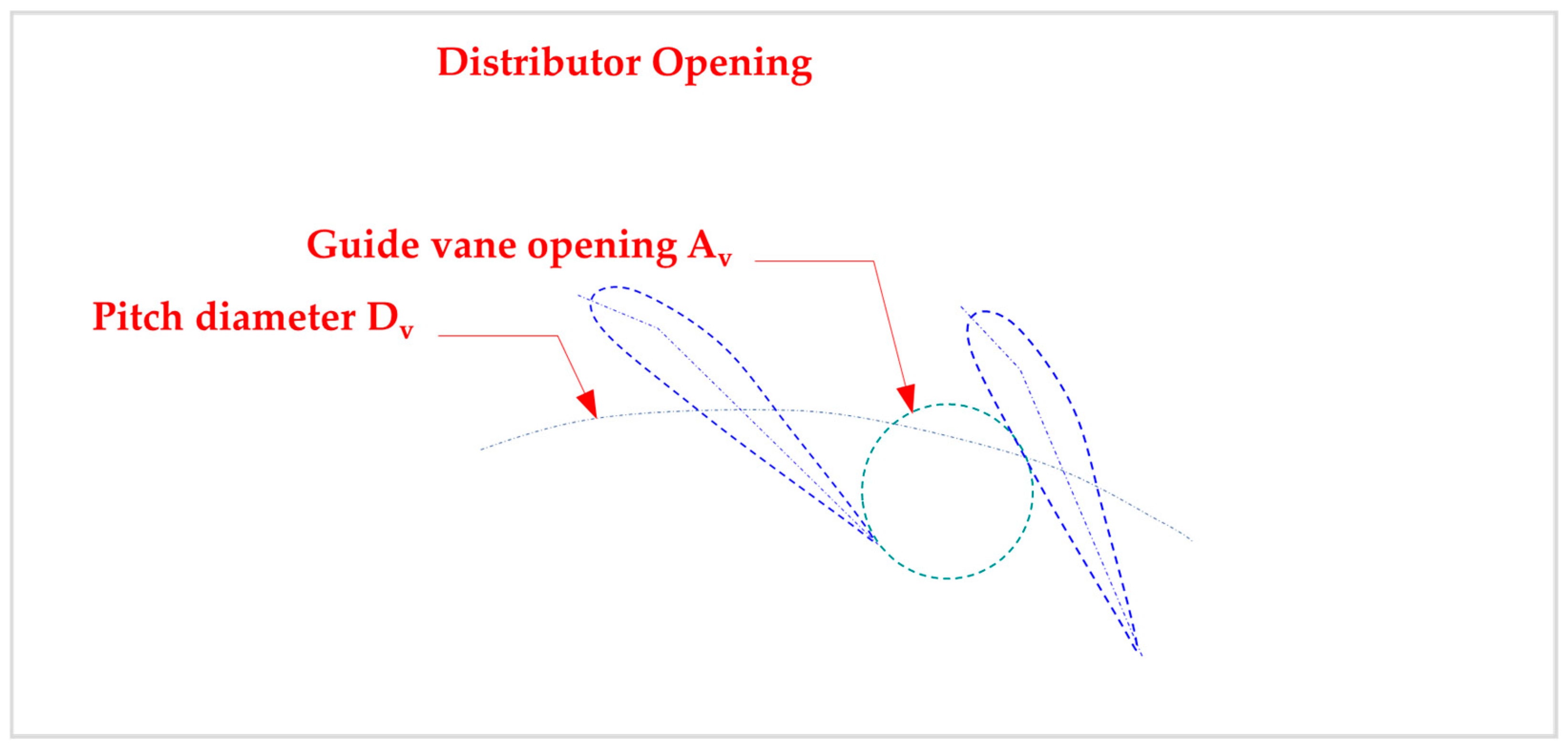
4. Stator/Rotor Setup
- -
- = diameter of the passing sphere [m];
- -
- = number of distributor blades;
- -
- = pitch diameter [m];
- -
- = specific opening degree [m].
5. Conclusions
Author Contributions
Funding
Data Availability Statement
Conflicts of Interest
References
- Balje, O.E. Turbomachines: A Guide to Design, Selection and Theory; John Wiley Sons Inc.: Hoboken, NJ, USA, 1981. [Google Scholar]
- Dixon, S.L.; Hall, C. Fluid Mechanics and Thermodynamics of Turbomachinery. Butterworth-Heinemann 2013, 7th ed.; Butterworth-Heinemann: Oxford, UK, 2013. [Google Scholar]
- Shepherd, D.G. Principles of Turbomachinery; MacMillan: New York, NY, USA, 1971. [Google Scholar]
- Krivchenko, G.I. Hydraulic Machines—Turbines and Pumps, 2nd ed.; Lewis Publishers: Boca Raton, FL, USA; IEC: Geneva, Switzerland, 1994. [Google Scholar]
- IEC 60041; Field Acceptance Tests to Determine the Hydraulic Performance of Hydraulic Turbines, Storage Pumps and Pump-Turbines. IEC: Geneva, Switzerland, 1991. Available online: https://www.saiglobal.com/pdftemp/previews/osh/iec/iec60000/60000/iec60041%7Bed3.0%7Den_d.img.pdf (accessed on 4 November 2023).
- Vu, T.C.; Koller, M.; Gauthier, M.; Deschênes, C. Flow simulation and efficiency hill chart prediction for a Propeller turbine. In Proceedings of the 25th IAHR Symposium on Hydraulic Machinery and Systems. IOP Conf. Ser. Earth Environ. Sci. 2010, 12, 012040. [Google Scholar] [CrossRef]
- Iliev, I.; Trivedi, C.; Dahlhaug, O.G. Simplified hydrodynamic analysis on the general shape of the hill charts of Francis turbines using shroud-streamline modeling. Current Research in Hydraulic Turbines (CRHT) VIII. IOP J. Phys. Conf. Ser. 2018, 1042, 012003. [Google Scholar] [CrossRef]
- Guo, P.; Wang, Z.; Sun, L.; Luo, X. Characteristic analysis of the efficiency hill chart of Francis turbine for different water heads. Adv. Mech. Eng. 2017, 9, 1–8. [Google Scholar] [CrossRef]
- IEC 995; Determination of the Prototype Performance from Model Acceptance Tests of Hydraulic Machines. IEC: Geneva, Switzerland, 1991.
- IEC 193; Hydraulic Turbines, Storage Pumps and Pump-Turbines—Model Acceptance Tests. IEC: Geneva, Switzerland, 2019.
- IEC 60609; Hydraulic Turbines, Storage Pumps and Pump-Turbines—Cavitation Pitting Evaluation—Part 1: Evaluation in Reaction Turbines, Storage Pumps and Pump-Turbines. IEC: Geneva, Switzerland, 2004.
- IEC 60609; Hydraulic Turbines, Storage Pumps and Pump-Turbines—Cavitation Pitting Evaluation—Part 2: Evaluation in Pelton Turbines. IEC: Geneva, Switzerland, 2004.
- Simão, M.; Ramos, H.M. Micro Axial Turbine Hill Charts: Affinity Laws, Experiments and CFD Simulations for Different Diameters. Energies 2019, 12, 2908. [Google Scholar] [CrossRef]
- Borghetti, A.; Di Silvestro, M.; Naldi, G.; Paolone, M.; Alberti, M. Maximum Efficiency Point Tracking for Adjustable-Speed Small Hydro Power Plant. In Proceedings of the 16th PSCC, Glasgow, Scotland, 14–18 July 2008. [Google Scholar]
- Cinquepalmi, F.; Piras, G. Earth Observation Technologies for Mitigating Urban Climate Changes. In Technological Imagination in the Green and Digital Transition; CONF.ITECH 2022. The Urban Book Series; Springer: Cham, Switzerland, 2023. [Google Scholar] [CrossRef]
- Capata, R.; Piras, G. Condenser Design for On-Board ORC Recovery System. Appl. Sci. 2021, 11, 6356. [Google Scholar] [CrossRef]
- Piras, G.; Muzi, F. Energy Transition: Semi-Automatic BIM Tool Approach for Elevating Sustainability in the Maputo Natural History Museum. Energies 2024, 17, 775. [Google Scholar] [CrossRef]


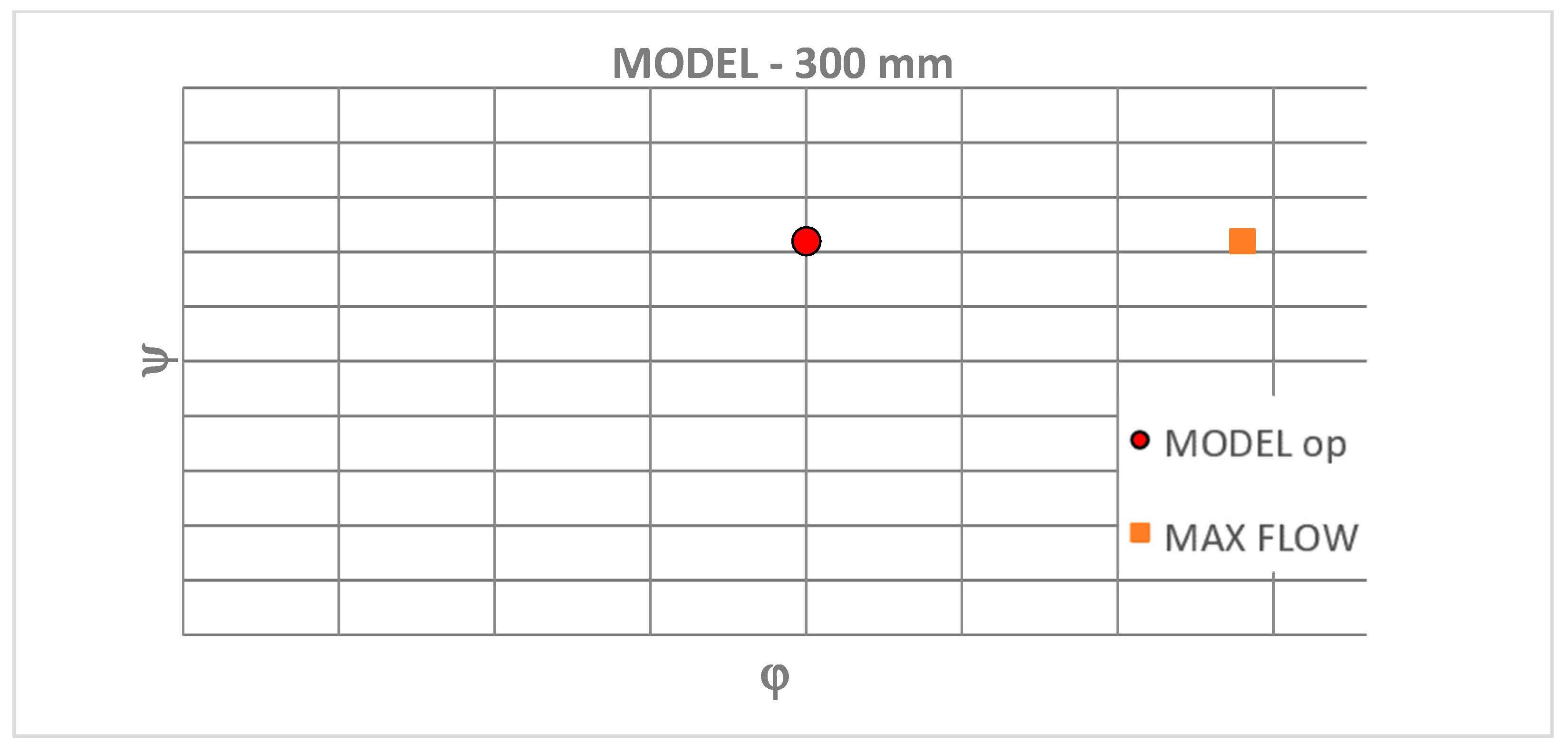
| Model Type | Turbine Characteristics | ||
|---|---|---|---|
| Optimal flow coefficient | ϕopt | 0.20 | [-] |
| Optimal load coefficient | ψopt | 0.36 | [-] |
| Model optimum efficiency | ηopt | 0.915 | [-] |
| Specific speed | Ns | 554 | [-] |
| Flow coefficient max at ψopt | ϕopt | 0.34 | [-] |
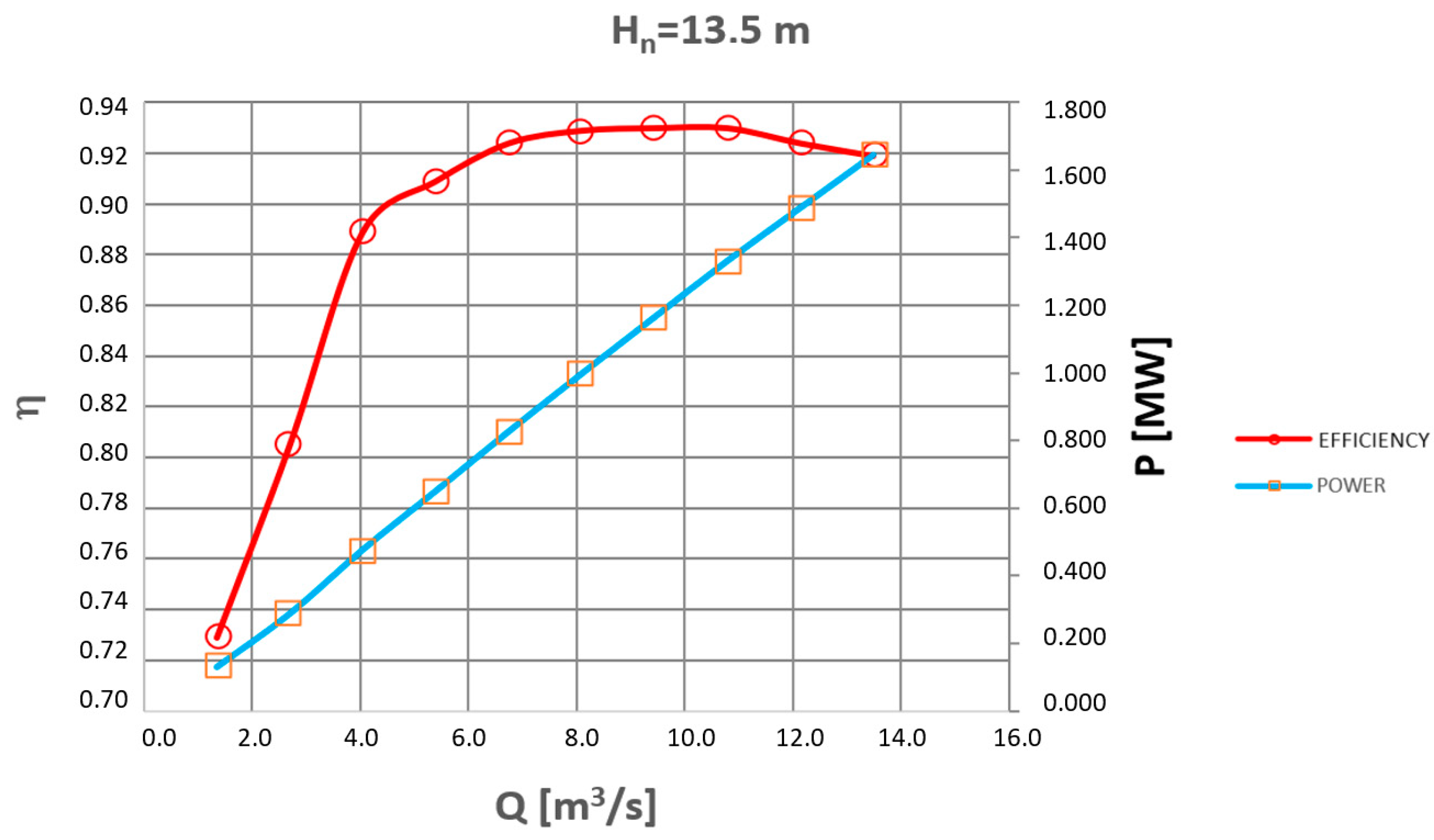
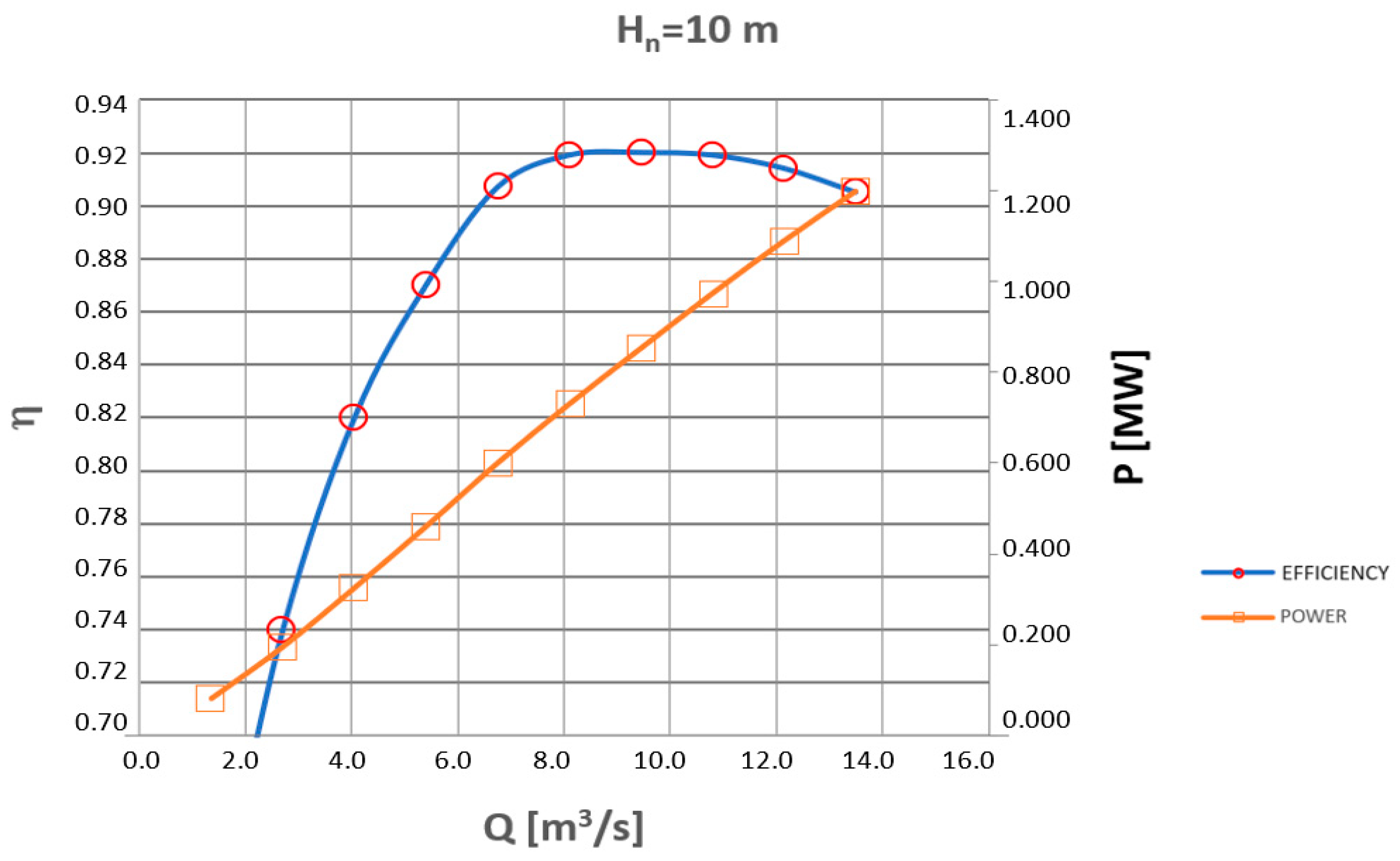
| Hn = 13.5 m | Hn = 10 m | ||||||||
|---|---|---|---|---|---|---|---|---|---|
| Q | Hn | ψ | φ | η | Q | Hn | ψ | φ | η |
| [m3/s] | [m] | [-] | [-] | [%] | [m3/s] | [m] | [-] | [-] | [%] |
| 1.35 | 13.5 | 0.387 | 0.029 | 72.9 | 1.35 | 10 | 0.287 | 0.029 | 62 |
| 2.7 | 13.5 | 0.387 | 0.058 | 80.5 | 2.7 | 10 | 0.287 | 0.058 | 74 |
| 4.05 | 13.5 | 0.387 | 0.087 | 88.9 | 4.05 | 10 | 0.287 | 0.088 | 82 |
| 5.4 | 13.5 | 0.387 | 0.116 | 90.9 | 5.4 | 10 | 0.287 | 0.117 | 87 |
| 6.75 | 13.5 | 0.387 | 0.146 | 92.4 | 6.75 | 10 | 0.287 | 0.146 | 90.7 |
| 8.1 | 13.5 | 0.387 | 0.175 | 92.9 | 8.1 | 10 | 0.287 | 0.175 | 91.9 |
| 9.45 | 13.5 | 0.387 | 0.204 | 93 | 9.45 | 10 | 0.287 | 0.204 | 92 |
| 10.8 | 13.5 | 0.387 | 0.233 | 93 | 10.8 | 10 | 0.287 | 0.234 | 91.9 |
| 12.15 | 13.5 | 0.387 | 0.262 | 92.4 | 12.15 | 10 | 0.287 | 0.263 | 91.4 |
| 13.5 | 13.5 | 0.387 | 0.292 | 91.9 | 13.5 | 10 | 0.287 | 0.292 | 90.5 |
| Parameter | Turbomachinery | |||
|---|---|---|---|---|
| Radial (Francis) | Diagonal (Mixed Flow) | Axial (Kaplan, Bulb) | Impulse (Pelton) | |
| Reynolds number Re | 4 × 10⁶ | 4 × 10⁶ | 4 × 10⁶ | 2 × 10⁶ |
| Specific hydraulic energy E [J/kg] | 100 | 50 | 30 | 500 |
| Reference diameter D [m] | 0.25 | 0.3 | 0.3 | ----- |
| Bucket width [m] | ----- | ----- | ----- | 0.08 |
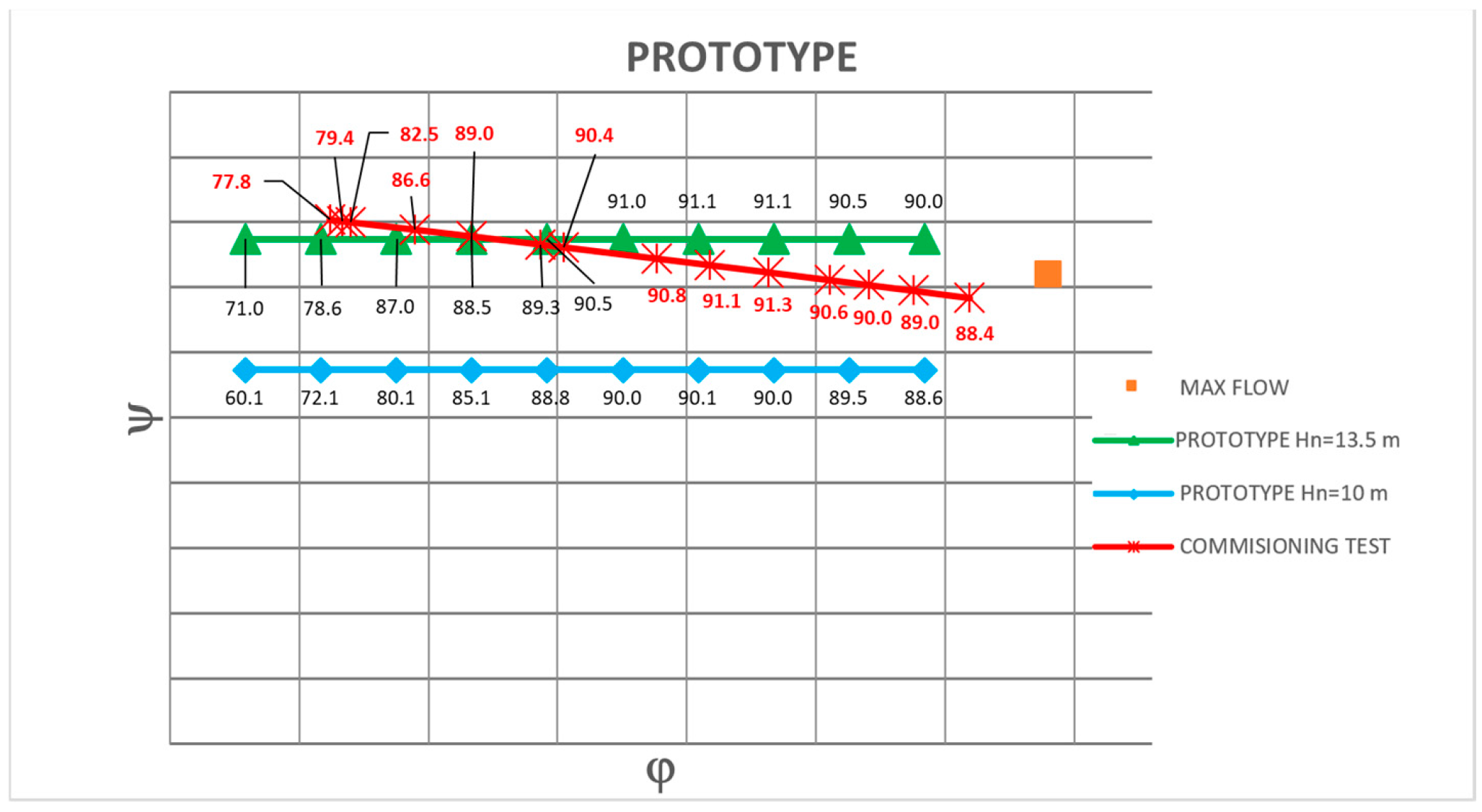
| Runner | Distributor | Hn | P | ψ | φ | ηprototype | ηmodel | |
|---|---|---|---|---|---|---|---|---|
| [%] | [%] | [m3/s] | [m] | [kW] | [-] | [-] | [%] | [%] |
| 5.5 | 45 | 2.86 | 11.35 | 260 | 0.326 | 0.062 | 79.6 | 77.8 |
| 8.7 | 47 | 3.08 | 11.19 | 285 | 0.321 | 0.067 | 81.3 | 79.4 |
| 11 | 48 | 3.23 | 11.05 | 310 | 0.317 | 0.070 | 84.4 | 82.5 |
| 20 | 50 | 4.38 | 10.87 | 470 | 0.312 | 0.095 | 88.4 | 86.6 |
| 27 | 58 | 5.4 | 10.71 | 590 | 0.307 | 0.117 | 90.4 | 88.5 |
| 35 | 65 | 6.62 | 10.52 | 725 | 0.302 | 0.143 | 91.2 | 89.3 |
| 40 | 67 | 7.04 | 10.42 | 780 | 0.299 | 0.152 | 92.2 | 90.4 |
| 50 | 75 | 8.7 | 10.19 | 955 | 0.292 | 0.188 | 92.7 | 90.8 |
| 56 | 80 | 9.65 | 10.03 | 1050 | 0.288 | 0.209 | 93.0 | 91.1 |
| 65 | 82 | 10.7 | 9.83 | 1150 | 0.282 | 0.232 | 93.1 | 91.3 |
| 72 | 85 | 11.8 | 9.62 | 1240 | 0.276 | 0.255 | 92.5 | 90.6 |
| 78 | 87 | 12.5 | 9.44 | 1290 | 0.271 | 0.270 | 91.9 | 90.0 |
| 80 | 90 | 13.3 | 9.39 | 1340 | 0.269 | 0.288 | 90.8 | 89.0 |
| 90 | 97 | 14.3 | 9 | 1410 | 0.258 | 0.309 | 90.3 | 88.4 |
| Plant | Solution | D | n | H | Q | φ | ψ |
|---|---|---|---|---|---|---|---|
| [mm] | [rpm] | [m] | [m3/s] | [-] | [-] | ||
| 1 | 1 | 1500 | 333 | 333 | 11.05 | 0.317 | 0.292 |
| 2 | 2 | 950 | 300 | 300 | 4.6 | 0.405 | 0.284 |
| 3 | 3 | 1500 | 250 | 250 | 6.7 | 0.341 | 0.317 |
| 4 | 4 | 700 | 750 | 750 | 11.9 | 0.309 | 0.227 |
| 5 | 5 | 900 | 428 | 428 | 6.9 | 0.333 | 0.281 |
| 6 | 975 | 375 | 375 | 6.9 | 0.369 | 0.252 | |
| 7 | 850 | 428 | 428 | 6.9 | 0.373 | 0.278 | |
| 6 | 8 | 680 | 500 | 500 | 6.3 | 0.390 | 0.309 |
| 9 | 700 | 500 | 500 | 6.3 | 0.368 | 0.284 | |
| 7 | 10 | 1150 | 375 | 375 | 9.7 | 0.373 | 0.298 |
| 8 | 11 | 3500 | 75 | 75 | 3.7 | 0.384 | 0.302 |
| 9 | 12 | 1400 | 175 | 175 | 3.4 | 0.405 | 0.304 |
| 10 | 13 | 800 | 600 | 600 | 12.2 | 0.379 | 0.237 |
| 11 | 14 | 1800 | 231 | 231 | 7.5 | 0.310 | 0.271 |
| 12 | 15 | 1000 | 500 | 500 | 10.8 | 0.309 | 0.292 |
| 13 | 16 | 1450 | 250 | 250 | 6.2 | 0.338 | 0.319 |
| 14 | 17 | 1150 | 375 | 375 | 7.7 | 0.296 | 0.277 |
| 15 | 18 | 1600 | 250 | 250 | 6.6 | 0.295 | 0.285 |
| 16 | 19 | 1900 | 200 | 200 | 6.15 | 0.305 | 0.319 |
| 17 | 20 | 2100 | 187 | 187 | 5.9 | 0.274 | 0.329 |
| 18 | 21 | 2560 | 167 | 167 | 7 | 0.274 | 0.295 |
| 19 | 22 | 2950 | 136 | 136 | 7.8 | 0.347 | 0.258 |
| 23 | 2950 | 136 | 136 | 7.7 | 0.342 | 0.258 | |
| 24 | 2950 | 136 | 136 | 9.2 | 0.409 | 0.258 | |
| 25 | 2950 | 136 | 136 | 7.4 | 0.329 | 0.258 | |
| 26 | 2950 | 136 | 136 | 7.3 | 0.325 | 0.258 | |
| 27 | 2950 | 136 | 136 | 9.1 | 0.405 | 0.258 | |
| 28 | 2600 | 200 | 220 | 17.5 | 0.383 | 0.233 | |
| 20 | 29 | 950 | 375 | 375 | 6 | 0.338 | 0.310 |
| 21 | 30 | 740 | 375 | 375 | 4.25 | 0.395 | 0.280 |
| 22 | 31 | 920 | 333 | 333 | 4.6 | 0.351 | 0.281 |
| 23 | 32 | 3500 | 75 | 82 | 4.2 | 0.365 | 0.277 |
| 24 | 33 | 1250 | 428 | 428 | 14.1 | 0.353 | 0.291 |
| 34 | 1250 | 428 | 428 | 15 | 0.375 | 0.291 | |
| 35 | 1250 | 428 | 428 | 16.12 | 0.403 | 0.291 | |
| 25 | 36 | 540 | 600 | 600 | 5.5 | 0.375 | 0.257 |
| 37 | 540 | 600 | 600 | 5.5 | 0.375 | 0.257 | |
| 26 | 38 | 743 | 300 | 300 | 2.65 | 0.382 | 0.267 |
| 27 | 39 | 2747 | 187.5 | 187.5 | 12.5 | 0.337 | 0.288 |
| 28 | 40 | 1350 | 300 | 300 | 7.5 | 0.327 | 0.297 |
| 41 | 1550 | 250 | 250 | 7.5 | 0.357 | 0.235 | |
| 29 | 42 | 2550 | 120 | 140 | 5.9 | 0.331 | 0.241 |
| 30 | 43 | 670 | 500 | 500 | 5.3 | 0.338 | 0.323 |
| 31 | 44 | 550 | 750 | 750 | 9 | 0.379 | 0.292 |
| 32 | 45 | 850 | 500 | 500 | 10.3 | 0.408 | 0.277 |
| 33 | 46 | 5000 | 100 | 100 | 10.3 | 0.295 | 0.324 |
Disclaimer/Publisher’s Note: The statements, opinions and data contained in all publications are solely those of the individual author(s) and contributor(s) and not of MDPI and/or the editor(s). MDPI and/or the editor(s) disclaim responsibility for any injury to people or property resulting from any ideas, methods, instructions or products referred to in the content. |
© 2024 by the authors. Licensee MDPI, Basel, Switzerland. This article is an open access article distributed under the terms and conditions of the Creative Commons Attribution (CC BY) license (https://creativecommons.org/licenses/by/4.0/).
Share and Cite
Capata, R.; Calabria, A.; Baralis, G.M.; Piras, G. Experimental Fitting of Efficiency Hill Chart for Kaplan Hydraulic Turbine. Designs 2024, 8, 80. https://doi.org/10.3390/designs8040080
Capata R, Calabria A, Baralis GM, Piras G. Experimental Fitting of Efficiency Hill Chart for Kaplan Hydraulic Turbine. Designs. 2024; 8(4):80. https://doi.org/10.3390/designs8040080
Chicago/Turabian StyleCapata, Roberto, Alfonso Calabria, Gian Marco Baralis, and Giuseppe Piras. 2024. "Experimental Fitting of Efficiency Hill Chart for Kaplan Hydraulic Turbine" Designs 8, no. 4: 80. https://doi.org/10.3390/designs8040080
APA StyleCapata, R., Calabria, A., Baralis, G. M., & Piras, G. (2024). Experimental Fitting of Efficiency Hill Chart for Kaplan Hydraulic Turbine. Designs, 8(4), 80. https://doi.org/10.3390/designs8040080