Abstract
The monolithic composite action of structures relies on the interface bond strength between concrete and the repair material. This study uses explainable deep learning techniques to evaluate the ultimate strength capacity (Us) of U-shaped normal concrete (NC) strengthened with polyurethane grouting (PUG) materials. Machine learning algorithms (ML) such as Long Short-Term Memory (LSTM), Random Forest (RF), and Wide Neural Network (WNN) models were developed to estimate Us by considering five input parameters: the initial crack strength (Cs), thickness of the grouting materials (T), mid-span deflection (λ), and peak applied load (P). The results indicated that LSTM models, particularly LSTM-M2 and LSTM-M3, demonstrated superior predictive accuracy and consistency in both the calibration and verification phases, as evidenced by high Pearson’s correlation coefficients (PCC = 0.9156 for LSTM-M2) and Willmott indices (WI = 0.7713 for LSTM-M2), and low error metrics (MSE = 0.0017, RMSE = 0.0418). The SHAP (SHapley Additive exPlanations) analysis showed that the thickness of the grouting materials and maximum load were the most significant parameters affecting the ultimate capacity of the composite U-shaped specimen. The RF model showed moderate improvements, with RF-M3 performing better than RF-M1 and RF-M2. The WNN models displayed varied performance, with WNN-M2 performing poorly due to significant scatter and deviation. The findings highlight the potential of LSTM models for the accurate and reliable prediction of the ultimate strength of composite U-shaped specimens.
1. Introduction
Concrete is the most commonly used construction material. However, it has an inherent nature, including brittleness, tensile strength, low ductility, flexural strength, and strain rate sensitivity, and these properties are regarded as deficiencies in concrete structural applications [1,2,3] Polymer materials, including polyethylene, epoxy resins, polyurethane, polystyrene, etc., have been added to concrete to improve its certain properties [4,5,6,7], retrofitting the concrete structure [8] as recycled aggregates [9]. They reduce the brittleness of cement-based materials, have anti-crack properties, and reduce porosity and shrinkage properties [7,10]. Building industries have acknowledged the concrete impact strength as one of its essential properties [11], because concrete buildings are often exposed to impact force during their lifespan. The impact stress exposed to structures includes the effect of water on hydraulic structures [12], projectile masses [13,14,15], and collisions of vehicles with bridge columns [14]. Furthermore, the short-term dynamic stress exerted under the impact force causes concrete to experience exceptional stresses. Consequently, these loadings put the concrete under stress, necessitating a higher microstructure and coating to effectively withstand impact loads. The ability of concrete to absorb force and operate better dynamically is known as impact strength [14,16]. However, developing advanced models that combine the capability of different ML approaches could offer enhanced performance and reliability of the structures, and exploring the potential of transfer learning in this domain may also prove beneficial, allowing models trained on one dataset to be effectively applied to another, thereby reducing the need for extensive experimental programs.
Over the decades, ML techniques have proven promising in modeling construction materials [17,18,19,20,21]. These techniques can determine the relationship between modeling features without prior information, prevailing physical or mathematical theories. Thus, several ML methods have been developed to estimate the bond strength of composite materials [22,23]. Liu et al. [24] established interpretable ML algorithms for estimating the bond behavior between the concrete substrate and ultra-high performance concrete. The authors utilized a dataset of 95 specimens tested under the slant shear test. The result indicated that the models performance surpassed the empirical model established by AASHTO LRFD 2014 and Eurocode 2. Wakjira et al. [22] predicted and developed software for evaluating the bond strength of concrete substrates with corroded rebars. You et al. [25] applied hybrid ML techniques to estimate the ultimate interface bond strength between UHPC and steel bars. The result showed that the proportion of embedded depth to diameter significantly influenced the bond properties. Maj and Czarnecki [26] performed a comparative study to choose ML models to predict the interfacial bond properties of concrete. The bond strength of fiber–concrete subjected to several conditions was predicted using an ML-based graphical interface model [27]. Li et al. [28] trained a database of 335 specimens to quantify the relationships between the reinforcement, concrete, corrosion factors, and bond behavior. Similarly, a robust hybrid optimized XGBoost showed promising results in estimating the compressive strength of sleeve grouting materials in concrete structures [29]. The effect of admixtures on ultra-high performance concrete was evaluated using an ML model [30].
Therefore, upon a review of past studies of ML algorithms, it can be noted that ML algorithms have the capability of handling many parameters, including linear and nonlinear features [31]. For this reason, the ML model was employed in this study to evaluate the ultimate capacity of the composite concrete, which can reflect the interfacial bond strength between the NC substrate with grouting materials under impact load. To fill this gap, this study aims to predict the ultimate capacity of composite U-shaped NC-PUG under repeated drop-weight impact loads by employing explainable deep learning algorithms, specifically involving the static and impact properties of composite U-shaped specimens subjected to splitting tensile, mechanical strength, and repeated impact tests. The advanced deep learning models, including Long Short-Term Memory, Random Forest, and a novel Wide Neural Network, were employed to train the dataset obtained from the experimental program. The modeling work involves the combination of different input features for developing models (M1, M2, and M3). Furthermore, SHapley Additive exPlanationss (SHAP) explainable ML techniques provide valuable insights into the factors influencing the model predictions. The novelty of this research lies in its comprehensive approach to evaluating the ultimate strength capacity under repeated impact loading conditions, which is less explored in the existing literature, and in integrating explainable AI (XAI) to enhance the interpretability and reliability of the predictive models. This study advances machine learning applications in forecasting and explaining material performance while offering a deeper understanding of the bond behavior of composite structures responsible for monolithic behavior.
2. Description of the Developed Database
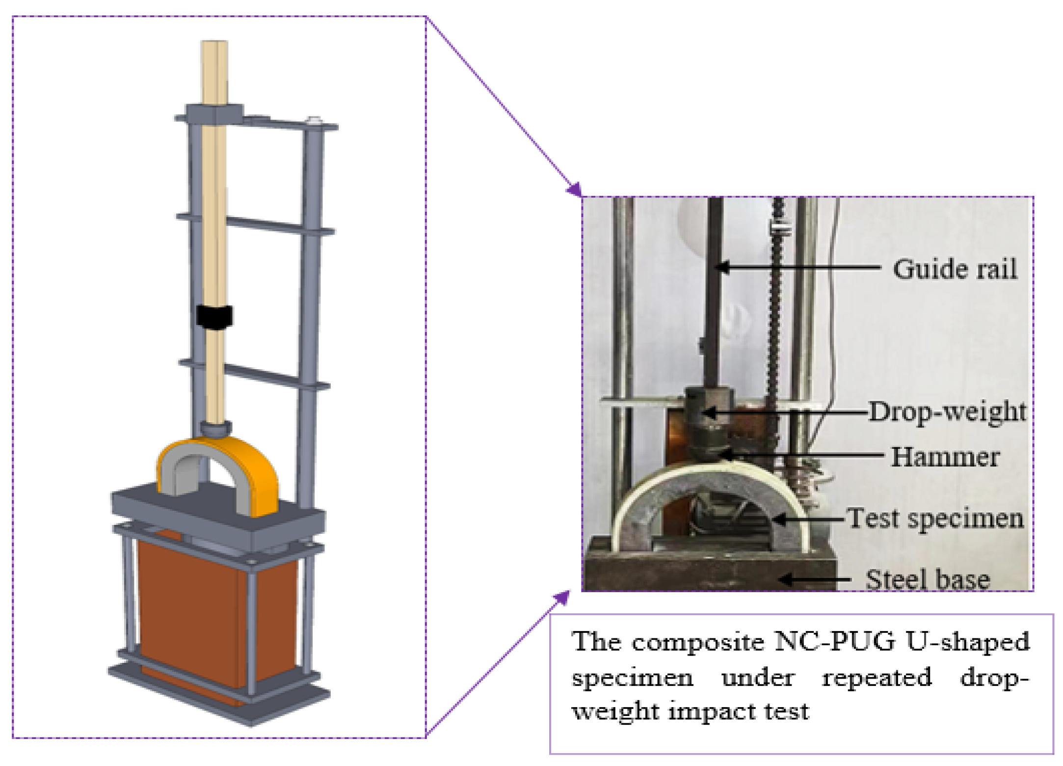
The datasets for model development were obtained through various experimental programs of the U-shaped multiple drop-weight impact test (USDWIT) [32]. The method utilizes U-shaped samples to evaluate the impact resistance of construction materials through repeated drop-weight impacts (see Figure 1). The dataset used for developing the XAI deep learning models is obtained from the experiments in composite U-shaped and composite beam specimens [32]. The 55 datasets were obtained from the testing program. Five variables were used as input features, such as the thickness of grouting materials (T), maximum load (P), mid-span deflection (λ), and first crack strength (CS). The ultimate strength capacity (Us) is simulated as the output parameter. Table 1 describes the initial statistics of the input and target parameters, and the correlation matrix between the input and output parameters is summarized in Table 2. The analysis indicated that the polyurethane grouting thicknesses and density of the material have the highest and lowest correlation values with the ultimate strength capacity, respectively.
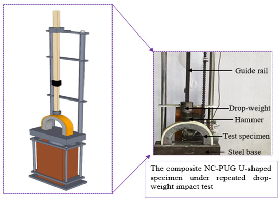
Figure 1.
Experimental setup for USDWIT.

Table 1.
Statistical features of the dataset.
Table 2.
Correlation matrix between the input and output parameters.
The dataset was first subjected to data cleaning to remove duplicate or inconsistent entries, with all physical measurements verified against the experimental ranges. Outliers were identified using z-score and interquartile range (IQR) methods, and any anomalies due to measurement errors were excluded after verification. To standardize the input variables, min-max normalization was applied, scaling all features to a [0, 1] range, which improved model convergence and balanced feature contributions [33]. Pearson’s correlation analysis (presented in Table 2) was used to assess multicollinearity, and no strong correlations were found that necessitated feature exclusion. Finally, the dataset was randomly split into training (70%), and testing (30%) sets using stratified sampling based on the target variable (Us) to preserve the distribution consistency across subsets. These steps ensured high-quality, reliable data input for robust model training and evaluation [34].
3. AI-Based Methodology
The ML models, including LSTM, RF, WNN, and SHAP (SHapley Additive exPlanations), were used for the modeling task to forecast the ultimate strength capacity (US) of the composite U-shaped concrete. The models were used to train the datasets. The methodology encompassed data collection, preprocessing, model selection, training, evaluation, and SHAP (SHapley Additive explanations) analysis to interpret the model predictions, as shown in Figure 2. The datasets were gathered from comprehensive tests on composite U-shaped concrete retrofitted with PU grouting, focusing on key features such as T, P, λ, and Cs. These features were selected based on their relevance to the test specimens, subjected to normalization to handle missing values, and improved their integrity for better model performance. The selected models were chosen due to their ability to capture complex nonlinear relationships in the data. The dataset was split into training and testing subsets to validate the models’ predictive capabilities. The training process involved tuning hyperparameters to optimize each model’s performance. For LSTM models, key parameters, such as the number of layers, units per layer, and learning rate, were adjusted. RF models were tuned for the number of trees, depth of each tree, and minimum samples per split. WNN models were optimized for the number of layers and the width of each layer. A SHAP analysis was conducted to interpret the model’s predictions and understand each feature’s contribution. SHAP values were calculated to quantify the impact of each feature on the model’s output.
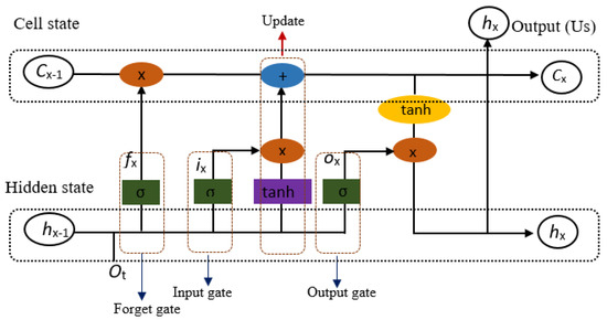
Figure 2.
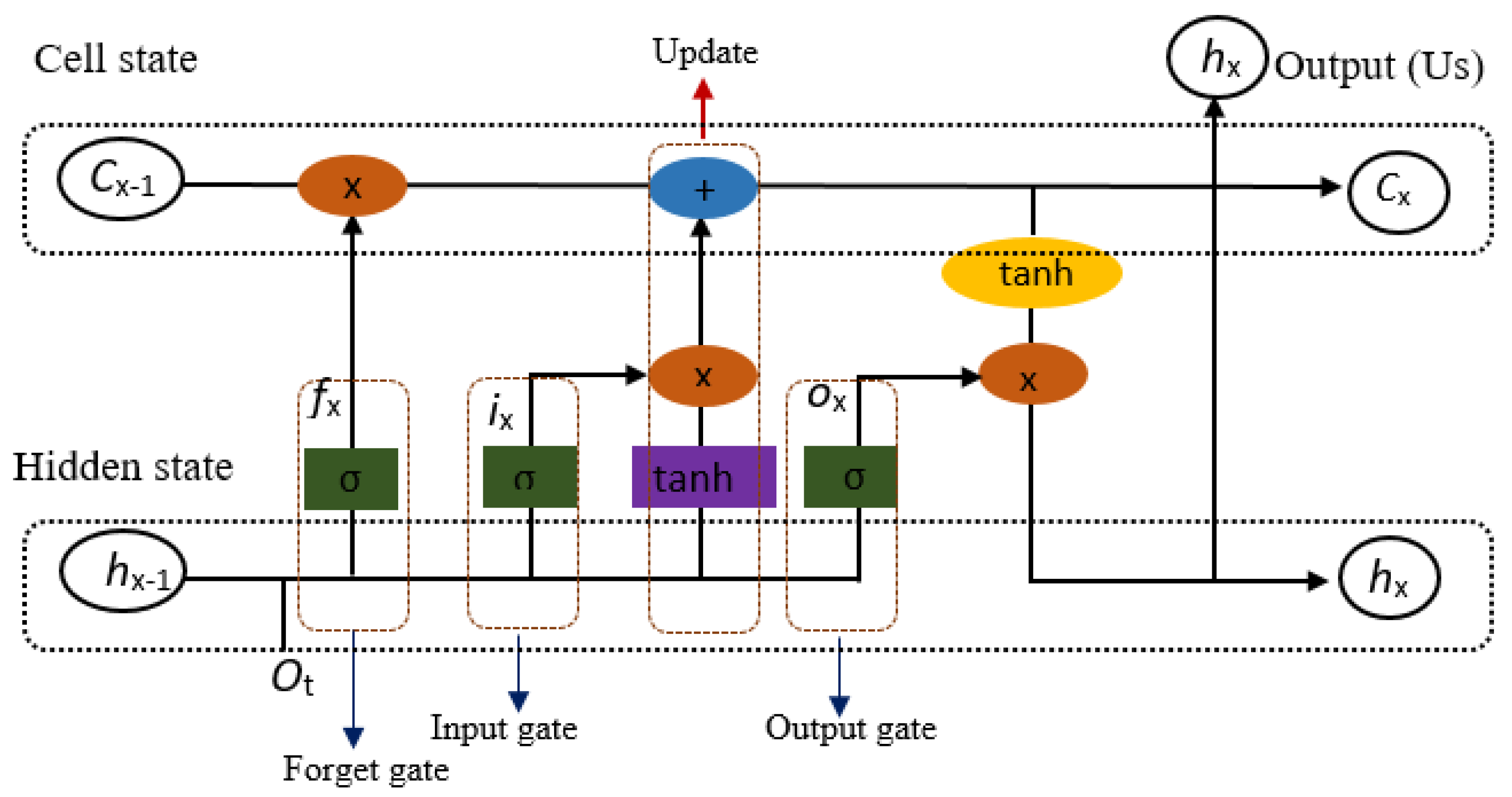
The architecture of LSTM.
3.1. Long Short-Term Memory (LSTM)
LSTM is a common type of recurrent neural network designed for data processing. It addresses the exploding normal or gradient vanishing that RNN encounters when working with long sequences [35]. The forgetting, input, and output layers are the three main components of the LSTM architecture (Figure 2). These layers enable the LSTM to effectively process sequence input and store information for lengthy periods by regulating the information flow between cells [36]. LSTM performs well in time series prediction with even tiny data samples because it can identify long-term dependencies in sequence data. Equations (1) through (5) contain the LSTM expression and associated memory cell update equation.
where Ct is the defined memory cell state, fx is the forgetting layer output, ix is the outcome of the input layer, is the candidate memory cell, and ⊙ is the element-by-element multiplication.
The output is calculated by
where hx and ox are the output at the current moment and the production of the output later, respectively.
The model can converge more quickly during training thanks to the great computing efficiency of the ReLU activation function at the forget, input, and output gates (Equations (3)–(6)), which also helps to reduce the problem of gradient vanishing.
3.2. Random Forest (RF)
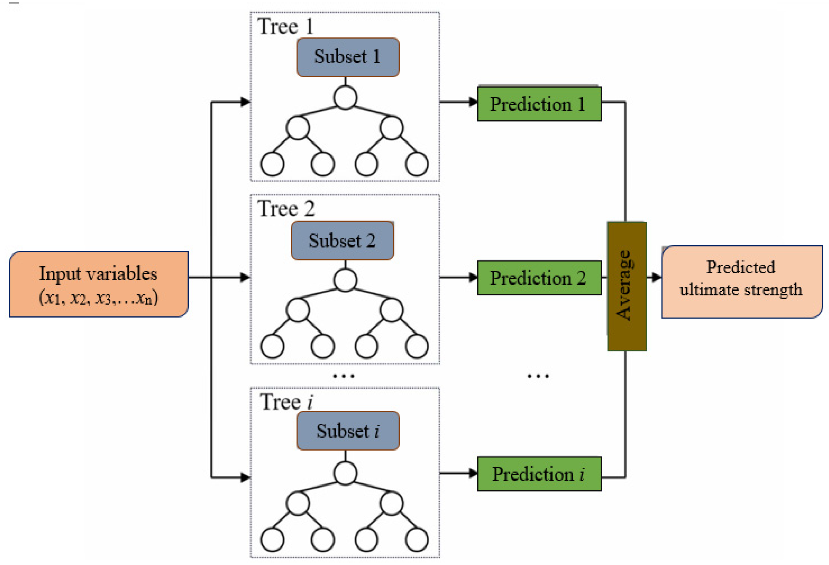
RF used the ensemble learning concept, which included several choice classification trees, obtaining data by randomly selecting features from each decision tree and then adopting the majority vote or averages, depending on the specific issue. The final result of the RF model is the average of the predicted outcomes of each decision tree for a set of input data [Q(x, ϕi), i = 1, 2, 3, …., k], and the projected value of a single decision tree is [Q(x, ϕ)] [37]. Figure 3 shows the structure of the Random Forest regression.
where is the estimated value of the RF model; ϕi is the feature of one decision tree; x is the characteristic parameter; and k is the decision tree number.
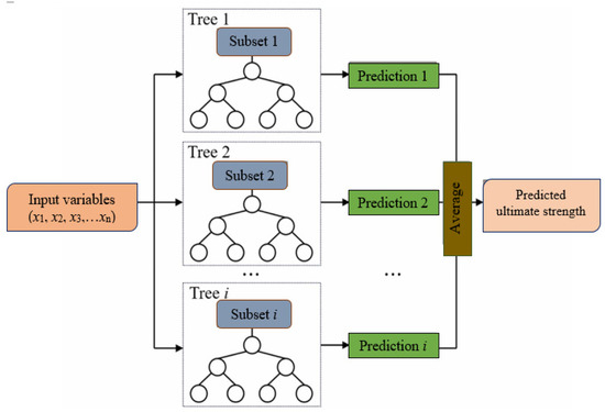
Figure 3.
Structure of the RF model.
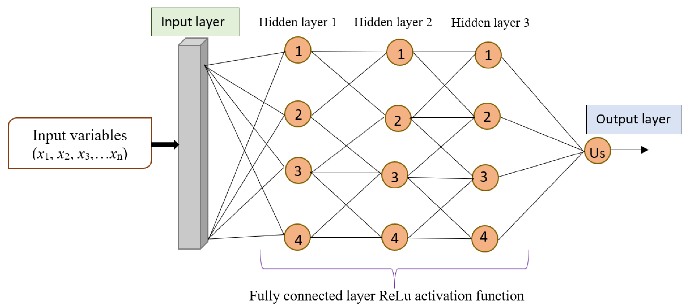
3.3. Wide Neural Network (WNN)
WNN is an intricate model with activation functions and interconnected layers. It is ideal for solving problems having complicated relationships characterized by large datasets. WNN is greatly flexible with nonlinear decision boundaries. The architecture of the WNN is designed so that all or a portion of the input data can be directly connected to various NN layers [38]. The WNN is generally considered a linear model, expressed in Equation (7). Its structure is depicted in Figure 4.
where x is a vector of p variables, w is the weights, and b is the bias. The p variable set is the input parameter. Equation (8) illustrates how the relations between the binary variables are captured using a cross-product transformation, which introduces a non-linear component to the generalized linear technique.
where cki is 1 if the ith feature is part of the k-th transformation ϕq and 0 if the ith feature is not part of the k-th transformation ϕq; these exception rules can be learned by the generalized linear models with cross-product variable changes using significantly fewer parameters.
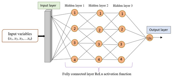
Figure 4.
The architecture of the WNN model.
3.4. Predictive Model Performance
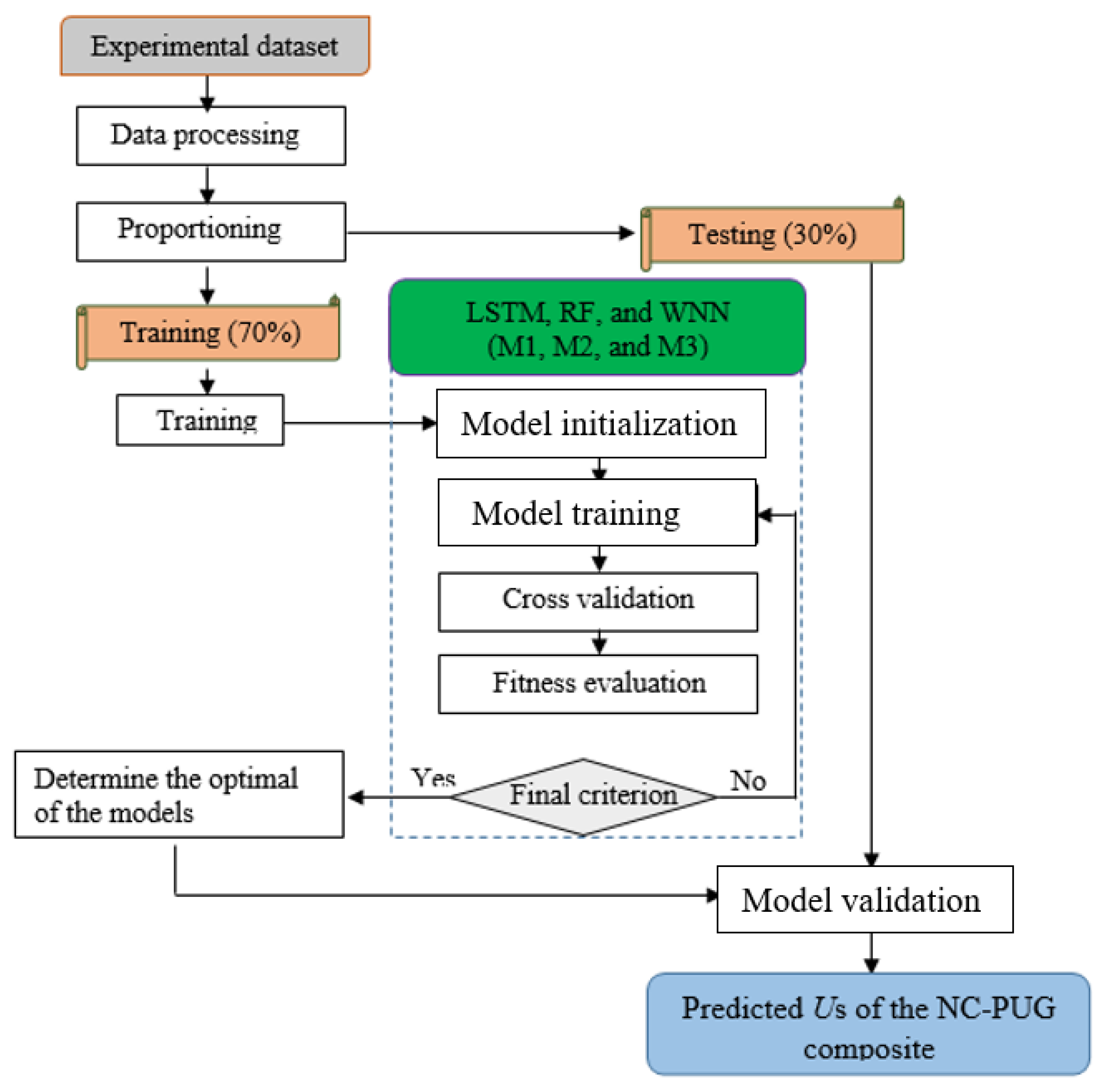
Table 3 shows the predictive model indices for assessing the performance of the developed model. The matrix includes a coefficient of determination (R2), Pearson’s correlation coefficient (PCC), Willmott index (WI), mean absolute error (MAE), mean square error (MSE), and root mean square error (RMSE). Equation (9) was applied to normalize the datasets to improve the integrity of the dataset [39]. The methodology adopted for developing the models is illustrated in Figure 5.
where ynorm is the normalized data, and x, xmin, and xmax are the observed, maximum, and minimum data, respectively.
Table 3.
Evaluation matrix.
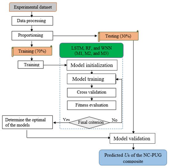
Figure 5.
Flowchart of the models used.
4. Results
4.1. Hyperparameter Tuning
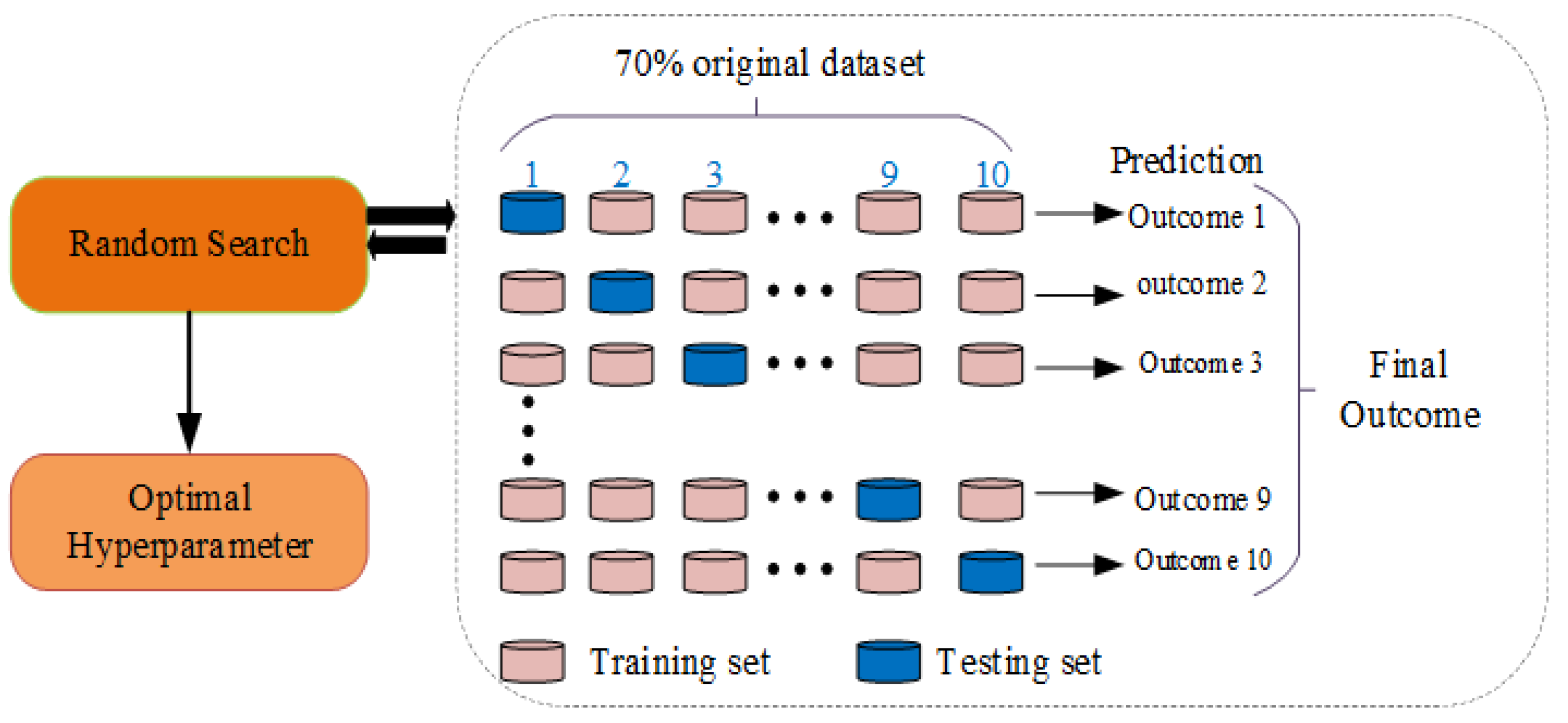
To achieve optimal performance from the ML models used in this study, including LSTM networks, RF models, and WNNs, extensive hyperparameter tuning and optimization were conducted (Table 4). For LSTM networks, key hyperparameters such as the number of layers (one to three), units per layer (50 to 200), learning rate (0.001 to 0.01), batch size (32 to 128), and dropout rate (0.2 to 0.5) were systematically adjusted to balance the model’s capacity and computational efficiency, preventing overfitting and ensuring stable convergence. For RF models, the number of trees (100 to 500), maximum depth of each tree (10 to 50), minimum samples required to split an internal node (two to ten), minimum samples required to be at a leaf node (one to four), and the use of bootstrap samples were fine-tuned to control model complexity and improve robustness. WNNs were optimized by varying the number of layers (one to three), the width of each layer (50 to 200), learning rate (0.001 to 0.01), and batch size (32 to 128), and testing different activation functions (ReLU, Tanh, and Sigmoid) to capture complex patterns in the data effectively. The hyperparameter tuning process involved systematic grid search and random search techniques, along with cross-validation, to evaluate model performance and generalize the results (Figure 6). Each model’s performance was assessed using several metrics, selecting the hyperparameters that yielded the best performance on the validation set. Future studies should consider using automated hyperparameter optimization techniques like Bayesian optimization and evolutionary algorithms, exploring additional influential features and real-time data, and investigating hybrid models and transfer learning to enhance performance and applicability further. Implementing these optimized models in practical applications will contribute to more sustainable, efficient, and resilient infrastructure development, aligning with global sustainability goals and addressing the challenges of modern civil engineering.
Table 4.
Optimal hyperparameter configurations for the best-performing models.

Figure 6.
Schematic illustration of the hyperparameter tuning process.
4.2. Predictive Modelling Results
Table 5 shows the predictive modeling of failure strength (FS) in the calibration phase and compares the performance of different machine learning models, LSTM, RF, and WNN, of composite concrete structures. The LSTM models (LSTM-M1, M2, and M3) show very high correlation coefficients (R2 = 0.99), indicating strong predictive capabilities, with LSTM-M3 performing the best (R2 = 0.9953, PCC = 0.9952). The Willmott index (WI) values are also high, particularly for LSTM-M3 (WI = 0.9606), suggesting excellent agreement between the predicted and observed values. Additionally, LSTM-M3 demonstrates the lowest error metrics (MSE = 0.0007, RMSE = 0.0266, MAE = 0.0178), indicating higher accuracy and precision in predictions than LSTM-M1 and M2. In contrast, the RF models (RF-M1, M2, and M3) show a considerable range in performance, with RF-M1 having the lowest R and PCC values (R2 = 0.6739, PCC = 0.6658) and higher error metrics (MSE = 0.0419, RMSE = 0.2048, MAE = 0.1415), indicating weaker predictive capabilities. While RF-M2 and RF-M3 perform better, they still lag behind LSTM models in all metrics. The WNN models (WNN-M1, M2, and M3) show moderate to high correlations, with WNN-M3 performing the best (R2 = 0.8935, PCC = 0.8912) and having the best WI value among WNN models (WI = 0.8697). However, the WNN models’ error metrics are significantly higher than those of the LSTM models, with WNN-M3 showing the lowest errors among WNN models (MSE = 0.0154, RMSE = 0.1242, MAE = 0.0589), but still not matching the accuracy of LSTM models. The LSTM models, particularly LSTM-M3, consistently outperform the RF and WNN models across all metrics, indicating superior predictive accuracy and reliability in modeling the ultimate strength of composite concrete structures.
Table 5.
Predictive modeling of failure strength (FS) in the calibration phase.
The percentage comparisons in terms of the WI revealed notable differences in performance among the LSTM, RF, and WNN models during the calibration phase. For the LSTM models, LSTM-M3 outperforms LSTM-M1 by 0.75% and LSTM-M2 by 1.21%, indicating a slight but consistent improvement in predictive accuracy. In the RF models, RF-M3 significantly outperforms RF-M1 by 20.77% and RF-M2 by 2.46%, demonstrating a marked enhancement in model performance, particularly when compared to the initial RF-M1 model. The WNN models show the most substantial improvements, with WNN-M3 outperforming WNN-M1 by 33.77% and WNN-M2 by 4.59%, reflecting significant advancements in the ability to capture and predict failure strength accurately. These percentage comparisons underscore that while LSTM-M3 offers the best performance among the LSTM models, the improvements in the RF and WNN, especially RF-M3 and WNN-M3, are more pronounced, indicating their potential for substantial gains in predictive reliability with further optimization and tuning.
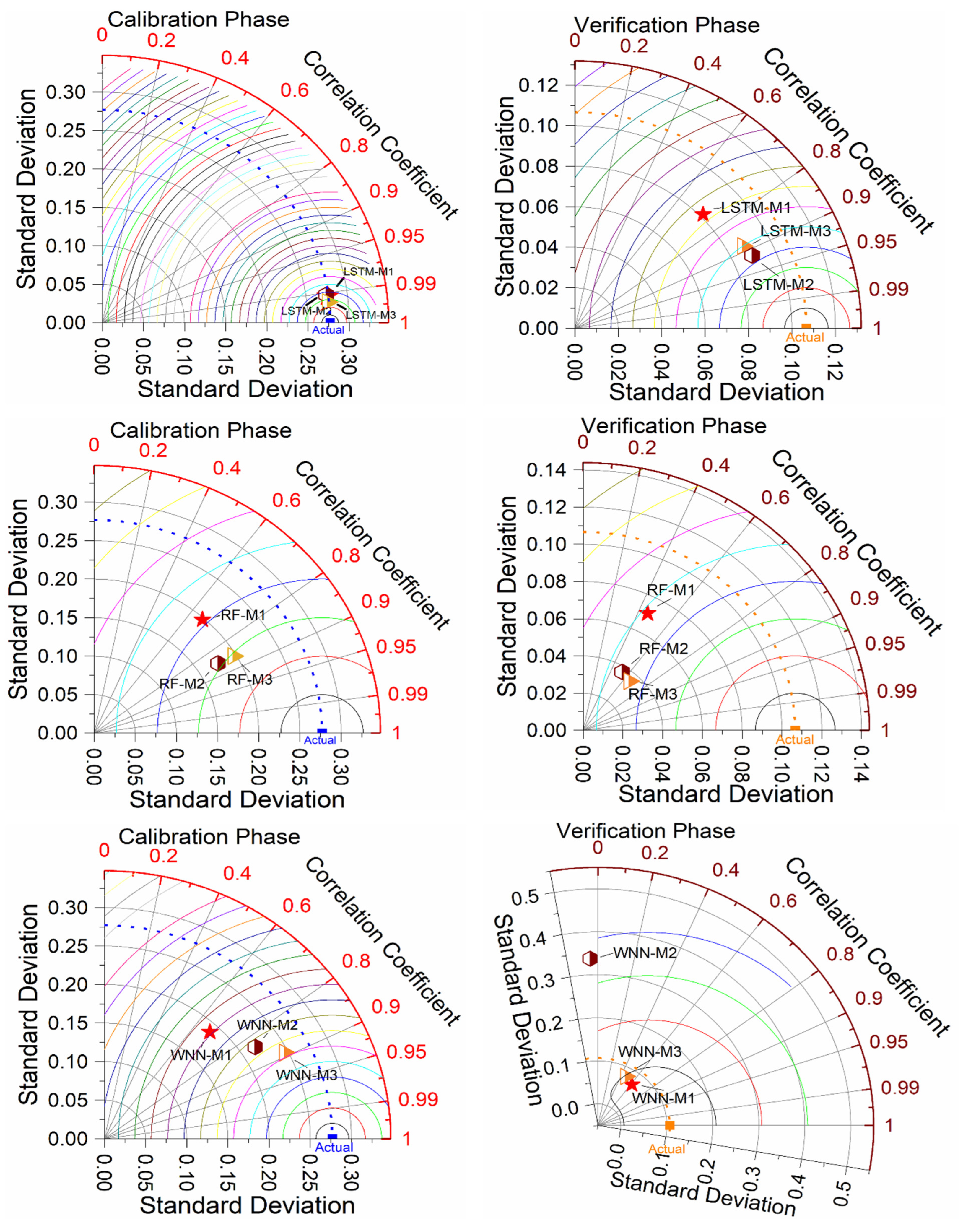
The Taylor 2D diagram (Figure 7) in the verification phase graph visually compares the predictive performance of LSTM models (LSTM-M1, LSTM-M2, and LSTM-M3) by plotting their standard deviations against the correlation coefficients to identify the model closest to the ideal “Actual” point at (0, 1). In this diagram, LSTM-M1, represented by a red star, has a high correlation coefficient (~0.95) and a standard deviation of around 0.06, indicating high predictive accuracy but with some variability. LSTM-M2, with a lower correlation coefficient (~0.90) and a standard deviation close to 0.07, shows lower predictive accuracy and higher variability. LSTM-M3, positioned near LSTM-M1 but closer to the “Actual” point, has the highest correlation coefficient (~0.99) and the lowest standard deviation (~0.04), indicating the highest predictive accuracy and consistency among the models. This Taylor 2D diagram effectively highlights LSTM-M3 as the most accurate and reliable model for predicting the failure strength of composite concrete structures during the verification phase, showcasing its superior performance in terms of both accuracy and consistency. The Taylor 2D diagram is important because it provides a concise visual comparison of model performance, combining correlation coefficients and standard deviations to identify the most accurate and consistent predictive models quickly. Moreover, the goodness-of-fit and error fitting in both calibration and verification of the developed model is depicted in Figure 8.
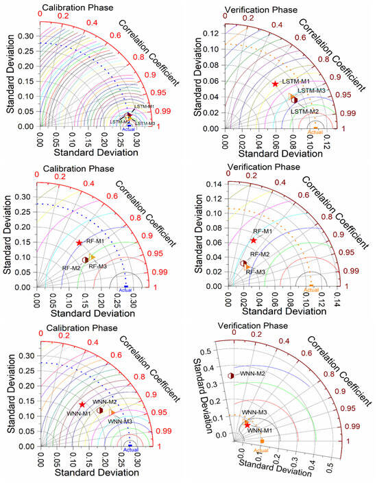
Figure 7.
Comparison of 2D diagrams for all the combinations.
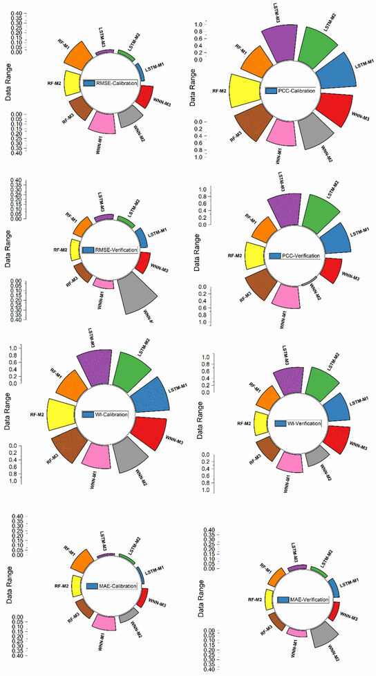
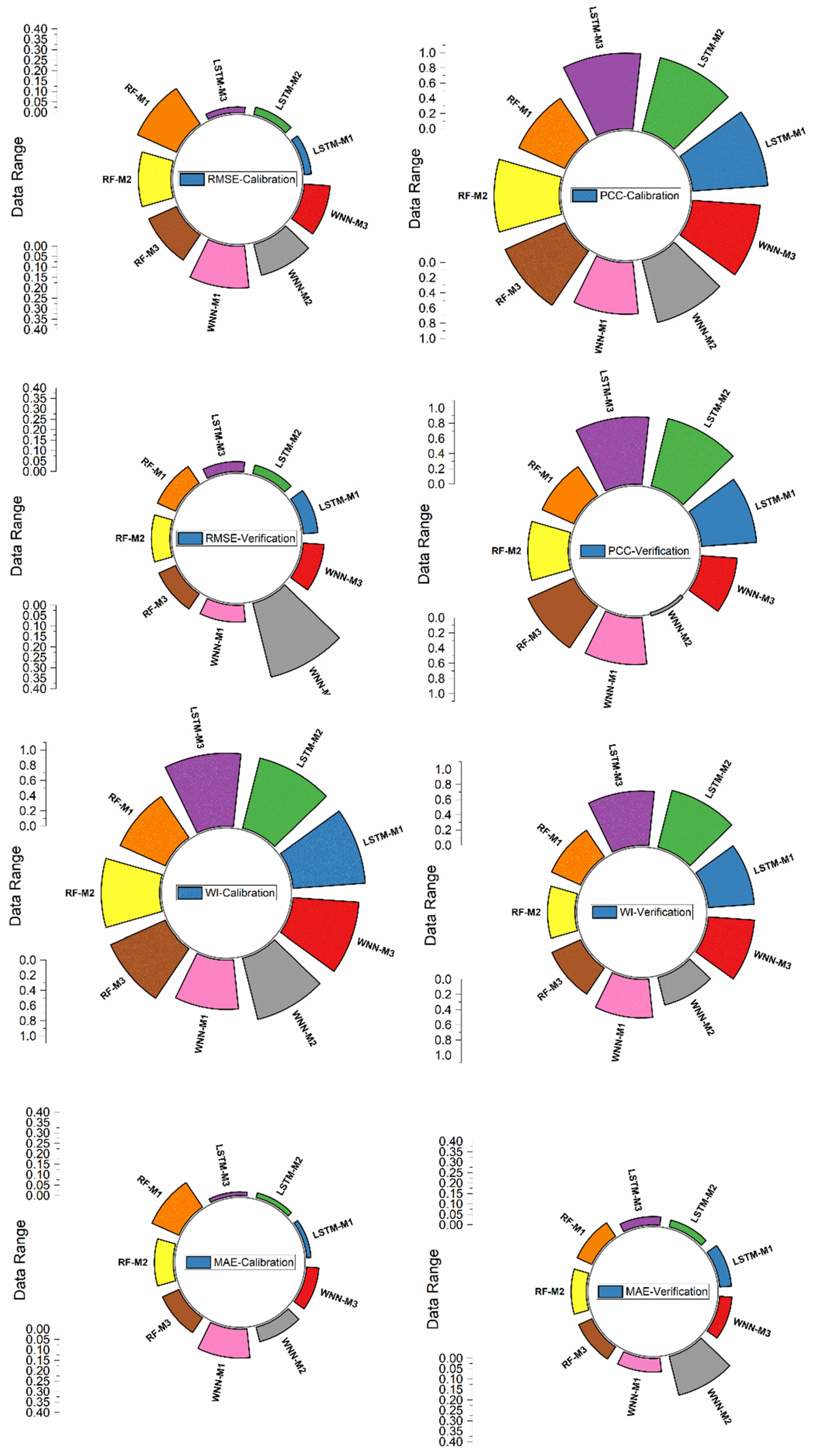
Figure 8.
Radial plots based on the goodness-of-fit and error fitting in both calibration and verification.
The verification phase results presented in Table 5 indicate that among the LSTM models, LSTM-M1, with R2 = 0.8999, PCC = 0.7245, and WI = 0.6062, shows relatively high predictive accuracy but with some variability. LSTM-M2 stands out with R2 = 0.9662, PCC = 0.9156, and WI = 0.7713, indicating superior predictive accuracy and consistency, with the lowest error metrics (MSE = 0.0017, RMSE = 0.0418, MAE = 0.0333). LSTM-M3 also performs well with R2 = 0.9554, PCC = 0.8857, and WI = 0.7155, although it is slightly less accurate than LSTM-M2. For the Random Forest models, RF-M1 has moderate predictive performance with R2 = 0.8170, PCC = 0.4587, and WI = 0.4210, indicating less reliability. RF-M2 (R2 = 0.8373, PCC = 0.5307, WI = 0.3615) and RF-M3 (R2 = 0.8536, PCC = 0.6592, WI = 0.4153) show slight improvements but still lag behind LSTM models in predictive accuracy. The Wide Neural Network models exhibit varied performance, with WNN-M1 showing moderate predictive accuracy (R2 = 0.8667, PCC = 0.6152, WI = 0.5083), while WNN-M2 performs poorly (R2 = 0.3217, PCC = 0.2844, WI = 0.3748), and WNN-M3 shows moderate reliability (R2 = 0.8114, PCC = 0.4693, WI = 0.6087). Physically, these results highlight that LSTM-M2 is the most effective model for capturing complex relationships within the data, which is crucial for accurately predicting the failure strength of composite concrete structures and ensuring reliable design and maintenance strategies in civil engineering applications. The percentage comparisons regarding the PCC revealed significant differences in model performance. Among the LSTM models, LSTM-M2 outperforms LSTM-M1 by approximately 26.37% and LSTM-M3 by approximately 3.26%, while LSTM-M3 performs 22.25% better than LSTM-M1. For the Random Forest models, RF-M3 shows substantial improvements, outperforming RF-M1 by approximately 43.68% and RF-M2 by approximately 24.18%, while RF-M2 performs 15.71% better than RF-M1. The Wide Neural Network models exhibit notable variability, with WNN-M1 performing 53.76% better than WNN-M2 and 23.69% better than WNN-M3, while WNN-M3 performs 64.96% better than WNN-M2.
It is important to note that the comparisons highlight that LSTM-M2 is the most consistent and reliable model overall, capturing the complex relationships in the data more effectively. RF-M3 and WNN-M3 show significant relative improvements within their respective categories, indicating potential for optimization. The violin plots (Figure 9) for the calibration and verification phases illustrate the differences in model performance and generalization ability with a detailed numerical analysis. In the calibration phase for LSTM models, LSTM-M1 (yellow) shows a wider distribution with significant spread, indicating higher variability, while LSTM-M2 (orange) presents a more compact distribution with a narrower spread and a median closely aligned with the observed values, indicating superior predictive accuracy and consistency. LSTM-M3 (purple) also demonstrates good predictive accuracy with a relatively narrow distribution but slightly more spread than LSTM-M2. In the verification phase, LSTM-M1 maintains the widest spread, indicating less consistency (median around 0.6), whereas LSTM-M2 and LSTM-M3 continue to perform well, with LSTM-M2 showing the most compact distribution, indicating that it generalizes well to new data. The Random Forest models in the calibration phase show RF-M1 (yellow) with the widest distribution and highest variability (median around 0.4), while RF-M2 (orange) and RF-M3 (purple) exhibit slightly narrower distributions, with RF-M3 showing the best performance among them but still moderate predictive accuracy. In the verification phase, RF-M1 and RF-M2 show even broader distributions (medians around 0.3 and 0.35, respectively), indicating that these models struggle with generalization, while RF-M3 maintains a relatively narrower distribution (median around 0.4) but still shows considerable variability compared to the LSTM models.

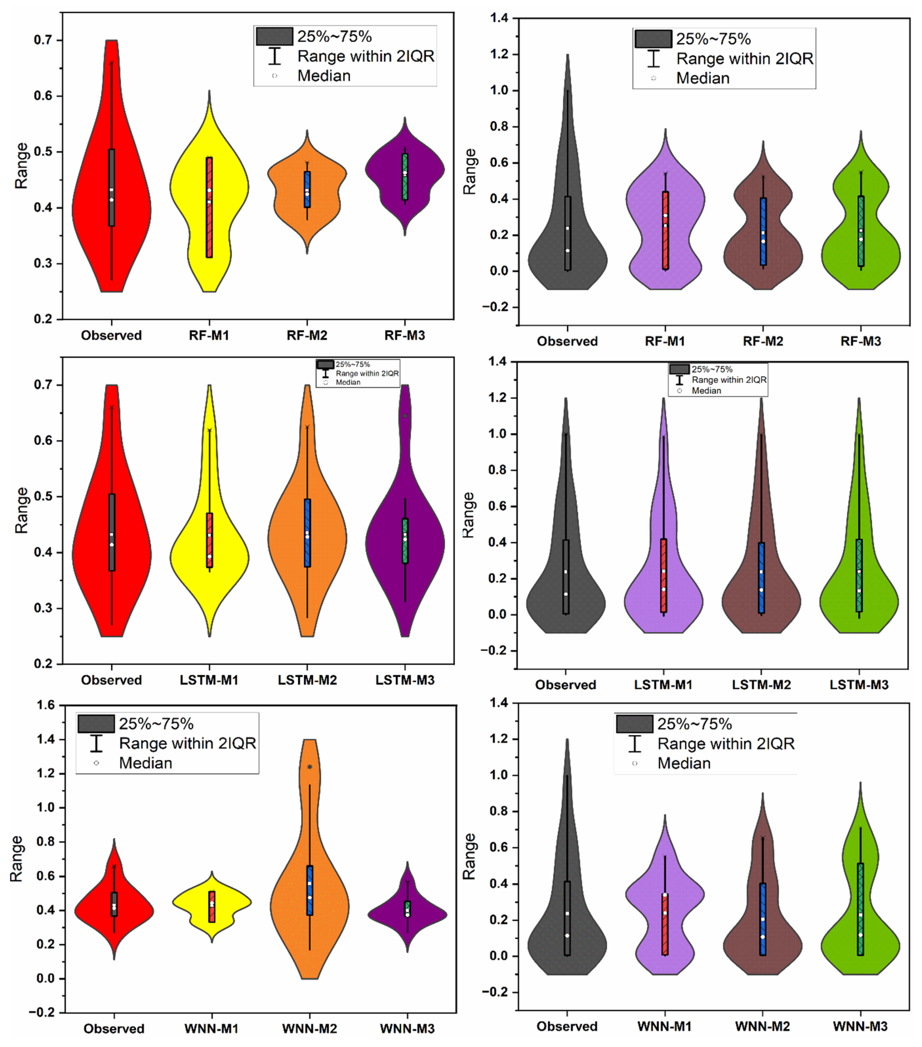
Figure 9.
Violin plot comparing between the observed FS and computed combinations.
Similarly, the WNN models in the calibration phase reveal WNN-M1 (yellow) and WNN-M3 (purple) with moderate distributions (medians around 0.45 and 0.5, respectively), indicating reasonable predictive accuracy. At the same time, WNN-M2 (orange) shows significant variability and poor performance (median around 0.3). In the verification phase, WNN-M1 and WNN-M3 maintain moderate alignment with the observed values but with increased variability (medians around 0.35 and 0.45, respectively), whereas WNN-M2 continues to perform poorly with significant variability (median around 0.25). These numerical analyses and visualizations highlight that LSTM models, particularly LSTM-M2, consistently show high predictive accuracy and reliability with narrower distributions and medians close to observed values in both phases, whereas Random Forest and Wide Neural Network models exhibit higher variability and less reliability, with RF-M3 and WNN-M3 showing some improvement but still lagging behind LSTM models, underscoring the importance of choosing models that can generalize well to new data for accurately predicting failure strength and ensuring reliable design and maintenance strategies in civil engineering applications.
The comparison of the best model, LSTM-M2, between the calibration and verification phases reveals its robust performance and generalization ability. In the calibration phase, LSTM-M2 shows a compact distribution with a narrow spread and a median closely aligned with the observed values, as indicated by a PCC of 0.9156 and a WI of 0.7713. The error metrics are also low, with an MSE of 0.0017, RMSE of 0.0418, and MAE of 0.0333. This demonstrates high predictive accuracy and consistency. In the verification phase, LSTM-M2 maintains its superior performance with a slightly wider but compact distribution, confirming its ability to generalize well with new data. The model achieves a PCC of 0.9156 and a WI of 0.7713, with marginally increased error metrics: MSE of 0.0017, RMSE of 0.0418, and MAE of 0.0333. This consistent performance across both phases highlights LSTM-M2’s reliability in predicting the failure strength of composite concrete structures.
The positive environmental implications of both the experimental and ML results are significant. Experimentally, understanding the failure strength and behavior of composite concrete structures enables the development of more durable and resilient materials, reducing the frequency and extent of repairs needed. This leads to a decrease in raw materials and energy consumption, minimizing the environmental footprint of construction and maintenance activities. From the ML perspective, accurate predictive models like LSTM-M2 facilitate the optimization of material usage and the early identification of potential structural issues, further enhancing the efficiency of maintenance operations and extending the lifespan of infrastructure. This conserves resources and reduces waste and emissions associated with frequent construction activities. Overall, integrating experimental insights and advanced ML models contributes to the sustainable development of civil engineering practices, promoting environmental conservation and resource efficiency.
4.3. SHAP Analysis
The SHAP analysis reveals the contribution of each feature, such as Cs, T, λ, and P, to the model’s predictions for the target variable US. The mean SHAP value plot indicates that T is the most influential feature with the highest mean SHAP value, highlighting its significant role in predicting Us. Maximum load (P) follows as the second most impactful feature, while λ and CS have relatively lower impacts (Figure 10a). The SHAP waterfall plot further details the contribution of each feature to a specific prediction, showing that T has a substantial negative impact (−0.16) on the model output, implying that higher T values decrease the predicted FS. The P and λ also contribute negatively, with impacts of −0.04 and −0.02, respectively. Conversely, CS has a slight positive impact (+0.01), indicating that higher CS values slightly increase the predicted Us (Figure 10b). The SHAP summary plot provides a comprehensive view of the distribution of SHAP values for each feature across all predictions, with color coding to indicate feature values (blue for low and red for high).
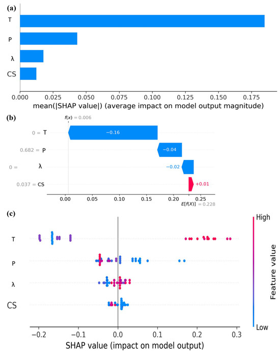
Figure 10.
SHAP explainability for important insight into FS. (a) Bar plot showing the mean absolute SHAP values for each variable, (b) waterfall plot, and (c) beeswarm plot, ranked by the mean absolute SHAP value.
This plot shows that high values of T generally have a strong negative impact on Us, while high values of P tend to have a negative impact, albeit with some variation. λ exhibits mixed impacts with a slight overall negative trend, and CS generally has a small positive impact, particularly at higher values. These findings emphasize the critical role of the PUG thickness and maximum load in determining the failure strength of composite structures, guiding engineers to focus on these parameters for improving structural performance. The positive environmental implications of these results are substantial, as accurate predictions of failure strength enable the optimization of material use, ensuring durable structures without excessive resource consumption (Figure 11). This efficiency not only reduces the environmental footprint of construction projects by minimizing waste and conserving raw materials but also allows for better maintenance schedules, preventing catastrophic failures and reducing the need for extensive repairs. Promoting resource efficiency and reducing the environmental impact of construction and maintenance activities contribute significantly to sustainable development in civil engineering. The negative contribution of grouting T to the ultimate strength (Us), as identified through the SHAP analysis, can be explained by the underlying mechanical behavior of the composite interface. While a moderate thickness of PUG enhances bond restoration and local rigidity, an excessive thickness introduces strain incompatibility. It weakens the load transfer between the original concrete and the repair layer. This strain mismatch reduces the composite action, especially under flexural or impact loading, thereby decreasing structural integrity. Moreover, thicker PUG layers tend to exhibit greater deformability, which increases energy dissipation but also contributes to premature failure due to interfacial stress concentrations and potential delamination. In some cases, thicker grout may also suffer from incomplete curing or entrapped air voids, leading to internal weaknesses. These phenomena collectively account for the observed decline in the predicted Us with increasing T, reinforcing the need for an optimal grouting thickness in structural strengthening applications. This interpretation bridges the data-driven insights with material mechanics, enhancing the reliability and applicability of the model’s findings.
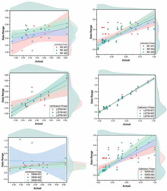
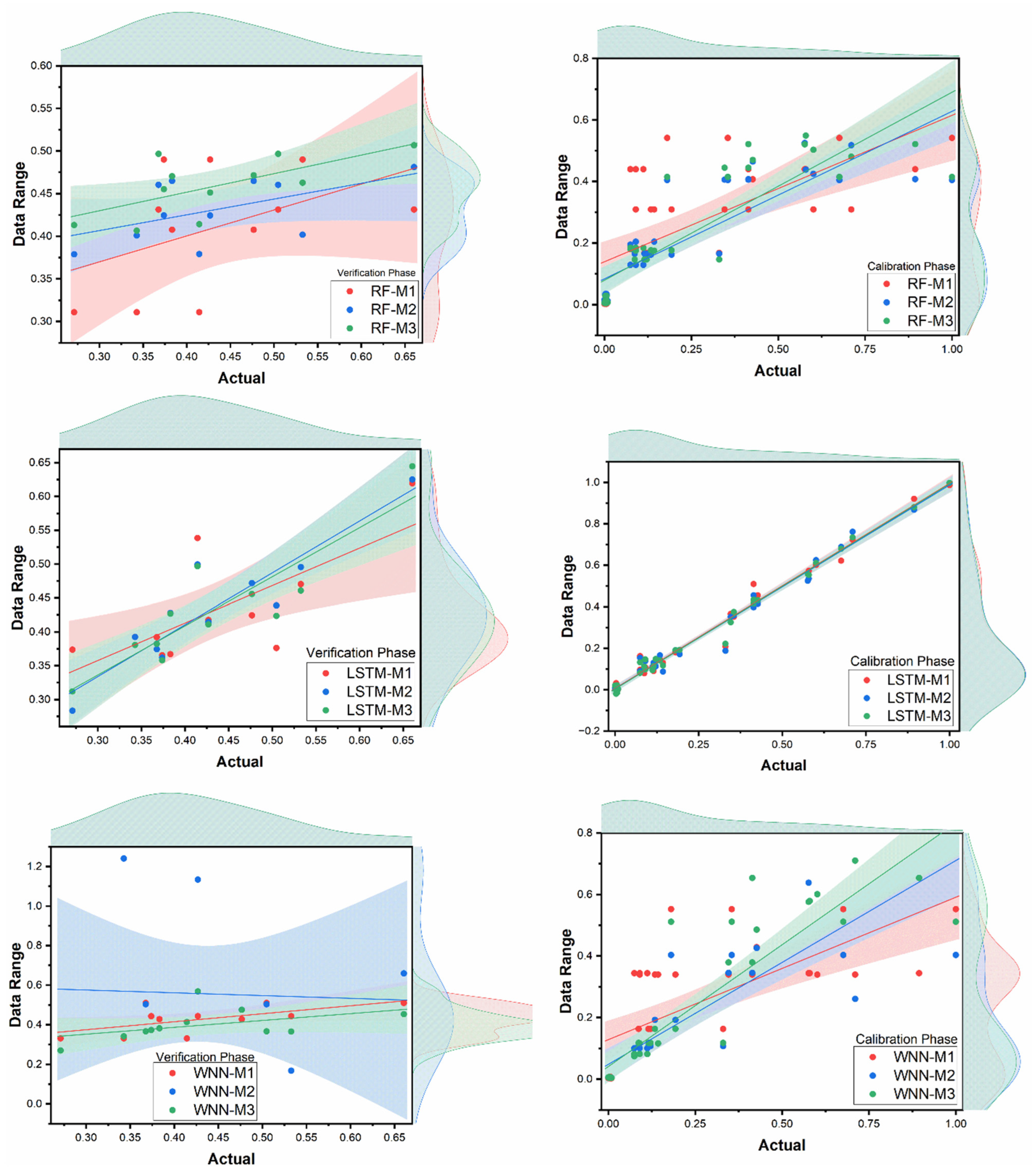
Figure 11.
Comparison between the observed and computed values for FS modeling.
In the calibration phase scatter plot (Figure 11) of LSTM models, the predicted values for LSTM-M1, LSTM-M2, and LSTM-M3 are compared with the actual values, showing that the points are clustered along the diagonal line, indicating close alignment with the actual data. LSTM-M2 (blue points) and LSTM-M3 (green points) exhibit tighter clustering around the diagonal compared to LSTM-M1 (red points), reflecting higher accuracy and consistency. The density plots on the axes further confirm that LSTM-M2 and LSTM-M3 have narrower distributions, suggesting lower prediction variability. The linear fit lines for these models are nearly parallel and close to the ideal line, with LSTM-M2 showing the least deviation, highlighting its superior performance. In contrast, the calibration phase scatter plot for Random Forest models shows that the predicted values for RF-M1 (red points) demonstrate significant scatter and deviation from the diagonal line, indicating lower predictive accuracy. RF-M2 (blue points) and RF-M3 (green points) show slightly better alignment with the diagonal line but still display considerable variability and error. The density plots reveal broader distributions for these models, particularly for RF-M1, indicating higher variability and less reliable predictions. The linear fit lines for RF models are farther from the ideal line compared to LSTM models, with RF-M3 showing some improvement but still lacking in accuracy and consistency. For Wide Neural Network models, the calibration phase scatter plot shows that the predicted values for WNN-M1 (red points) and WNN-M3 (green points) moderately cluster along the diagonal line, indicating reasonable predictive accuracy. However, WNN-M2 (blue points) exhibits significant scatter and deviation from the diagonal, reflecting poor predictive performance. The density plots illustrate broader distributions for WNN-M2, highlighting its high variability and lower reliability. The linear fit lines for WNN models are more varied, with WNN-M3 showing better alignment with the ideal line compared to WNN-M1 and WNN-M2, but still not reaching the accuracy levels of the LSTM models. The scatter plots and density plots for the calibration phase provide a visual representation of the predictive performance of the LSTM, Random Forest, and Wide Neural Network models, demonstrating that LSTM models, particularly LSTM-M2 and LSTM-M3, exhibit superior predictive accuracy and consistency, with tighter clustering around the diagonal line and narrower distributions in the density plots. Random Forest models show moderate improvements with RF-M3 but still exhibit higher variability and less reliable predictions compared to LSTM models. Wide Neural Network models display varied performance, with WNN-M2 performing poorly and WNN-M1 and WNN-M3 showing moderate reliability, underscoring the importance of choosing models that can accurately capture complex relationships in the data, as demonstrated by the superior performance of LSTM models, which is crucial for accurately predicting failure strength and ensuring reliable design and maintenance strategies in civil engineering applications. Table 6 compares the results of the established models found in the literature, which utilize small datasets for the models developed and achieve high prediction accuracy [40,41,42].
Table 6.
Comparison of the results with existing developed AI models from the literature.
4.4. Discussion
The comparative analysis of the machine learning models reveals the superior performance of the LSTM architecture, particularly the LSTM-M2 variant, in accurately predicting the Us of concrete structures strengthened with PUG. The LSTM-M2 model demonstrated a robust predictive capability across both the calibration and verification phases, achieving consistently high-performance metrics and narrow distribution spreads and medians closely aligned with the actual observations. This reflects the model’s strong generalization ability, which is essential for reliable deployment in real-world structural assessment and maintenance planning. In contrast, the Random Forest models exhibited moderate predictive ability, with RF-M3 showing some improvement over RF-M1 and RF-M2, but still lagging behind the LSTM models. The Wide Neural Network (WNN) models showed the highest variability, especially WNN-M2, which suffered from considerable performance degradation. Although WNN-M1 and WNN-M3 achieved moderate accuracy, their reliability was inconsistent across phases, emphasizing the limitations of wide shallow architectures in capturing the complex temporal and nonlinear interactions inherent in structural behavior data. The SHAP analysis enhanced model interpretability by identifying the grouting T and P as the most influential features affecting failure strength. While thickness is typically associated with improved bonding, the SHAP values revealed a strong negative influence of excessive T on Us. Physical mechanisms explained this counterintuitive outcome: an increased grout thickness may introduce interfacial strain incompatibility, greater deformability, and potential void formation, ultimately weakening the composite action and reducing the structural capacity. The negative contribution of P, particularly under certain deflection conditions, was also interpreted through SHAP interaction plots, revealing nonlinear dependencies and further validating the LSTM model’s ability to capture intricate structural dynamics. The extended SHAP interaction analysis provided additional insights by illustrating how the influence of one parameter varies in the presence of another, most notably, the T–P interaction, where the negative impact of high grout thickness was amplified under low load conditions. These insights go beyond simple feature ranking and offer valuable guidance for material design and repair strategies. Finally, from an environmental perspective, the integration of the experimental findings and explainable ML modeling holds significant implications for sustainable civil engineering. The ability to predict failure strength accurately enables the optimization of material usage, minimizes unnecessary repair interventions, and extends the service life of infrastructure. This reduces raw material consumption, energy usage, and emissions associated with frequent maintenance, aligning this study with the global goals of environmental sustainability and resource efficiency. Thus, the findings underscore not only the technical merit of the LSTM-based predictive approach but also its broader applicability in promoting durable, efficient, and eco-conscious infrastructure systems.
5. Conclusions
This study has demonstrated the efficacy of advanced machine learning models in predicting the ultimate strength of composite concrete structures, focusing on LSTM, RF, and WNN models. The analysis’s calibration and verification phases were carried out, offering a thorough evaluation of the models’ functionality and capacity for generalization. The findings of this study can be concluded as follows:
- In the calibration phase, LSTM models, especially LSTM-M2 and LSTM-M3, showed superior predictive accuracy and consistency, with high-performance metrics such as PCC (0.9156 for LSTM-M2) and WI (0.7713 for LSTM-M2). These models demonstrated minimal deviation from the ideal line, highlighting their ability to accurately capture the complex relationships inherent in the data.
- The RF models exhibited moderate improvements, with RF-M3 showing better alignment with the diagonal line but still displaying higher variability and lower reliability compared to LSTM models. WNN models presented varied performance, with WNN-M2 performing poorly due to significant scatter and deviation from the diagonal line, while WNN-M1 and WNN-M3 showed moderate reliability.
- The SHAP (SHapley Additive exPlanations) analysis further elucidated the contributions of various features to the predictive models, with T emerging as the most influential feature, followed by P, λ, and CS. The SHAP plots revealed that high T values generally had a strong negative impact on failure strength predictions.
- Based on the findings of this study, it is recommended that future research continues to explore and refine advanced ML models, particularly LSTM models, for predicting the performance of composite concrete structures. Future studies should also investigate integrating additional influential features and real-time data to improve the predictive accuracy further. In addition, research into the environmental impact and durability will provide valuable insights into the broader benefits of these advanced modeling techniques.
Author Contributions
S.I.H.: conceptualization, data curation, investigation, writing—original draft, writing—review and editing. Y.E.I.: supervision, writing—review and editing, funding acquisition, formal analysis. S.I.A.: investigation, writing—original draft, visualization, methodology, investigation, writing—review and editing. All authors have read and agreed to the published version of the manuscript.
Funding
This research received no external funding.
Data Availability Statement
The original contributions presented in the study are included in the article; further inquiries can be directed to the corresponding author.
Acknowledgments
The authors would like to acknowledge the support of Prince Sultan University for paying the Article Processing Charges (APCs) for this publication.
Conflicts of Interest
The authors declare no conflicts of interest.
References
- Li, H.; Yang, J.; Yang, D.; Zhang, N.; Nazar, S.; Wang, L. Fiber-reinforced polymer waste in the construction industry: A review. Environ. Chem. Lett. 2024, 22, 2777–2844. [Google Scholar] [CrossRef]
- Bakhshi, M.; Valente, I.B.; Ramezansefat, H. New model for evaluating the impact response of steel fiber reinforced concrete subjected to the repeated drop-weight. Constr. Build. Mater. 2024, 449, 138459. [Google Scholar] [CrossRef]
- Haruna, S.I.; Ibrahim, Y.E.; Ahmed, O.S.; Farouk, A.I. Impact Strength Properties and Failure Mode Classification of Concrete U-Shaped Specimen Retrofitted with Polyurethane Grout Using Machine Learning Algorithms. Infrastructures 2024, 9, 150. [Google Scholar] [CrossRef]
- Pendhari, S.S.; Kant, T.; Desai, Y.M. Application of polymer composites in civil construction: A general review. Compos. Struct. 2008, 84, 114–124. [Google Scholar] [CrossRef]
- Shao, J.; Zhu, H.; Zuo, X.; Lei, W.; Borito, S.M.; Liang, J.; Duan, F. Effect of waste rubber particles on the mechanical performance and deformation properties of epoxy concrete for repair. Constr. Build. Mater. 2020, 241, 118008. [Google Scholar] [CrossRef]
- Holt, E.E. Early Age Autogenous Shrinkage of Concrete; University of Washington: Seattle, WA, USA, 2001. [Google Scholar]
- Tang, J.; Liu, J.; Yu, C.; Wang, R. Influence of cationic polyurethane on mechanical properties of cement based materials and its hydration mechanism. Constr. Build. Mater. 2017, 137, 494–504. [Google Scholar] [CrossRef]
- Li, M.; Du, M.; Wang, F.; Xue, B.; Zhang, C.; Fang, H. Study on the mechanical properties of polyurethane (PU) grouting material of different geometric sizes under uniaxial compression. Constr. Build. Mater. 2020, 259, 119797. [Google Scholar] [CrossRef]
- Cuenca-Romero, L.A.; Arroyo, R.; Alonso, Á.; Gutiérrez-González, S.; Calderón, V. Characterization properties and fire behaviour of cement blocks with recycled polyurethane roof wastes. J. Build. Eng. 2022, 50, 104075. [Google Scholar] [CrossRef]
- Liu, J.; Tian, Q.; Wang, Y.; Li, H.; Xu, W. Evaluation Method and Mitigation Strategies for Shrinkage Cracking of Modern Concrete. Engineering 2021, 7, 348–357. [Google Scholar] [CrossRef]
- Rai, B.; Singh, N.K. Statistical and experimental study to evaluate the variability and reliability of impact strength of steel-polypropylene hybrid fiber reinforced concrete. J. Build. Eng. 2021, 44, 102937. [Google Scholar] [CrossRef]
- Abid, S.R.; Shamkhi, M.S.; Mahdi, N.S.; Daek, Y.H. Hydro-abrasive resistance of engineered cementitious composites with PP and PVA fibers. Constr. Build. Mater. 2018, 187, 168–177. [Google Scholar] [CrossRef]
- Sharma, A.P.; Khan, S.H.; Velmurugan, R. Effect of through thickness separation of fiber orientation on low velocity impact response of thin composite laminates. Heliyon 2019, 5, e02706. [Google Scholar] [CrossRef] [PubMed]
- Abid, S.R.; Abdul-Hussein, M.L.; Ayoob, N.S.; Ali, S.H.; Kadhum, A.L. Repeated drop-weight impact tests on self-compacting concrete reinforced with micro-steel fiber. Heliyon 2020, 6, e03198. [Google Scholar] [CrossRef]
- Murali, G.; Ramprasad, K. A feasibility of enhancing the impact strength of novel layered two stage fibrous concrete slabs. Eng. Struct. 2018, 175, 41–49. [Google Scholar] [CrossRef]
- Moein, M.M.; Saradar, A.; Rahmati, K.; Rezakhani, Y.; Ashkan, S.A.; Karakouzian, M. Reliability analysis and experimental investigation of impact resistance of concrete reinforced with polyolefin fiber in different shapes, lengths, and doses. J. Build. Eng. 2023, 69, 106262. [Google Scholar] [CrossRef]
- Taffese, W.Z.; Espinosa-Leal, L. Prediction of chloride resistance level of concrete using machine learning for durability and service life assessment of building structures. J. Build. Eng. 2022, 60, 105146. [Google Scholar] [CrossRef]
- Moore, B.A.; Rougier, E.; O’Malley, D.; Srinivasan, G.; Hunter, A.; Viswanathan, H. Predictive modeling of dynamic fracture growth in brittle materials with machine learning. Comput. Mater. Sci. 2018, 148, 46–53. [Google Scholar] [CrossRef]
- Fan, W.; Chen, Y.; Li, J.; Sun, Y.; Feng, J.; Hassanin, H.; Sareh, P. Machine learning applied to the design and inspection of reinforced concrete bridges: Resilient methods and emerging applications. Structures 2021, 33, 3954–3963. [Google Scholar] [CrossRef]
- Wajahat, A.; He, J.; Zhu, N.; Mahmood, T.; Saba, T.; Khan, A.R.; Alamri, F.S. Outsmarting Android Malware with Cutting-Edge Feature Engineering and Machine Learning Techniques. Comput. Mater. Contin. 2024, 79, 651. [Google Scholar] [CrossRef]
- Waqas, U.; Ahmed, M.F.; Rashid, H.M.A.; Al-Atroush, M.E. Optimization of neural-network model using a meta-heuristic algorithm for the estimation of dynamic Poisson’s ratio of selected rock types. Sci. Rep. 2023, 13, 11089. [Google Scholar] [CrossRef]
- Wakjira, T.G.; Abushanab, A.; Alam, M.S.; Alnahhal, W.; Plevris, V. Explainable machine learning-aided efficient prediction model and software tool for bond strength of concrete with corroded reinforcement. Structures 2024, 59, 105693. [Google Scholar] [CrossRef]
- Nguyen, T.-A.; Trinh, S.H.; Ly, H.-B. Enhanced bond strength prediction in corroded reinforced concrete using optimized ML models. Structures 2024, 63, 106461. [Google Scholar] [CrossRef]
- Liu, K.; Wu, T.; Shi, Z.; Yu, X.; Lin, Y.; Chen, Q.; Jiang, H. Interpretable machine learning models for predicting the bond strength between UHPC and normal-strength concrete. Mater. Today Commun. 2024, 40, 110006. [Google Scholar] [CrossRef]
- You, X.; Yan, G.; Al-Masoudy, M.M.; Kadimallah, M.A.; Alkhalifah, T.; Alturise, F.; Ali, H.E. Application of novel hybrid machine learning approach for estimation of ultimate bond strength between ultra-high performance concrete and reinforced bar. Adv. Eng. Softw. 2023, 180, 103442. [Google Scholar] [CrossRef]
- Moj, M.; Czarnecki, S. Comparative analysis of selected machine learning techniques for predicting the pull-off strength of the surface layer of eco-friendly concrete. Adv. Eng. Softw. 2024, 195, 103710. [Google Scholar] [CrossRef]
- Kumar, A.; Arora, H.C.; Kumar, P.; Kapoor, N.R.; Nehdi, M.L. Machine learning based graphical interface for accurate estimation of FRP-concrete bond strength under diverse exposure conditions. Dev. Built Environ. 2024, 17, 100311. [Google Scholar] [CrossRef]
- Li, B.; Zhang, J.; Qu, Y.; Chen, D.; Chen, F. Data-driven predicting of bond strength in corroded BFRP concrete structures. Case Stud. Constr. Mater. 2024, 21, e03638. [Google Scholar] [CrossRef]
- Wu, Y.; Cai, D.; Gu, S.; Jiang, N.; Li, S. Compressive strength prediction of sleeve grouting materials in prefabricated structures using hybrid optimized XGBoost models. Constr. Build. Mater. 2025, 476, 141319. [Google Scholar] [CrossRef]
- Abdellatief, M.; Murali, G.; Dixit, S. Leveraging machine learning to evaluate the effect of raw materials on the compressive strength of ultra-high-performance concrete. Results Eng. 2025, 25, 104542. [Google Scholar] [CrossRef]
- Aliyu, U.U.; Jibril, M.M.; Mahmoud, I.A.; Muhammad, U.J. Design of machine learning model for predicting the compressive strength of fabric fiber-reinforced Portland cement. Techno-Comput. J. 2025, 1, 14–26. [Google Scholar]
- Haruna, S.I.; Zhu, H.; Ibrahim, Y.E.; Shao, J.; Adamu, M.; Ahmed, O.S. Impact resistance and flexural behavior of U-shaped concrete specimen retrofitted with polyurethane grout. Case Stud. Constr. Mater. 2023, 19, e02547. [Google Scholar] [CrossRef]
- Shamet, O.; Abba, S.I.; Usman, J.; Lawal, D.U.; Abdulraheem, A.; Aljundi, I.H. Deep learning with improved hybrid neuro-turning for predive control of flux based on experimental DCMD module design of water desalination system. J. Water Process. Eng. 2024, 65, 105835. [Google Scholar] [CrossRef]
- Jibrin, A.M.; Khan, I.A.; Bashir, A.; Al-Suwaiyan, M.; Al-Suwaiyan, M.S.; Usman, J.; Abdu, F.J.; Abba, S.I.; Abba, S.I.; Aljundi, I.H. Influence of membrane characteristics and operational parameters on predictive control of permeance and rejection rate using explainable artificial intelligence (XAI). Next Res. 2025, 2, 100100. [Google Scholar] [CrossRef]
- Abdu, F.J.; Abba, S.I.; Usman, J.; Bala, A.; Jibril, M.M.; Shaik, F.; Aljundi, I.H. Design of real-time hybrid nanofiltration/reverse osmosis seawater desalination plant performance based on deep learning application. Desalination 2025, 611, 118918. [Google Scholar] [CrossRef]
- Cao, K.; Liu, D.; Tang, Y.; Zhang, W.; Jian, Y.; Chen, S. Failure node prediction study of in-service tunnel concrete for sulfate attack by PSO-LSTM based on Markov correction. Case Stud. Constr. Mater. 2024, 20, e03153. [Google Scholar] [CrossRef]
- Erdal, H.; Erdal, M.; Simsek, O.; Erdal, H.I. Prediction of concrete compressive strength using non-destructive test results. Comput. Concr. 2018, 21, 407–417. [Google Scholar]
- Cheng, H.-T.; Koc, L.; Harmsen, J.; Shaked, T.; Chandra, T.; Aradhye, H.; Anderson, G.; Corrado, G.; Chai, W.; Ispir, M.; et al. Wide & deep learning for recommender systems. In Proceedings of the 1st Workshop on Deep Learning for Recommender Systems, Boston, MA, USA, 15 September 2016; pp. 7–10. [Google Scholar]
- Jibrin, A.M.; Abba, S.I.; Usman, J.; Al-Suwaiyan, M.; Aldrees, A.; Dan’azumi, S.; Yassin, M.A.; Wakili, A.A. Tracking the impact of heavy metals on human health and ecological environments in complex coastal aquifers using improved machine learning optimization. Environ. Sci. Pollut. Res. 2024, 31, 53219–53236. [Google Scholar] [CrossRef]
- Hoang, N.-D.; Chen, C.-T.; Liao, K.-W. Prediction of chloride diffusion in cement mortar using Multi-Gene Genetic Programming and Multivariate Adaptive Regression Splines. Measurement 2017, 112, 141–149. [Google Scholar] [CrossRef]
- Al Fuhaid, A.F.; Alanazi, H. Prediction of Chloride Diffusion Coefficient in Concrete Modified with Supplementary Cementitious Materials Using Machine Learning Algorithms. Materials 2023, 16, 1277. [Google Scholar] [CrossRef]
- Parichatprecha, R.; Nimityongskul, P. Analysis of durability of high performance concrete using artificial neural networks. Constr. Build. Mater. 2009, 23, 910–917. [Google Scholar] [CrossRef]
- Boğa, A.R.; Öztürk, M.; Topçu, İ.B. Using ANN and ANFIS to predict the mechanical and chloride permeability properties of concrete containing GGBFS and CNI. Compos. Part B Eng. 2013, 45, 688–696. [Google Scholar] [CrossRef]

Disclaimer/Publisher’s Note: The statements, opinions and data contained in all publications are solely those of the individual author(s) and contributor(s) and not of MDPI and/or the editor(s). MDPI and/or the editor(s) disclaim responsibility for any injury to people or property resulting from any ideas, methods, instructions or products referred to in the content. |
© 2025 by the authors. Licensee MDPI, Basel, Switzerland. This article is an open access article distributed under the terms and conditions of the Creative Commons Attribution (CC BY) license (https://creativecommons.org/licenses/by/4.0/).