Discrete and Distributed Error Assessment of UAS-SfM Point Clouds of Roadways


Abstract
1. Introduction
1.1. Literature Review
1.2. Objective and Scope
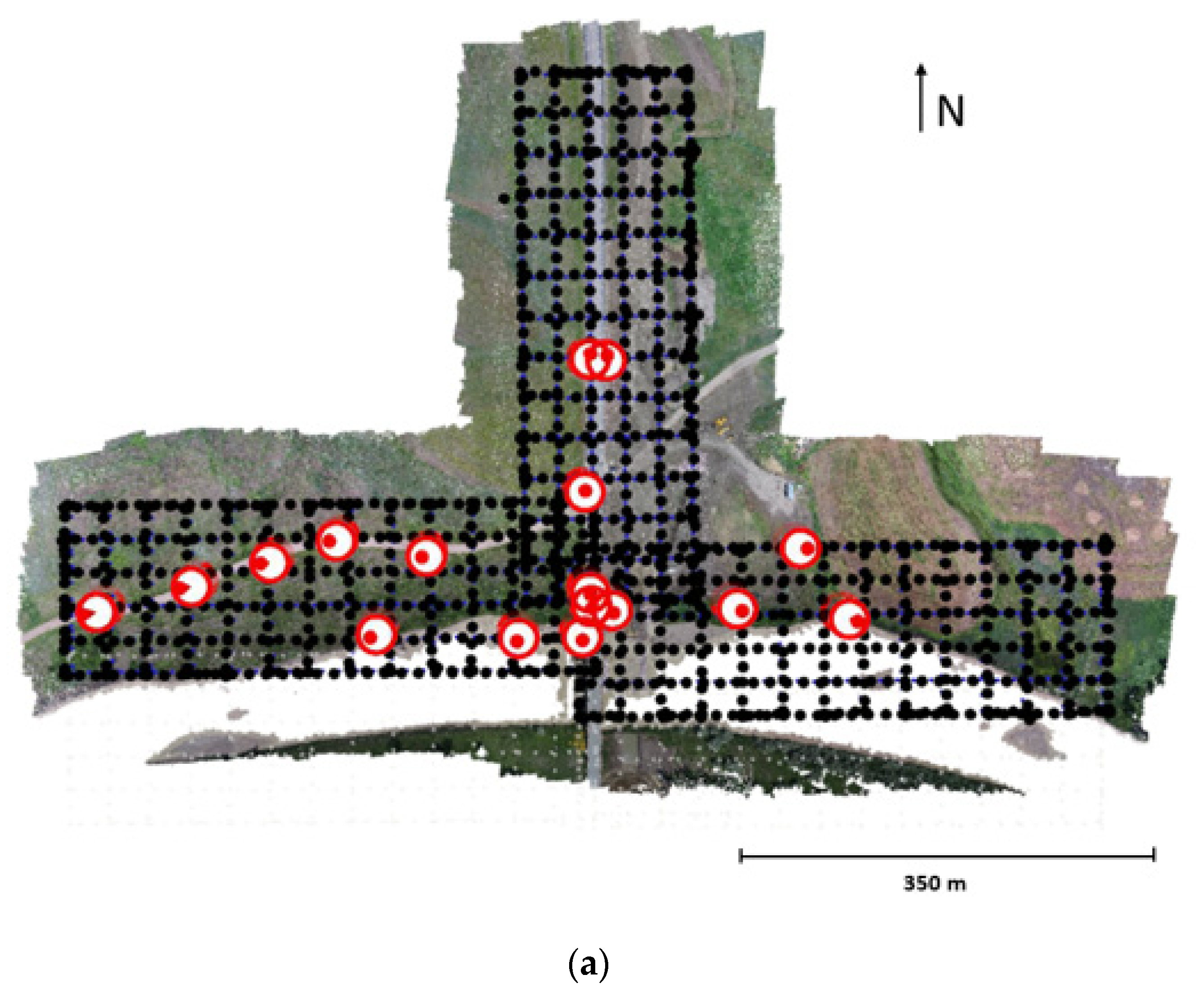
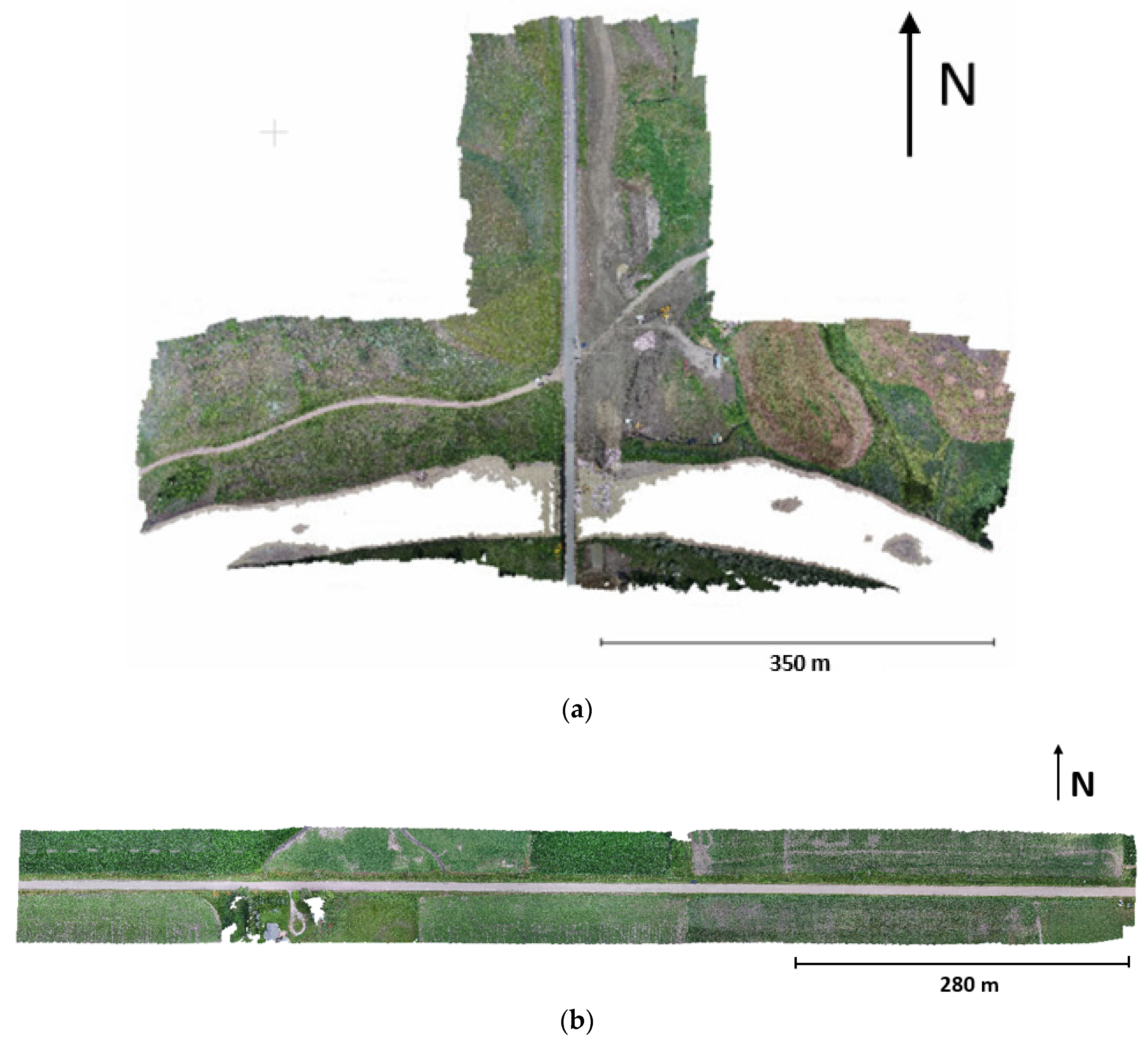
1.3. Description of the Two Sites
2. Methodology
2.1. Data Collection
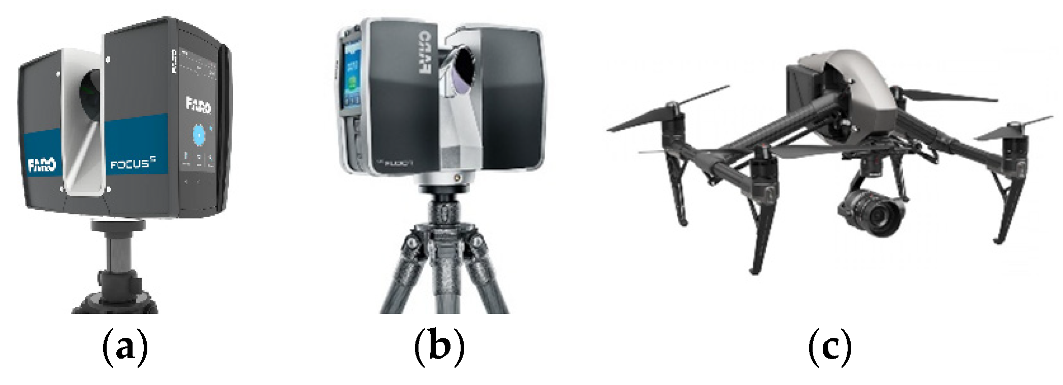
2.1.1. UAS
2.1.2. Real-Time Kinematic Ground Control Survey
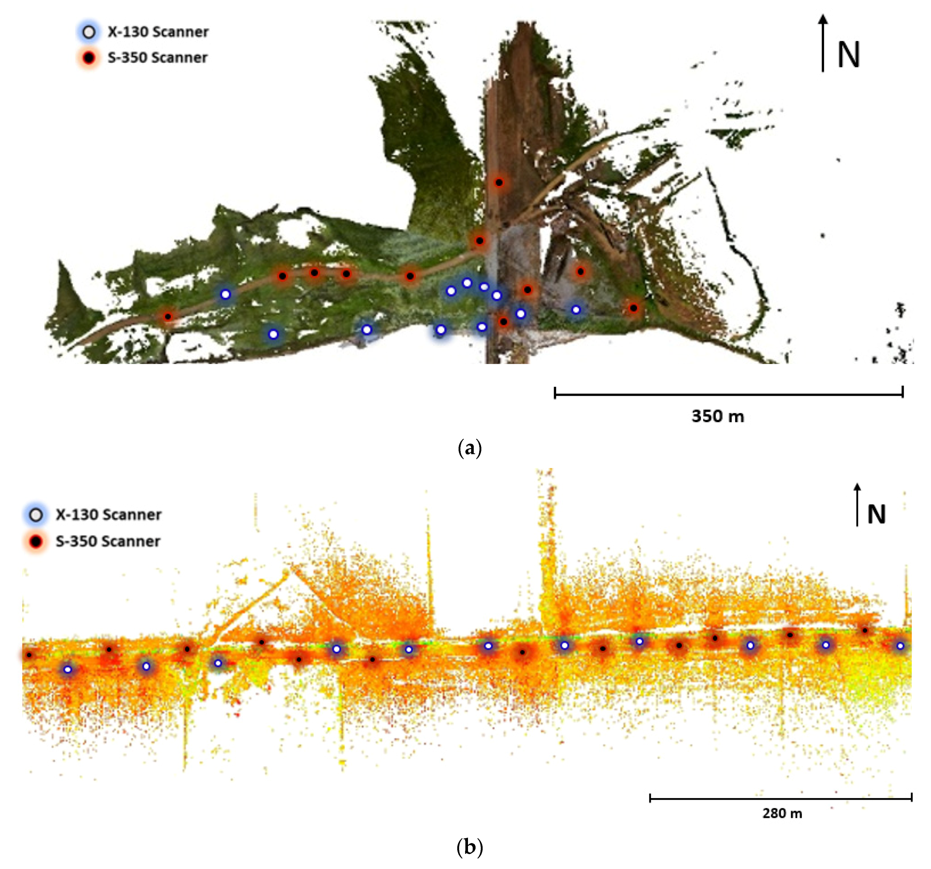
2.1.3. Lidar
2.2. Data Processing
3. Results
3.1. Viewpoint Quality Assessment and Control of the Point Clouds
3.2. Data Processing
3.2.1. Overview
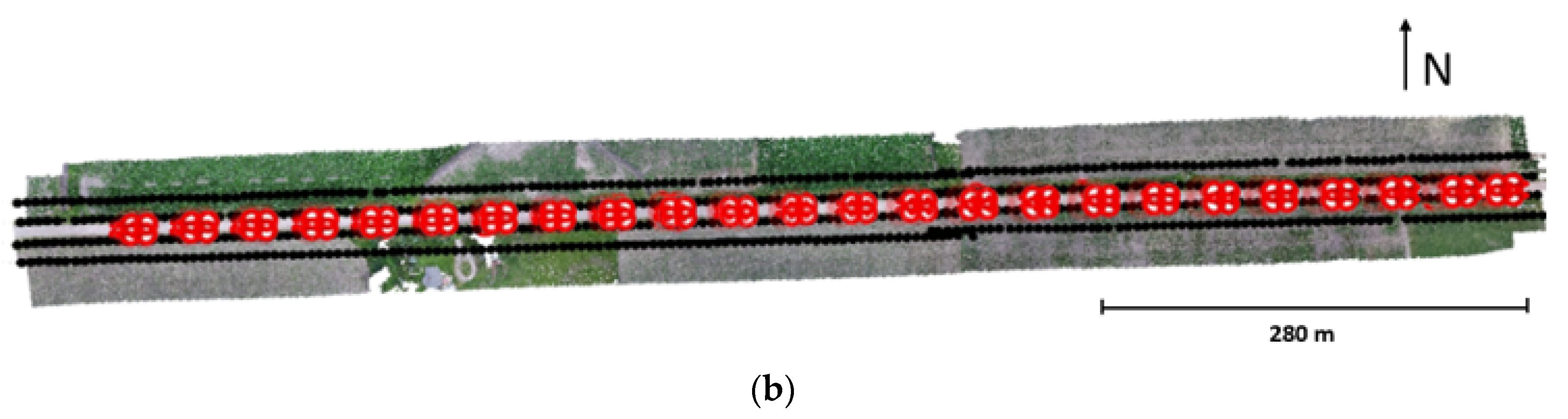
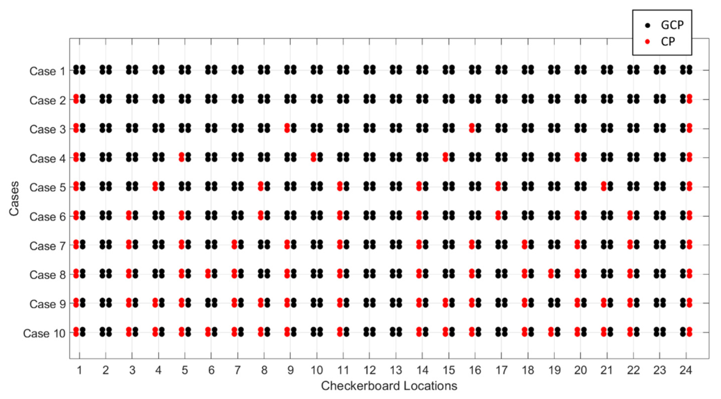
3.2.2. Georeferencing Strategy Comparison
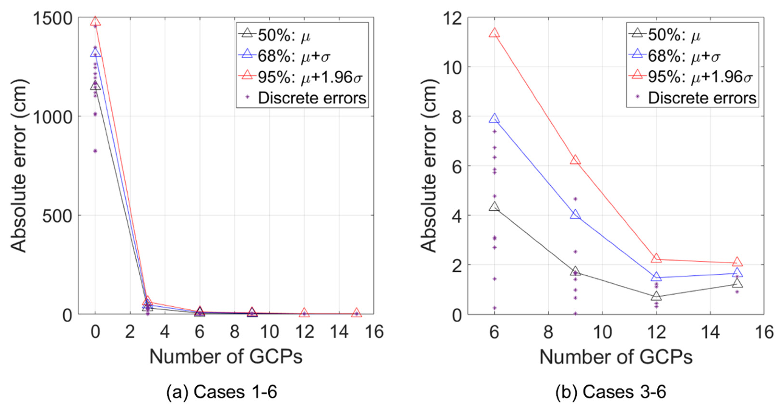
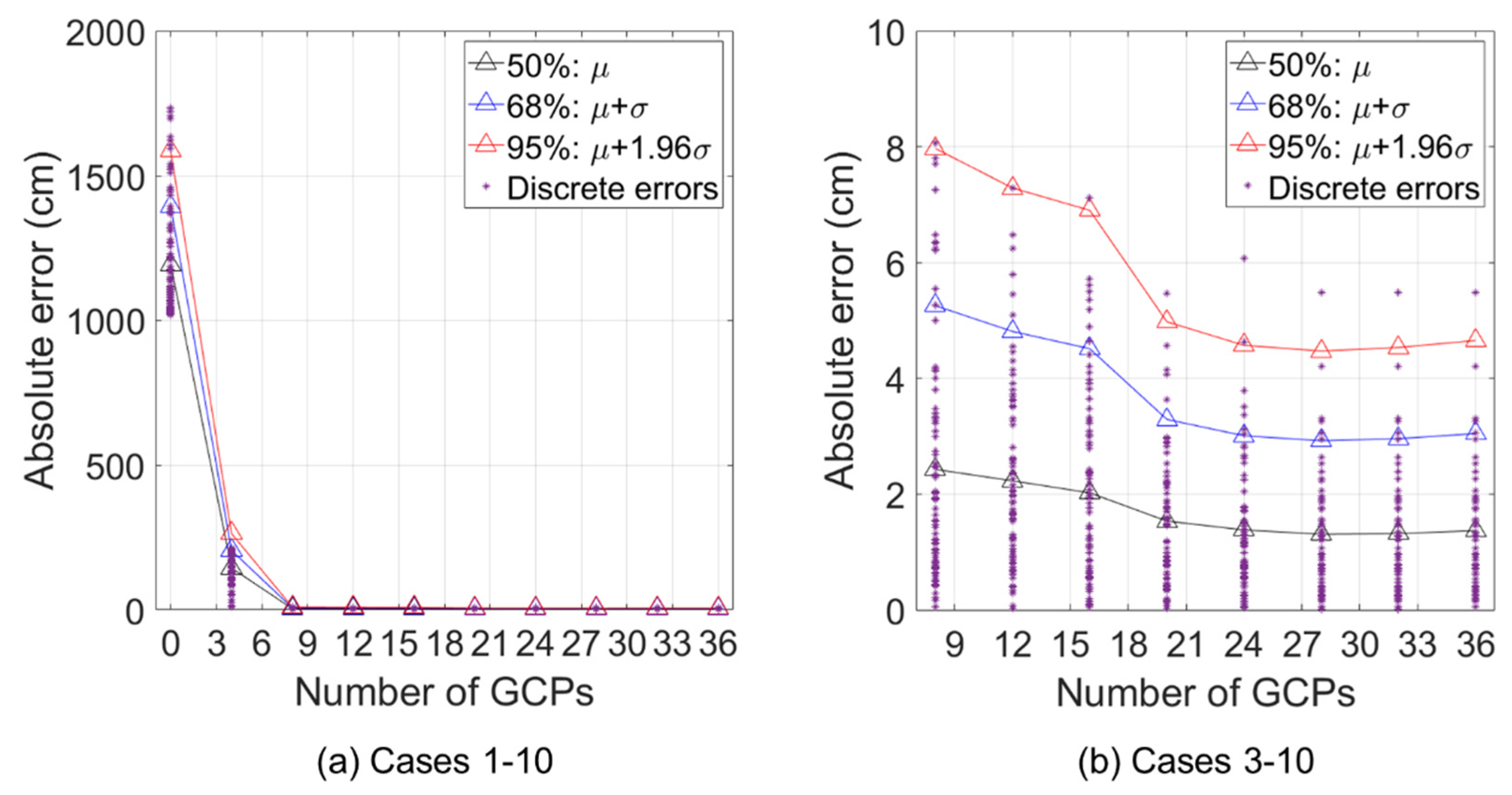
3.2.3. Discrete Errors at Checkpoint (CP) Locations
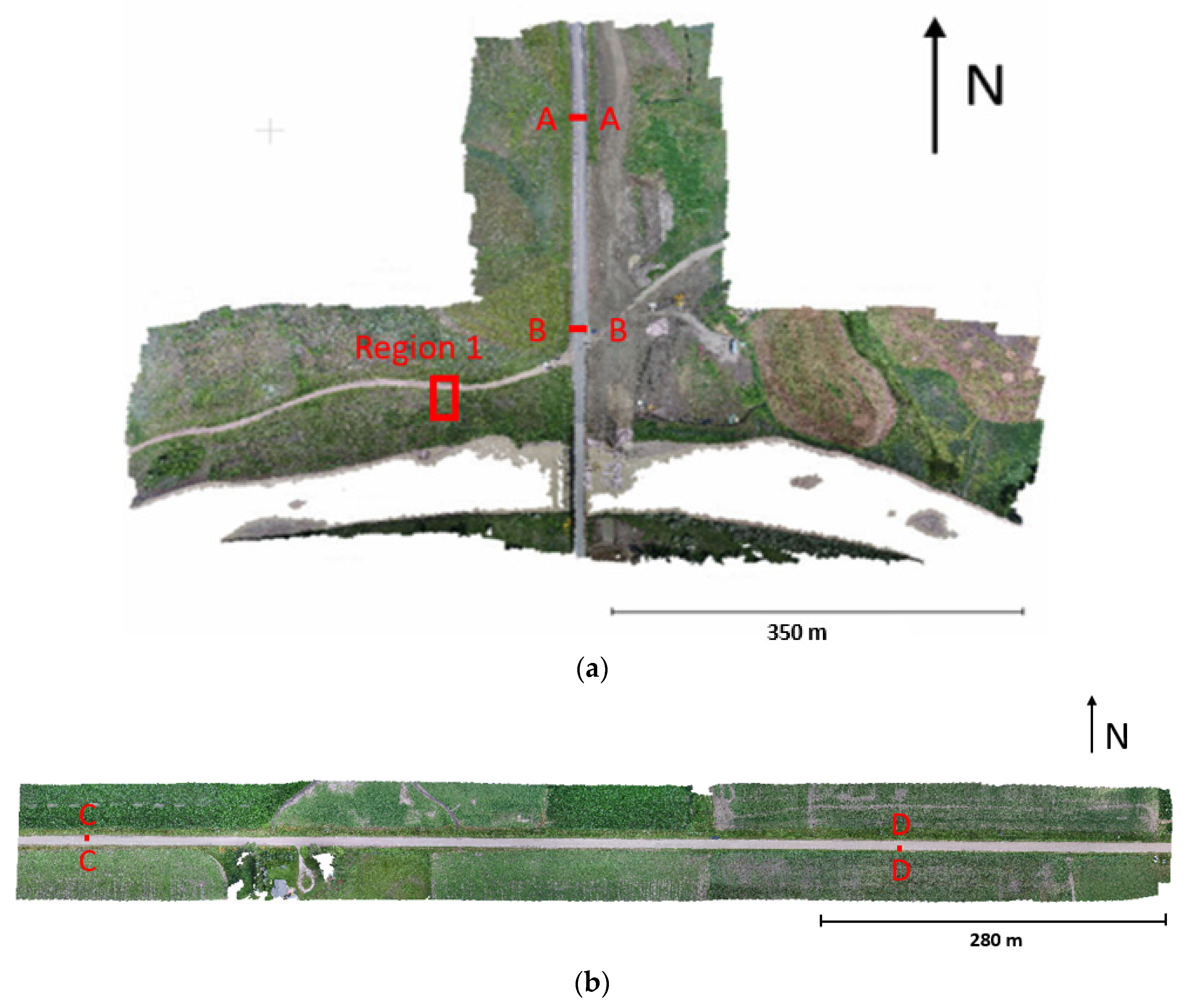
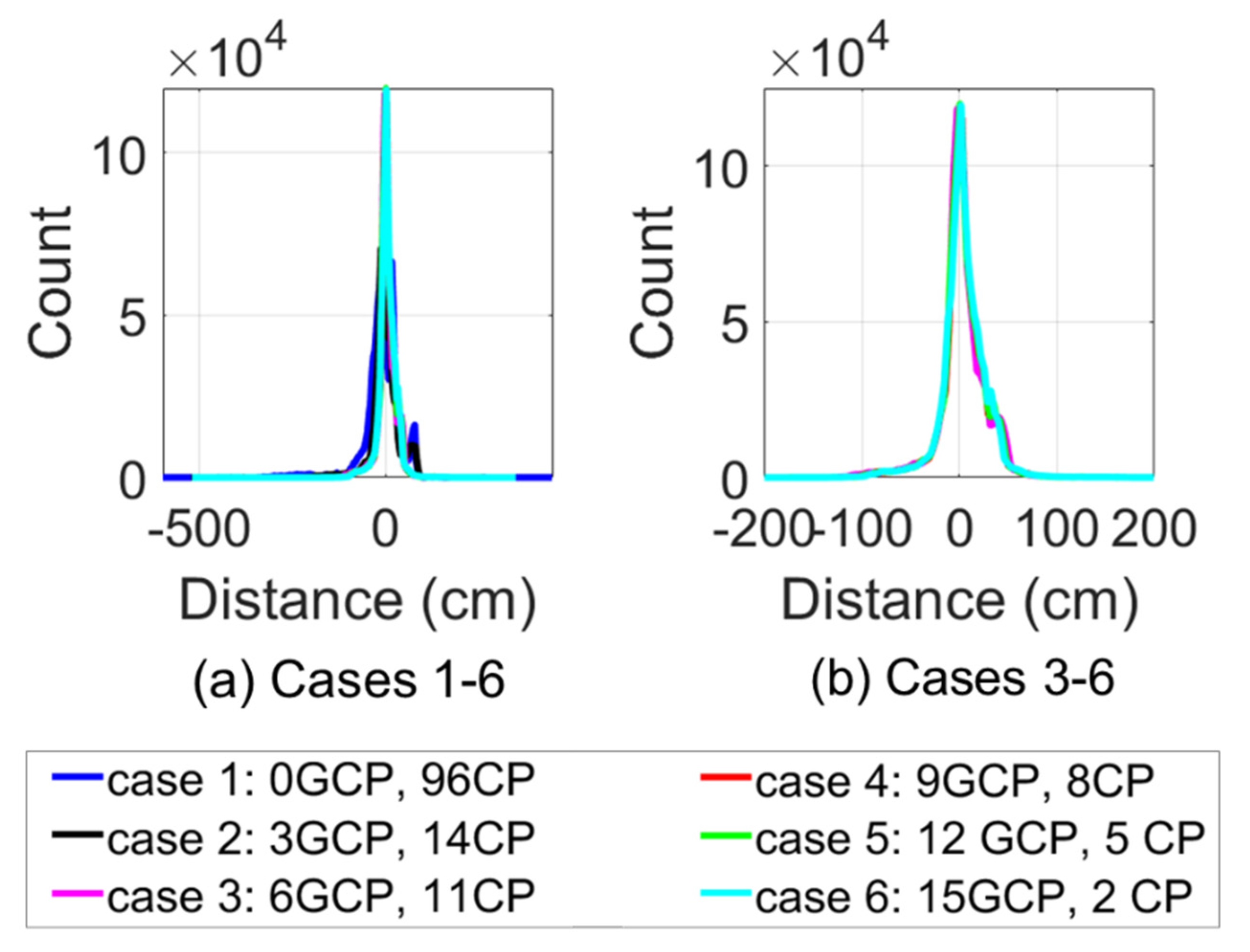
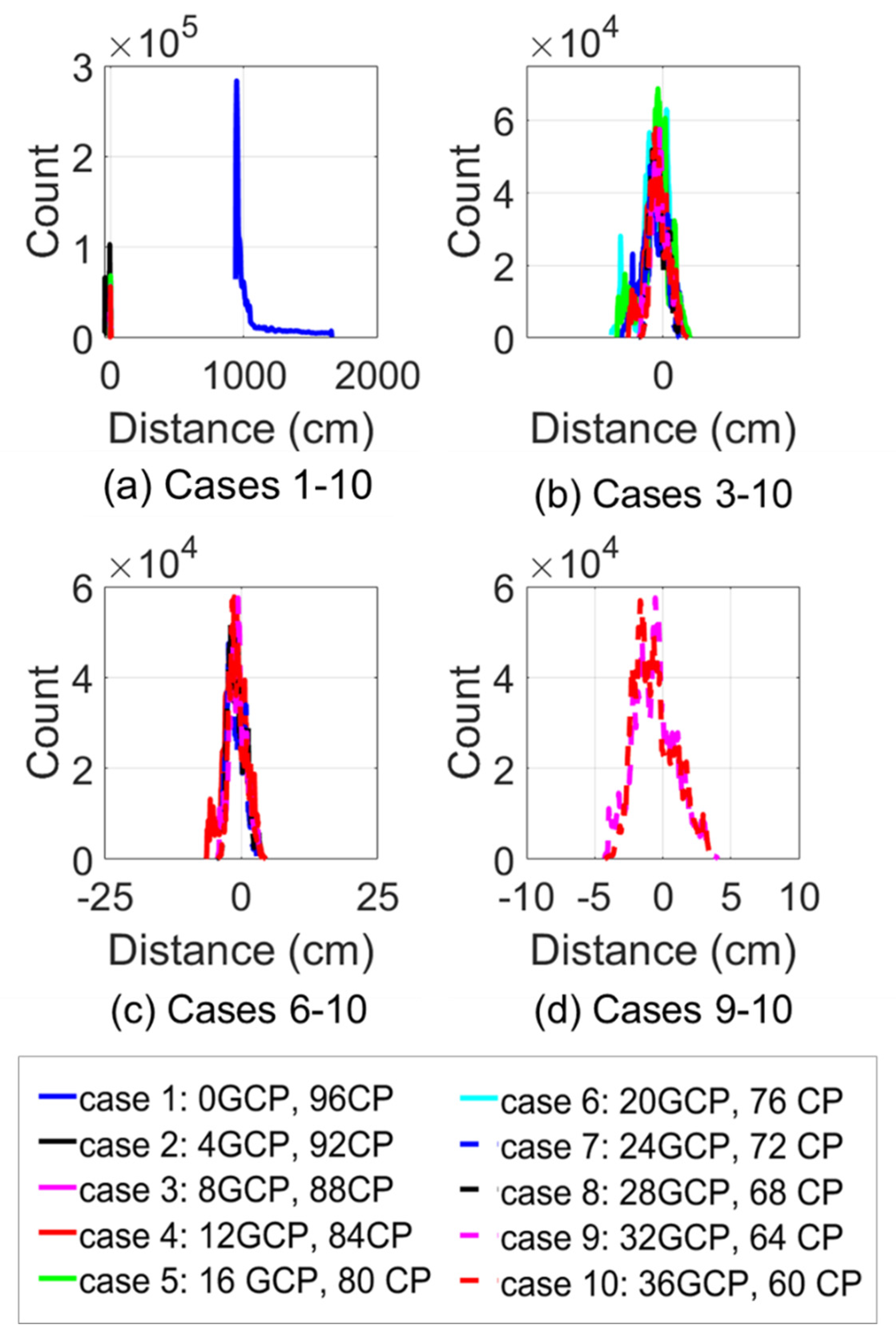
3.2.4. Distributed Errors
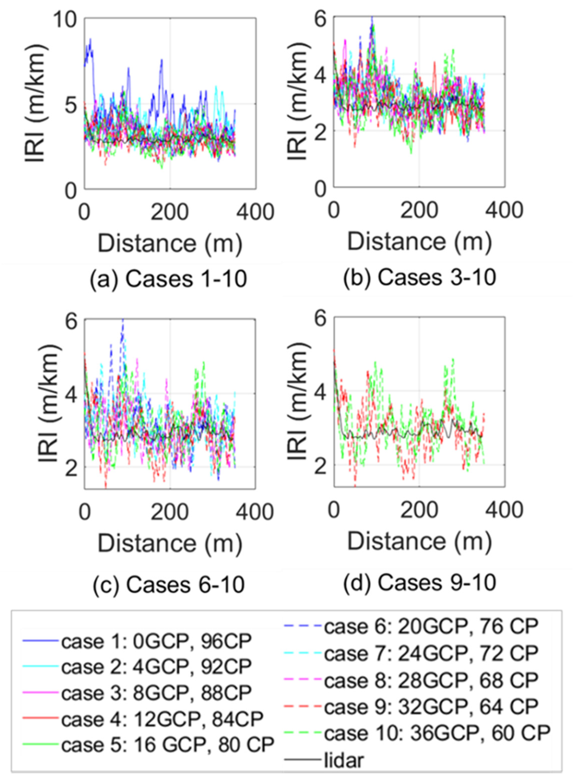
3.2.5. IRI Assessment
4. Discussion
5. Conclusions
Author Contributions
Funding
Acknowledgments
Conflicts of Interest
References
- Liao, Y.; Wood, R.L.; Mohammadi, M.E.; Hughes, P.J.; Womble, J.A. Investigation of Rapid Remote Sensing Techniques for Forensic Wind Analyses, 5th ed.; American Association for Wind Engineering Workshop: Miami, FL, USA, 2018. [Google Scholar]
- Olsen, M.J. In Situ Change Analysis and Monitoring through Terrestrial Laser Scanning. J. Comput. Civ. Eng. 2015, 29, 4014040. [Google Scholar] [CrossRef]
- Dunham, L.; Wartman, J.; Olsen, M.J.; O’Banion, M.; Cunningham, K. Rockfall Activity Index (RAI): A lidar-derived, morphology-based method for hazard assessment. Eng. Geol. 2017, 221, 184–192. [Google Scholar] [CrossRef]
- Ellis, S.A. Using mobile lidar to deliver survey accurate data. In Proceedings of the Transportation Research Board 96th Annual Meeting, TRB, Washington, DC, USA, 8–12 January 2017; p. 17-00597. [Google Scholar]
- Galarreta, J.F.; Kerle, N.; Gerke, M. UAV-based urban structural damage assessment using object-based image analysis and semantic reasoning. Nat. Hazards Earth Syst. Sci. Discuss. 2014, 2, 5603–5645. [Google Scholar] [CrossRef]
- Federal Aviation Agency (FAA). Fact Sheet—Small Unmanned Aircraft Regulations (Part 107). 2016. Available online: https://www.faa.gov/news/fact_sheets/news_story.cfm?newsId=22615 (accessed on 6 October 2020).
- Wood, R.L.; Mohammadi, M.E. Lidar scanning with supplementary UAV captured Images for structural inspections. In Proceedings of the International LiDAR Mapping Forum 2015, Denver, CO, USA, 23–25 February 2015. [Google Scholar]
- Gargoum, S.; El-Basyouny, K.; Sabbagh, J.; Froese, K. Automated Highway Sign Extraction Using Lidar Data. Transp. Res. Rec. J. Transp. Res. Board 2017, 2643, 1–8. [Google Scholar] [CrossRef]
- Eker, R.; Aydın, A.; Hübl, J. Unmanned aerial vehicle (UAV)-based monitoring of a landslide: Gallenzerkogel landslide (Ybbs-Lower Austria) case study. Environ. Monit. Assess. 2017, 190, 28. [Google Scholar] [CrossRef] [PubMed]
- Federal Highway Administration (FHWA). Guide for Efficient Geospatial Data Acquisition Using Lidar Surveying Technology; Rep. No. FHWA-HIF-16-010; FHWA: Washington, DC, USA, 2016.
- Olsen, M.J.; Kayen, R.E. Post-Earthquake and Tsunami 3D Laser Scanning Forensic Investigations. Forensic Eng. 2012 2012, 477–486. [Google Scholar] [CrossRef]
- Yu, H.; Mohammed, M.A.; Mohammadi, M.E.; Moaveni, B.; Barbosa, A.R.; Stavridis, A.; Wood, R.L. Structural Identification of an 18-Story RC Building in Nepal Using Post-Earthquake Ambient Vibration and Lidar Data. Front. Built Environ. 2017, 3, 11. [Google Scholar] [CrossRef]
- Van Oldenborgh, G.J.; van der Wiel, K.; Sebastian, A.; Singh, R.; Arrighi, J.; Otto, F.; Haustein, K.; Li, S.; Vecchi, G.; Cullen, H.M. Attribution of extreme rainfall from Hurricane Harvey, August 2017. Environ. Res. Lett. 2017, 12, 12. [Google Scholar]
- Kijewski-Correa, T.; Gong, J.; Womble, A.; Kennedy, A.; Cai, S.C.S.; Cleary, J.; Dao, T.; Leite, F.; Liang, D.; Peterman, K.; et al. Hurricane Harvey (Texas) Supplement-Collaborative Research: Geotechnical Extreme Events Reconnaissance (GEER) Association: Turning Disaster into Knowledge, DesignSafe-CI, 2018. Dataset 2008. [Google Scholar] [CrossRef]
- Zhou, Z.; Gong, J.; Guo, M. Image-Based 3D Reconstruction for Posthurricane Residential Building Damage Assessment. J. Comput. Civ. Eng. 2016, 30, 4015015. [Google Scholar] [CrossRef]
- Adams, S.M.; Levitan, M.L.; Friedland, C.J.; Jones, C.P.; Griffis, L.G. High Resolution Imagery Collection Utilizing Unmanned Aerial Vehicles (UAVs) for Post-Disaster Studies. Adv. Hurric. Eng. 2012, 777–793. [Google Scholar] [CrossRef]
- Chiu, W.; Ong, W.; Kuen, T.; Courtney, F. Large Structures Monitoring Using Unmanned Aerial Vehicles. Procedia Eng. 2017, 188, 415–423. [Google Scholar] [CrossRef]
- Wing, M.G.; Eklund, A.; Kellogg, L.D. Consumer-Grade Global Positioning System (GPS) Accuracy and Reliability. J. For. 2005, 103, 169–173. [Google Scholar] [CrossRef]
- Nesbit, P.; Hugenholtz, C.H. Enhancing UAV–SfM 3D Model Accuracy in High-Relief Landscapes by Incorporating Oblique Images. Remote Sens. 2019, 11, 239. [Google Scholar] [CrossRef]
- Zang, Y.; Yang, B.; Li, J.; Guan, H. An Accurate TLS and UAV Image Point Clouds Registration Method for Deformation Detection of Chaotic Hillside Areas. Remote Sens. 2019, 11, 647. [Google Scholar] [CrossRef]
- Langhammer, J.; Janský, B.; Kocum, J.; Minařík, R. 3-D reconstruction of an abandoned montane reservoir using UAV photogrammetry, aerial LiDAR and field survey. Appl. Geogr. 2018, 98, 9–21. [Google Scholar] [CrossRef]
- Chandler, J.H.; Buckley, S. Structure from motion (SFM) photogrammetry vs terrestrial laser scanning. In Geoscience Handbook, 5th ed.; AGI Data Sheets; American Geosciences Institute: Alexandria, VA, USA, 2016; Section 20.1. [Google Scholar]
- Ouédraogo, M.M.; Degré, A.; Debouche, C.; Lisein, J. The evaluation of unmanned aerial system-based photogrammetry and terrestrial laser scanning to generate DEMs of agricultural watersheds. Geomorphology 2014, 214, 339–355. [Google Scholar] [CrossRef]
- Thiebes, B.; Tomelleri, E.; Mejia-Aguilar, A.; Rabanser, M.; Schlögel, R.; Mulas, M.; Corsini, A. Assessment of the 2006 to 2015 Corvara landslide evolution using a UAV-derived DSM and orthophoto. Landslides Eng. Slopes Exp. Theory Pract. 2016, 1897–1902. [Google Scholar] [CrossRef]
- Dobson, R.J.; Brooks, C.; Roussi, C.; Colling, T.; Brooks, C.L. Developing an unpaved road assessment system for practical deployment with high-resolution optical data collection using a helicopter UAV. In Proceedings of the 2013 International Conference on Unmanned Aircraft Systems (ICUAS), Atlanta, GA, USA, 28–31 May 2013. [Google Scholar]
- Zhang, C.; Elaksher, A. An Unmanned Aerial Vehicle-Based Imaging System for 3D Measurement of Unpaved Road Surface Distresses1. Comput. Civ. Infrastruct. Eng. 2011, 27, 118–129. [Google Scholar] [CrossRef]
- Liao, Y.; Mohammadi, M.E.; Wood, R.L.; Kim, Y.R. Improvement of Low Traffic Volume Gravel Roads in Nebraska (No. SPR-P1 (16) M040); Nebraska Department of Transportation: Lincoln, NE, USA, 2020.
- Jenkins, M.D.; Buggy, T.; Morison, G. An imaging system for visual inspection and structural condition monitoring of railway tunnels. In Proceedings of the 2017 IEEE Workshop, Environmental Energy and Structural Monitoring Systems, Milan, Italy, 24–25 July 2017; IEEE: Piscataway, NJ, USA, 2017; pp. 1–6. [Google Scholar]
- Soni, A.; Robson, S.; Gleeson, B. Structural monitoring for the rail industry using conventional survey, laser scanning and photogrammetry. Appl. Geomat. 2015, 7, 123–138. [Google Scholar] [CrossRef]
- Markiewicz, J.; Łapiński, S.; Kot, P.; Tobiasz, A.; Muradov, M.; Nikel, J.; Shaw, A.; Al-Shamma’A, A. The Quality Assessment of Different Geolocalisation Methods for a Sensor System to Monitor Structural Health of Monumental Objects. Sensors 2020, 20, 2915. [Google Scholar] [CrossRef] [PubMed]
- O’Banion, M.S.; Olsen, M.J.; Rault, C.; Wartman, J.; Cunningham, K. Suitability of structure from motion for rock-slope assessment. Photogramm. Rec. 2018, 33, 217–242. [Google Scholar] [CrossRef]
- Wu, H.; Zheng, D.; Zhang, Y.-J.; Li, D.-Y.; Nian, T.-K. A photogrammetric method for laboratory-scale investigation on 3D landslide dam topography. Bull. Int. Assoc. Eng. Geol. 2020, 1–16. [Google Scholar] [CrossRef]
- Hasheminasab, S.M.; Zhou, T.; Habib, A. GNSS/INS-Assisted Structure from Motion Strategies for UAV-Based Imagery over Mechanized Agricultural Fields. Remote Sens. 2020, 12, 351. [Google Scholar] [CrossRef]
- Arriola-Valverde, S.; Villagra-Mendoza, K.; Mendez-Morales, M.; Solorzano-Quintana, M.; Gomez-Calderon, N.; Rimolo-Donadio, R. Analysis of Crop Dynamics through Close-Range UAS Photogrammetry. In Proceedings of the 2020 IEEE International Symposium on Circuits and Systems (ISCAS), Sevilla, Spain, 10–21 October 2020; Institute of Electrical and Electronics Engineers (IEEE): Piscataway, NJ, USA, 2020; pp. 1–5. [Google Scholar]
- Gil-Docampo, M.; Arza-García, M.; Ortiz-Sanz, J.; Martínez-Rodríguez, S.; Marcos-Robles, J.L.; Sánchez-Sastre, L.F. Above-ground biomass estimation of arable crops using UAV-based SfM photogrammetry. Geocarto Int. 2019, 35, 687–699. [Google Scholar] [CrossRef]
- Liao, Y.; Mohammadi, M.E.; Wood, R.L. Deep Learning Classification of 2D Orthomosaic Images and 3D Point Clouds for Post-Event Structural Damage Assessment. Drones 2020, 4, 24. [Google Scholar] [CrossRef]
- Saovana, N.; Yabuki, N.; Fukuda, T. Development of an unwanted-feature removal system for Structure from Motion of repetitive infrastructure piers using deep learning. Adv. Eng. Inform. 2020, 46, 101169. [Google Scholar] [CrossRef]
- Lague, D.; Brodu, N.; Leroux, J. Accurate 3D comparison of complex topography with terrestrial laser scanner: Application to the Rangitikei canyon (N-Z). ISPRS J. Photogramm. Remote Sens. 2013, 82, 10–26. [Google Scholar] [CrossRef]
- Warrick, J.A.; Ritchie, A.C.; Schmidt, K.M.; Reid, M.E.; Logan, J. Characterizing the catastrophic 2017 Mud Creek landslide, California, using repeat structure-from-motion (SfM) photogrammetry. Landslides 2019, 16, 1201–1219. [Google Scholar] [CrossRef]
- Peppa, M.V.; Mills, J.P.; Moore, P.; Miller, P.E.; Chambers, J.E. Automated co-registration and calibration in SfM photogrammetry for landslide change detection. Earth Surf. Process. Landf. 2018, 44, 287–303. [Google Scholar] [CrossRef]
- Rossi, P.; Castagnetti, C.; Capra, A.; Brooks, A.J.; Mancini, F. Detecting change in coral reef 3D structure using underwater photogrammetry: Critical issues and performance metrics. Appl. Geomat. 2019, 12, 3–17. [Google Scholar] [CrossRef]
- Cawood, F.; Yu, M.; Kolapo, P.; Qin, C. Development of a Laboratory for Testing the Accuracy of Terrestrial 3D Laser Scanning Technologies. Int. J. Georesources Environ. 2018, 4, 105–114. [Google Scholar] [CrossRef]
- Guisado-Pintado, E.; Jackson, D.W.; Rogers, D. 3D mapping efficacy of a drone and terrestrial laser scanner over a temperate beach-dune zone. Geomorphology 2019, 328, 157–172. [Google Scholar] [CrossRef]
- Nouwakpo, S.K.; Weltz, M.A.; McGwire, K. Assessing the performance of structure-from-motion photogrammetry and terrestrial LiDAR for reconstructing soil surface microtopography of naturally vegetated plots. Earth Surf. Process. Landf. 2015, 41, 308–322. [Google Scholar] [CrossRef]
- Zaragoza, I.M.-E.; Caroti, G.; Piemonte, A.; Riedel, B.; Tengen, D.; Niemeier, W. Structure from motion (SfM) processing of UAV images and combination with terrestrial laser scanning, applied for a 3D-documentation in a hazardous situation. Geomat. Nat. Hazards Risk 2017, 8, 1492–1504. [Google Scholar] [CrossRef]
- Zhou, Y.; Rupnik, E.; Faure, P.-H.; Pierrot-Deseilligny, M. GNSS-Assisted Integrated Sensor Orientation with Sensor Pre-Calibration for Accurate Corridor Mapping. Sensors 2018, 18, 2783. [Google Scholar] [CrossRef] [PubMed]
- Womble, J.A.; Wood, R.L.; Smith, D.A.; Louden, E.I.; Mohammadi, M.E.; Soules, J.G. (Greg). Reality Capture for Tornado Damage to Structures. In Proceedings of the Structures Congress 2017, Denver, CO, USA, 6–8 April 2017. [Google Scholar]
- Graham, L. Drone mapping—SfM versus low precision lidar. In GeoCue; GeoCue Group: Madison, AL, USA, 19 June 2018. [Google Scholar]
- Fonstad, M.A.; Dietrich, J.T.; Courville, B.C.; Jensen, J.L.; Carbonneau, P.E. Topographic structure from motion: A new development in photogrammetric measurement. Earth Surf. Process. Landf. 2013, 38, 421–430. [Google Scholar] [CrossRef]
- Sayers, M.W. On the calculation of international roughness index from longitudinal road profile. Transp. Res. Rec. 1995, 1501, 1–12. [Google Scholar]
- Alhasan, A.A.; Younkin, K.; White, D.J. Comparison of Roadway Roughness Derived from LIDAR and SFM 3D Point Clouds. Trans Proj. Rep. 2015. [Google Scholar]
- Zak, J. On laser scanning, pavement surface roughness and international roughness index in highway construction. In Proceedings of the 6th Eurasphalt & Eurobitume Congress, Prague, Czech Republic, 1–3 June 2016. [Google Scholar]
- Tonkin, T.N.; Midgley, N.G. Ground-Control Networks for Image Based Surface Reconstruction: An Investigation of Optimum Survey Designs Using UAV Derived Imagery and Structure-from-Motion Photogrammetry. Remote Sens. 2016, 8, 786. [Google Scholar] [CrossRef]
- Tahar, K.N. An Evaluation on Different Number of Ground Control Points in Unmanned Aerial Vehicle Photogrammetric Block. ISPRS Int. Arch. Photogramm. Remote Sens. Spat. Inf. Sci. 2013, 40, 93–98. [Google Scholar] [CrossRef]
- Javernick, L.; Brasington, J.; Caruso, B. Modeling the topography of shallow braided rivers using Structure-from-Motion photogrammetry. Geomorphology 2014, 213, 166–182. [Google Scholar] [CrossRef]
- Agüera-Vega, F.; Carvajal-Ramírez, F.; Martínez-Carricondo, P. Assessment of photogrammetric mapping accuracy based on variation ground control points number using unmanned aerial vehicle. Measurement 2017, 98, 221–227. [Google Scholar] [CrossRef]
- Caroti, G.; Zaragoza, I.M.-E.; Piemonte, A. Accuracy Assessment in Structure from Motion 3d Reconstruction from Uav-Born Images: The Influence of the Data Processing Methods. ISPRS Int. Arch. Photogramm. Remote. Sens. Spat. Inf. Sci. 2015, 103–109. [Google Scholar] [CrossRef]
- Gindraux, S.; Boesch, R.; Farinotti, D. Accuracy Assessment of Digital Surface Models from Unmanned Aerial Vehicles’ Imagery on Glaciers. Remote Sens. 2017, 9, 186. [Google Scholar] [CrossRef]
- Agüera-Vega, F.; Carvajal-Ramírez, F.; Martínez-Carricondo, P. Accuracy of Digital Surface Models and Orthophotos Derived from Unmanned Aerial Vehicle Photogrammetry. J. Surv. Eng. 2017, 143, 4016025. [Google Scholar] [CrossRef]
- FARO. FARO Laser Scanner Focus 3D: Features, Benefits & Technical Specifications; FARO Technologies: Lake Mary, FL, USA, 2011. [Google Scholar]
- Jaboyedoff, M.; Oppikofer, T.; Abellán, A.; Derron, M.-H.; Loye, A.; Metzger, R.; Pedrazzini, A. Use of LIDAR in landslide investigations: A review. Nat. Hazards 2010, 61, 5–28. [Google Scholar] [CrossRef]
- Fowler, A.; Kadatskiy, V. Accuracy and error assessment of terrestrial, mobile and airborne lidar. In Proceedings of the American Society of Photogrammetry and Remote Sensing Conference (ASPRP 2011), Milwaukee, WI, USA, 1–5 May 2011. [Google Scholar]
- James, M.R.; Robson, S. Straightforward reconstruction of 3D surfaces and topography with a camera: Accuracy and geoscience application. J. Geophys. Res. Space Phys. 2012, 117, 3. [Google Scholar] [CrossRef]
- South Dakota Department of Transportation (SDDOT). Road Design Manual; Chapter 7; Cross Sections. 2019. Available online: http://sddot.com/business/design/docs/rd/rdmch07.pdf (accessed on 1 July 2019).
- Forlani, G.; Dall’Asta, E.; Diotri, F.; Cella, U.M.D.; Roncella, R.; Santise, M. Quality Assessment of DSMs Produced from UAV Flights Georeferenced with On-Board RTK Positioning. Remote Sens. 2018, 10, 311. [Google Scholar] [CrossRef]
- Sanz-Ablanedo, E.; Chandler, J.H.; Rodríguez-Pérez, J.R.; Ordóñez, C. Accuracy of Unmanned Aerial Vehicle (UAV) and SfM Photogrammetry Survey as a Function of the Number and Location of Ground Control Points Used. Remote Sens. 2018, 10, 1606. [Google Scholar] [CrossRef]
- Federal Geographic Data Committee (FGDC). Geospatial Positioning Accuracy Standards Part 3: National Standard for Spatial Data Accuracy; Report No. FGDC-STD-007.3-1998; USGS: Reston, VA, USA, 1998.
- CloudCompare (Version 2.7). Available online: http://www.cloudcompare.org (accessed on 8 August 2016).
- Sayers, M.W. Guidelines for Conducting and Calibrating Road Roughness Measurements; World Bank Technical Paper no. WTP 46; World Bank Group: Washington, DC, USA, 1986. [Google Scholar]
- Zhang, Z.; Gerke, M.; Vosselman, G.; Yang, M.Y. Patch-based Evaluation of Dense Image Matching Quality. arXiv 2018, arXiv:1807.09546. [Google Scholar] [CrossRef]


| Site | Case | Target Count | GCP Count | CP Count | GCP Count to Target Count (%) |
|---|---|---|---|---|---|
| 1 | 1 | 17 | 0 | 17 | 0.0 |
| 1 | 2 | 17 | 3 | 14 | 17.6 |
| 1 | 3 | 17 | 6 | 11 | 35.3 |
| 1 | 4 | 17 | 9 | 8 | 52.9 |
| 1 | 5 | 17 | 12 | 5 | 70.6 |
| 1 | 6 | 17 | 15 | 2 | 88.2 |
| 2 | 1 | 96 | 0 | 96 | 0.0 |
| 2 | 2 | 96 | 4 | 92 | 4.2 |
| 2 | 3 | 96 | 8 | 88 | 8.3 |
| 2 | 4 | 96 | 12 | 84 | 12.5 |
| 2 | 5 | 96 | 16 | 80 | 16.7 |
| 2 | 6 | 96 | 20 | 76 | 20.8 |
| 2 | 7 | 96 | 24 | 72 | 25.0 |
| 2 | 8 | 96 | 28 | 68 | 29.2 |
| 2 | 9 | 96 | 32 | 64 | 33.3 |
| 2 | 10 | 96 | 36 | 60 | 37.5 |
| Section | Average Width (m) | Average Slope (%) | ||
|---|---|---|---|---|
| Lidar | SfM | Lidar | SfM | |
| A-A | 3.65 | 3.67 | 2.4 | 2.7 |
| B-B | 3.66 | 3.67 | 2.2 | 2.4 |
| Section | Calculated Slope (%) | Digital Level Measurement (%) | |
|---|---|---|---|
| Lidar | SfM | ||
| C-C | 4.08 | 4.12 | 4.0 |
| D-D | 3.36 | 3.58 | 3.3 |
| Quantity | Case 1 | Case 2 | Case 3 | Case 4 | Case 5 | Case 6 |
|---|---|---|---|---|---|---|
| Second moment of area (1 × 107 cm4) | 3.59 | 2.74 | 1.84 | 1.80 | 1.79 | 1.82 |
| Mean (cm) | 9.17 | 0.04 | 3.49 | 4.29 | 4.16 | 4.56 |
| Mode (cm) | 11.91 | 11.77 | 1.89 | 2.95 | 1.03 | 1.97 |
| Standard deviation (cm) | 51.27 | 38.50 | 26.60 | 25.68 | 25.42 | 25.45 |
| Error at 95% CI (cm) | 12.56 | 9.43 | 6.52 | 6.29 | 6.23 | 6.23 |
| Quantity | Case 1 | Case 2 | Case 3 | Case 4 | Case 5 | Case 6 | Case 7 | Case 8 | Case 9 | Case 10 |
|---|---|---|---|---|---|---|---|---|---|---|
| Second moment of area (1 × 106 cm4) | 5542.41 | 113.35 | 12.14 | 10.43 | 10.82 | 9.36 | 7.66 | 7.24 | 6.98 | 6.99 |
| Mean (cm) | 1081.14 | 23.03 | 1.49 | 1.10 | 1.18 | 1.103 | 1.01 | 0.77 | 0.60 | 0.58 |
| Mode (cm) | 945.03 | 6.64 | 0.67 | 0.57 | 0.88 | 1.27 | 1.87 | 1.93 | 0.55 | 1.65 |
| Standard deviation (cm) | 188.5 | 13.11 | 2.78 | 2.38 | 2.62 | 1.99 | 1.45 | 1.45 | 1.55 | 1.49 |
| Error at 95% CI (cm) | 46.19 | 3.21 | 0.68 | 0.58 | 0.64 | 0.49 | 0.36 | 0.36 | 0.38 | 0.37 |
| Quantity | Lidar | Case 1 | Case 2 | Case 3 | Case 4 | Case 5 | Case 6 | Case 7 | Case 8 | Case 9 | Case 10 |
|---|---|---|---|---|---|---|---|---|---|---|---|
| Mean (m/km) | 2.94 | 4.41 | 3.72 | 3.20 | 3.16 | 2.96 | 3.21 | 3.24 | 3.02 | 2.94 | 3.10 |
| Median (m/km) | 2.87 | 4.24 | 3.55 | 3.07 | 3.04 | 2.81 | 3.12 | 3.18 | 2.94 | 2.87 | 3.04 |
| Mode (m/km) | 2.56 | 3.72 | 2.45 | 2.54 | 2.51 | 2.16 | 2.57 | 2.65 | 2.05 | 2.20 | 2.31 |
| Standard deviation (m/km) | 0.33 | 1.67 | 1.13 | 1.00 | 0.77 | 1.00 | 0.94 | 0.94 | 0.83 | 0.88 | 0.93 |
Publisher’s Note: MDPI stays neutral with regard to jurisdictional claims in published maps and institutional affiliations. |
© 2020 by the authors. Licensee MDPI, Basel, Switzerland. This article is an open access article distributed under the terms and conditions of the Creative Commons Attribution (CC BY) license (http://creativecommons.org/licenses/by/4.0/).
Share and Cite
Liao, Y.; Wood, R.L. Discrete and Distributed Error Assessment of UAS-SfM Point Clouds of Roadways. Infrastructures 2020, 5, 87. https://doi.org/10.3390/infrastructures5100087
Liao Y, Wood RL. Discrete and Distributed Error Assessment of UAS-SfM Point Clouds of Roadways. Infrastructures. 2020; 5(10):87. https://doi.org/10.3390/infrastructures5100087
Chicago/Turabian StyleLiao, Yijun, and Richard L. Wood. 2020. "Discrete and Distributed Error Assessment of UAS-SfM Point Clouds of Roadways" Infrastructures 5, no. 10: 87. https://doi.org/10.3390/infrastructures5100087
APA StyleLiao, Y., & Wood, R. L. (2020). Discrete and Distributed Error Assessment of UAS-SfM Point Clouds of Roadways. Infrastructures, 5(10), 87. https://doi.org/10.3390/infrastructures5100087