3.2. Durability Performance Assessment Considering Spatial Variability and Correlation
In this section, the initiation time of the corrosion/cracking of a spatially distributed RC structure is considered. Consider a rectangular surface with a size of
. Without loss of generality, assume that
. Subdividing the surface into
n small cells, as the cell size is small enough, the durability scenario within each cell can be represented by that at a single point within the cell. With this, let a Bernoulli variable
represent the state of the
ith cell at time
t for
, which equals one if failure occurs at the
ith cell and zero otherwise. The structural spatial properties such as the concrete cover thickness, chloride diffusion coefficient, and others will affect the sequence
. Similar to Equation (
10), it follows that,
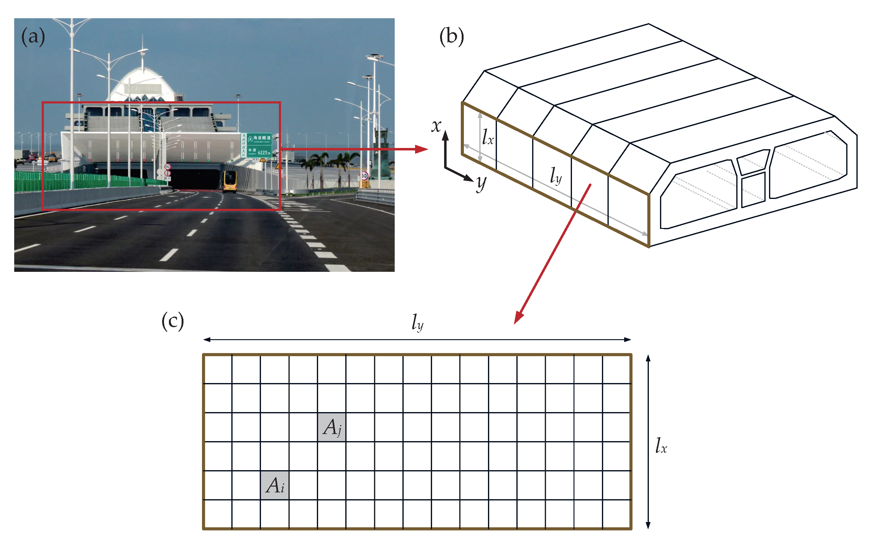
Figure 2 presents an example of the two-dimensional durability problem, which was adopted from the HZM bridge project. Due to common production process and construction practice [
5,
40,
41], the sequence
is spatially correlated (i.e.,
and
are correlated for the
ith and
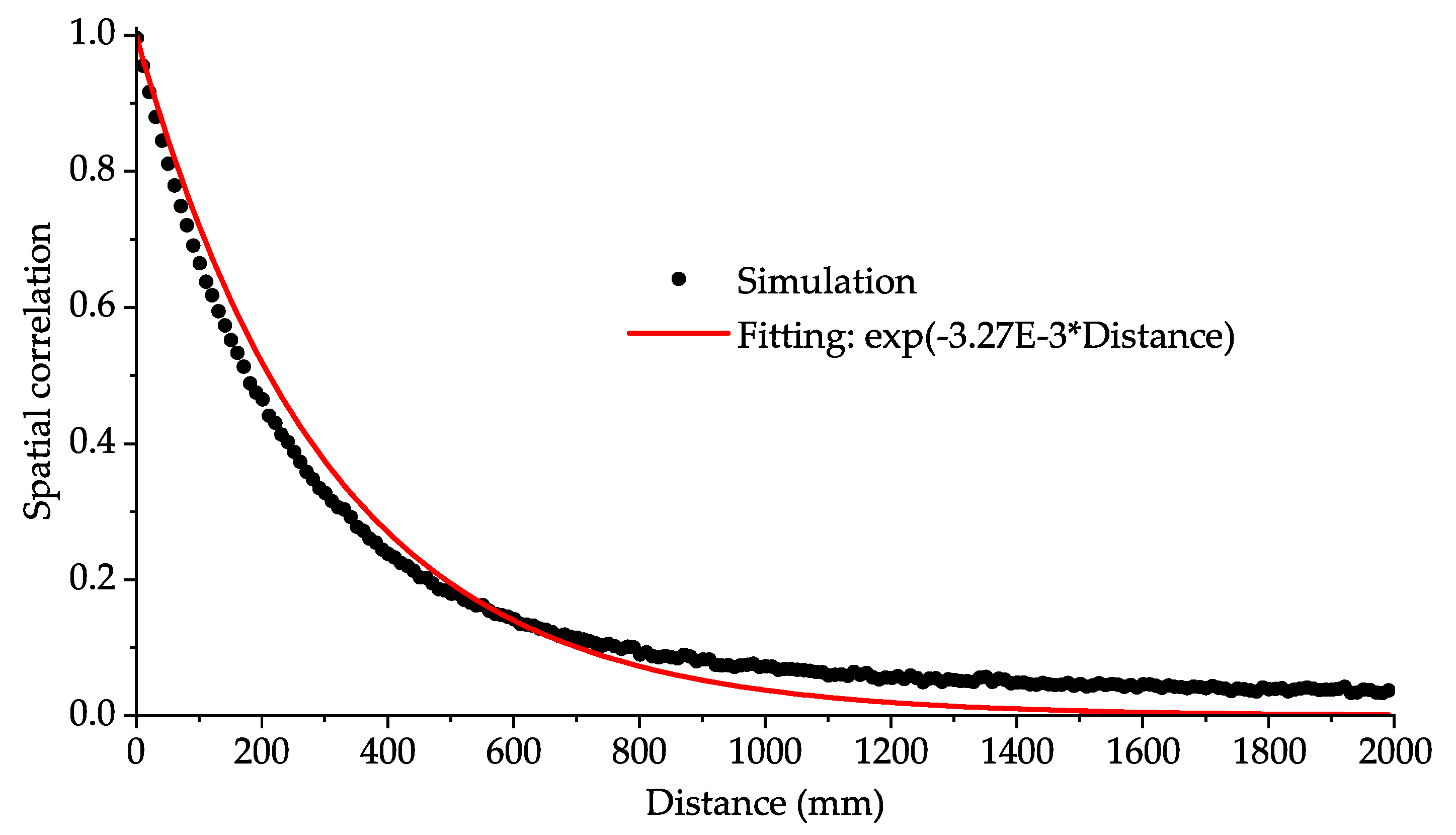
jth cells), and this correlation is expected to be considered in the estimate of surface durability. The correlation function, denoted by
, is a function of the distance of two locations of interest (
ℓ). It by definition equals one when
and decreases with
. Different commonly used models are available in the literature to describe the decay behavior of the spatial correlation. For example, if using the exponential law, it follows that,
in which
is the correlation length, at which the spatial correlation equals
.
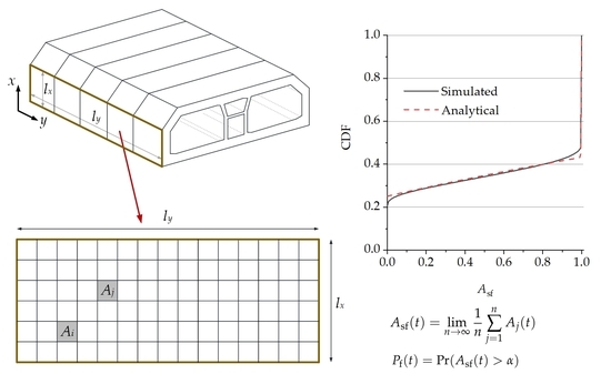
For the whole surface
, the limit state typically no longer focuses on the behavior of a single cell (location) only. In fact, many useful indicators for durability assessment use the proportion of failed concrete surface (e.g., with corrosion/crack initiation). Mathematically, the failure of the surface is defined as the scenario that more than
(
) of the whole area is associated with failed performance. Correspondingly, the limit state function for the whole surface at time
t is given by:
where
is an indicative function, which returns one if the statement in the brackets in true and zero otherwise. Subsequently, according to Equation (
1), the time-dependent failure probability at time
t,
, can be estimated by:
In Equation (
14), while an analytical approach was presented for the estimation of surface failure probability, it is practically difficult to implement since the explicit form of the function
is unknown (which may even take a complicated form). Alternatively, this paper aims to solve Equation (
14) based on the discretization of the surface as in
Figure 2c. In the presence of
n cells as introduced before, let
be the average performance associated with the surface, that is,
With this, Equation (
14) becomes:
If the CDF of
is
, Equation (
16) is rewritten as follows,
and correspondingly, the reliability of the structural surface at time
t is
.
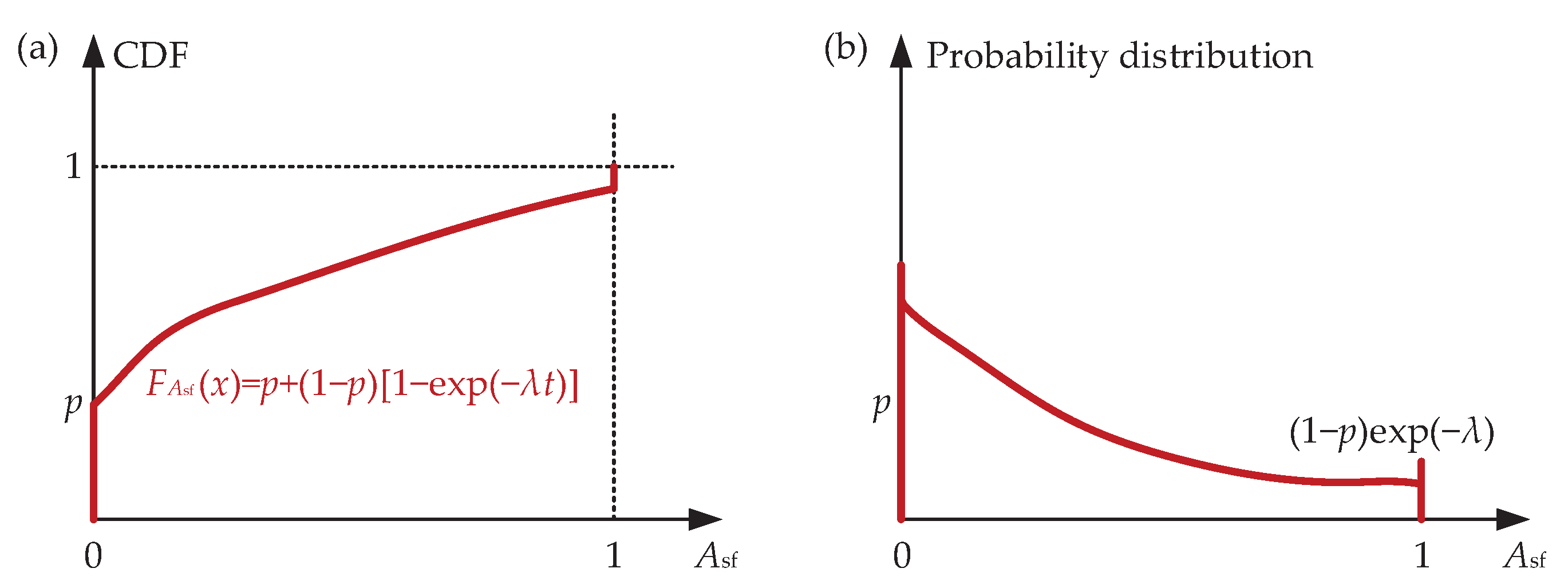
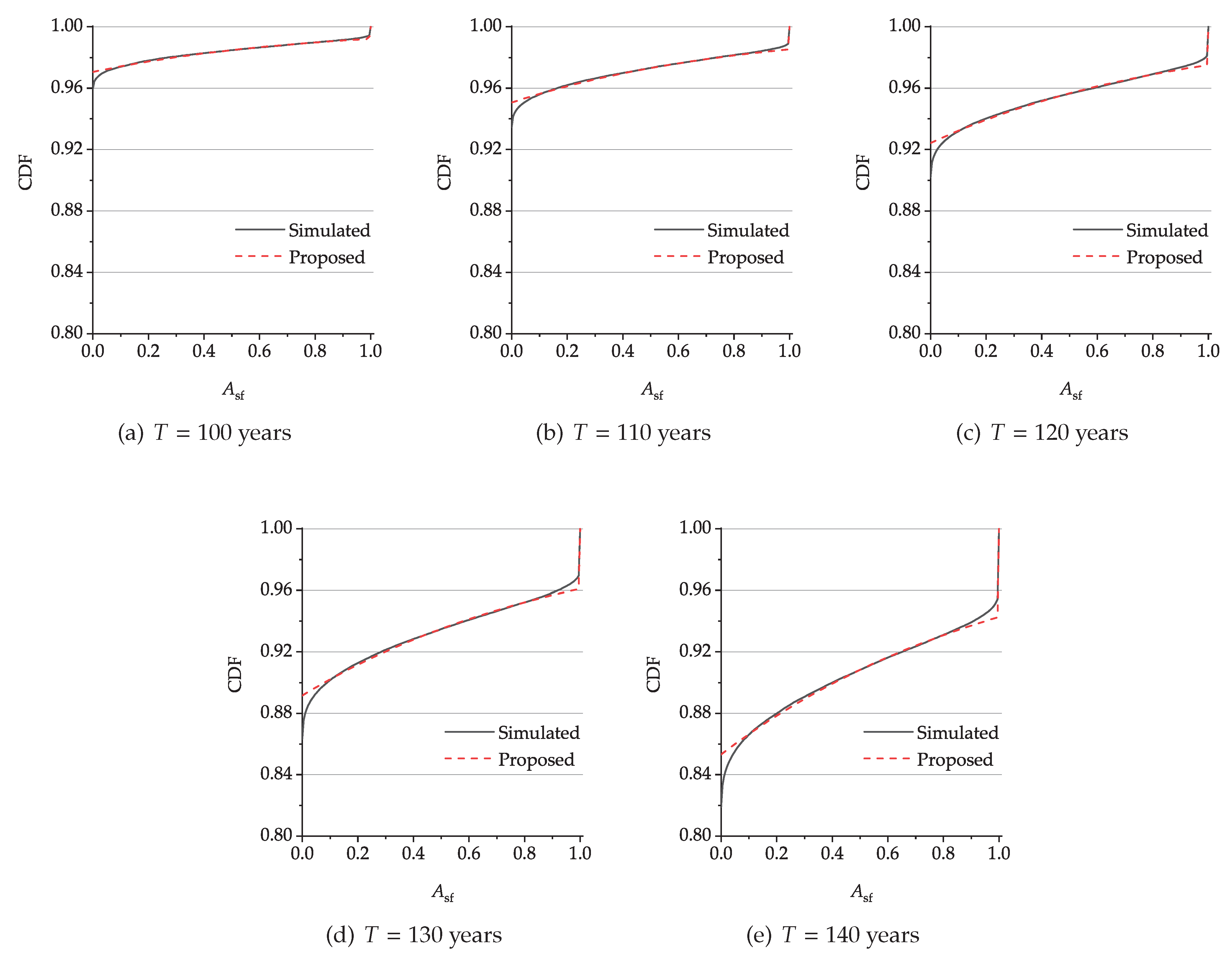
Note that
is strictly defined within the range of
. This paper proposes to use a mixture distribution to model the probabilistic behavior of
, as shown in
Table 1 and
Figure 3. Two parameters are involved, namely
p and
, and will be determined later. In this model, the probability of
equals
p (where
), and the probability of
is
. For the range of
,
is modeled by an exponential distribution with a parameter of
. With such a configuration, the mean value and variance of
are respectively:
and:
in which
and
are the mean value and variance of the variables in the brackets, respectively.
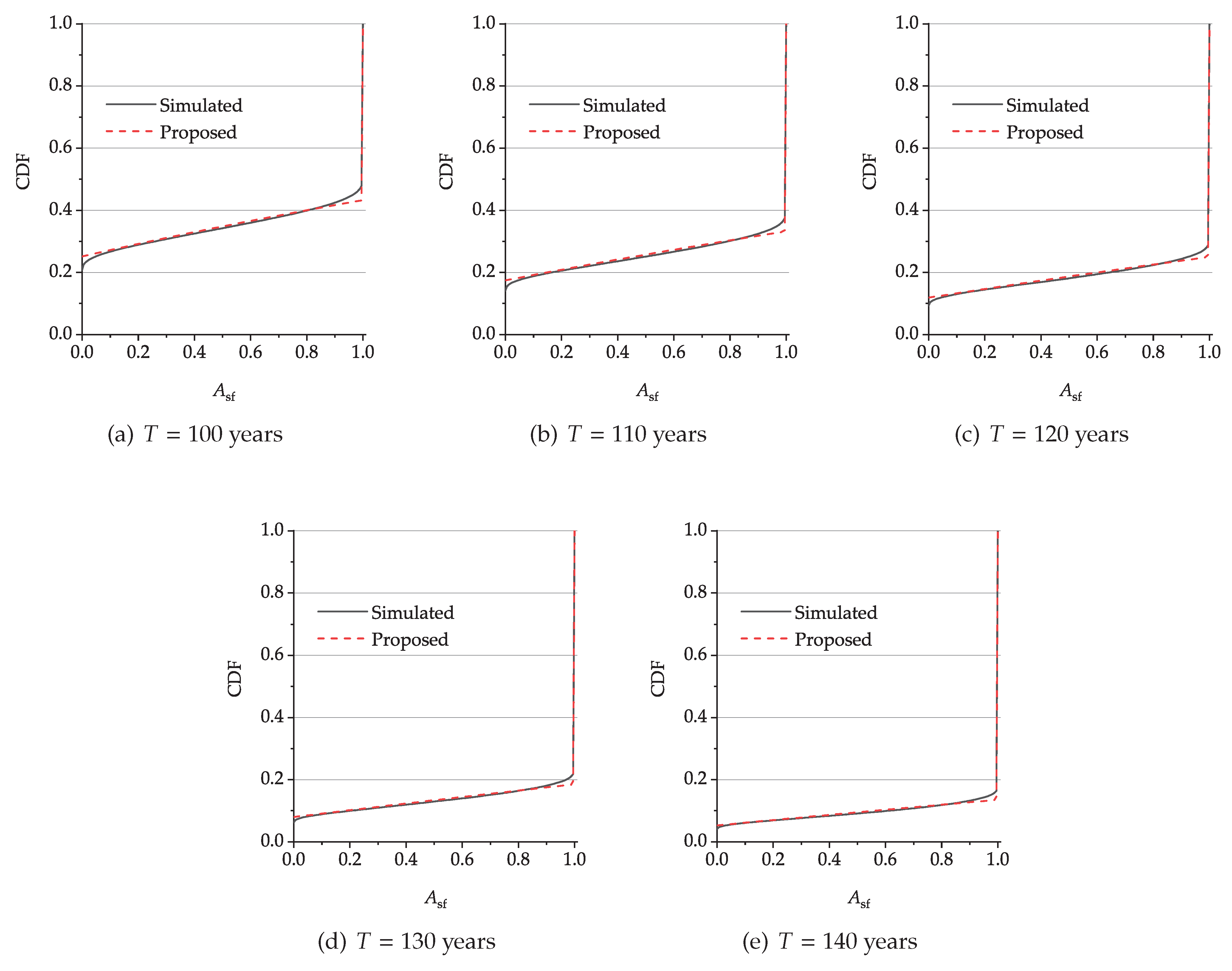
The justification for this model is two-fold. First, it aligns well with the overall behavior of
and provides an easy-to-handle approach to describe
. Second, only two parameters need to be calibrated in this model, which can be done uniquely once the mean value and variance of
are determined. Noting that the exact solution to the distribution of
could be very challenging (and may take a complicated form), the proposed model can be used to achieve a tradeoff between the accuracy and efficiency in modeling
. It is shown through a numerical example, in the next section, that the model in
Table 1 is reasonably consistent with the realistic distribution of
.
Next, the mean value and variance of
are discussed. According to Equation (
15), for a homogeneous case where the statistics of
are location-independent, it follows that:
In terms of the variance of
, by definition, one has:
Thus, the variance can be easily obtained once
is known. Based on Equation (
15),
Due to the difficulty of computing Equation (
22) directly (as it involves the summation of
items), the aim of the following derivation is to further simplify Equation (
22), which benefited from the method in [
42]. Note that the
’s associated with the
jth and
kth cells, denoted by
and
, are mutually correlated. We converted
into two standard normal variables,
and
, according to:
Let
be the correlation coefficient between
and
. We introduced a normal variable
, which is independent of
, so that:
The basis for Equation (
24) is that, the sum of two normal variables is also normally distributed. Furthermore, based on Equation (
24), the mean value and standard deviation of
are zero and
, respectively. Based on Equations (
11) and (
24), it follows that:
Using the law of total probability,
in which
is the PDF of a standard normal distribution. Substituting Equation (
26) into Equation (
22) yields,
Note that
is a function of the distance between the cells
j and
k, denoted by
ℓ. Thus,
is rewritten as
. As invoked in [
42], one can interpret Equation (
27) as the mean value of:
as
, in which
L (a random variable) is the distance between any two points within the rectangular shape
. The PDF of
L is [
43],
where:
As a result, Equation (
22) is estimated by:
Since the mean value and variance of
were readily obtained, one can further compute the two parameters involved in the probability model of
,
p and
, according to Equations (
18) and (
19). Subsequently, the reliability (or failure probability) of the surface can be calculated using Equation (
17).
The durability assessment method in Equation (
17) can also be used to guide the reliability-based inspection and repair strategies for RC structures exposed to chloride ingress, in an attempt to optimize the life-cycle costs associated with the maintenance measures for the structures. In this regard, the dynamic Bayesian network framework can be used to compute the surface reliability provided the inspection results [
11,
44,
45], where the uncertainties associated with the deterioration parameters are reduced and the surface reliability is updated dynamically.


