Buckling Instability of Monopiles in Liquefied Soil via Structural Reliability Assessment Framework

Abstract

During devastating earthquakes, soil liquefaction has disastrous outcomes on bridge foundations, as mentioned in books and published research. To avoid foundation failure when the surrounding soil is fully liquefied, a bridge’s pile foundation design could be such that the bridge pier is directly resting on the top of a large-diameter monopile instead of the traditional multiple small-diameter piles. This paper discusses the gap of insufficient studies on large-diameter monopiles to support railway bridges subjected to buckling instability and the lack of simplified tools to quickly assess structural reliability. A framework could quickly assess the structural reliability by formulating a simplified reliability analysis. This study focused on pure buckling with shear deformation and reliability assessment to calculate a monopile’s failure probability in fully liquefied soils. In reliability assessment, with the critical pile length (L_crit) and the unsupported pile length (L_uns), the limit state function g(x) = [L_crit − L_uns] thus forms the basis for assessing the safety and reliability of a structure, indicating the state of success or failure. The L_crit formulation is accomplished with a differential equation. Here, L_uns assumes various depths of liquefied soil. The reliability index’s (β) formulation is achieved through the Hasofer–Lind concept and then double-checked through a normal or Gaussian distribution. A case study was conducted using a high-speed railway bridge model from a published research to demonstrate the application of the proposed methodology. To validate the minimum pile diameter for buckling instability when a fully liquefied soil’s thickness reaches the condition that L_crit = L_uns, this study applies the published research of Bhattacharya and Tokimatsu. The validation results show good agreement for 0.85–0.90 m monopile diameters. With a monopile diameter smaller than 0.85 m, the L_crit = L_uns limit was at lesser depths, while with a monopile diameter larger than 0.90 m, the L_crit = L_uns limit was at deeper depths. A load increase notably affected the large-diameter monopiles because the L_crit movement required a longer range. In fully liquefied soil, buckling will likely happen in piles with a diameter between 0.50 m and 1.60 m because the calculated probability of failure (Pf) value is nearly one. Conversely, buckling instability will likely not happen in monopiles with a diameter of 1.80–2.20 m because the Pf value is zero. Hence, the outcome of this case study suggests that the reliable monopile minimum diameter is 1.80 m for supporting a high-speed railway bridge. Lastly, this paper analyzed the shear deformation effect on large-diameter monopiles, the result of which was 0.30% of L_crit. Shear deformation makes minimal contributions to large-diameter monopile buckling.

1. Introduction

1.1. Overview

During a highly destructive earthquake, a complex phenomenon which occurs is lateral spreading, where soil liquefaction takes place such that the soil loses its strength and appears to flow into a fluid-like material. This causes the settling, tilting, overturning, and sliding of structures on piles, such as long bridges [1] and tall buildings [2]. The damage outcomes of earthquakes have been studied for centuries, and they are mentioned in books and published research. Lateral spreading poses a significant risk to pile foundations when liquefaction affects the soil. Liquefied soil can no longer support the loads placed upon it, causing it to flow laterally. In sloping ground, this lateral movement can exert considerable force on pile foundations, potentially causing them to tilt, shift, or even fail.

Table 1. Significant historical liquefaction [3,4,5,6,7,8,9].

Date	Location	Magnitude	Comments
1925	California	6.3	The liquefaction during the Santa Barbara earthquake caused damage to the Sheffield Dam.
1964	Alaska	9.2	The effect of liquefaction during the Good Friday earthquake resulted in landslides and severe damage.
1964	Japan	7.5	Due to liquefaction, extensive damage to bridges, buildings, and port facilities in Niigata occurred.
1971	California	6.6	During the San Fernando earthquake, tremendous damage to the highway and buildings occurred.
1989	California	7.1	In San Francisco Bay, the Loma Prieta earthquake generated substantial ground amplification and damages due to liquefaction.
1994	California	6.8	The Northridge earthquake produced extreme shaking at various sites.
1995	Japan	6.9	The Hyogo-Ken Nanbu earthquake produced massive damage to Kobe.
1999	Turkey	7.4	The Kocaeli earthquake resulted in thousands of fatalities.
2008	China	7.9	A liquefaction event occurred in a densely populated area during the Wenchuan earthquake.
2010	New Zealand	7.1	Liquefaction happened during the Darfield earthquake, causing damage to a city.
2011	New Zealand	6.2	The Christchurch earthquake also caused damage to cities due to liquefaction.
2023	Turkey and Syria	7.7	On 6 February 2023, a strong earthquake doublet of Mw 7.7 and Mw 7.6 occurred in Turkey and Syria, respectively. The earthquake caused liquefaction and lateral spreading, resulting in a death toll of over 52,000 and making it the fifth-deadliest earthquake of the 21st century.

summarizes the historical events of soil liquefaction due to devastating earthquakes.

1.2. The Aftermath Impact of Earthquakes on a Transport Network

An earthquake also has a disastrous aftermath impact on transport networks, causing bridges to not be accessible for rescue operations or relief goods delivery to the affected areas. As such, a bridge’s structure must be structurally efficient [10]. However, in areas prone to soil liquefaction, the increase in pore pressure will decrease the strength of soil and its stiffness, which seriously affects the pile foundation’s response to ground shaking [11], resulting in significant bending moments and buckling (see Figure 1b) which threaten the pile’s structural stability [12]. Instead of several piles of a small diameter, as shown in Figure 1a, the bridge’s pile foundation design could be such that the bridge pier is directly resting on the top of a large-diameter monopile, as illustrated in Figure 1c. However, this type of foundation might experience pure buckling instability with a shear deformation effect. Some bridge projects applied monopile foundations because of restricted spaces and congested locations [13]. Also, this could minimize existing utility conflicts [14] and avoid the risk of pile cap splitting due to an active fault line [15].

2. Literature Review

During seismic liquefaction, the various feasible pile failure mechanisms are shear, bending, buckling, and cyclical loading [16]. However, this literature review focused on pure buckling instability with the shear deformation effect.

Pile bending or flexural mechanism is a well-established theory based on the assumption that piles act as laterally and axially loaded “beams” during liquefaction [17,18,19]. On the contrary, a theory on buckling instability assumes that piles behave as axially loaded “columns” in liquefied soil, and some researchers verified this hypothesis through experimentation [20,21,22].

Designing piles to resist bending as a beam and buckling as a cantilevered column requires different approaches; the former relies on the pile’s strength [23], and the latter relies on its stiffness [24]. Increasing the pile’s yield strength is advisable to steer clear of bending failure. However, this may not be sufficient to prevent the piles from buckling [25]. A pile may bend due to lateral loading. However, some researchers considered this scenario to be secondary to the necessity that piles in liquefiable soils must be examined for Euler’s buckling load because soil loses its strength when liquefied. The lateral load is minimal compared with the axial load [26]. In analyzing pile bending and buckling in liquefied soil, the commonly used mathematical approach is the Euler–Bernoulli theory [27]. However, other researchers found out that the Euler–Bernoulli theory does not provide realistic analysis for large-diameter monopiles because the effect of shear deformation is not considered [28].

Various studies revealed the outcomes of considering the effect of shear deformation in pile analysis. For example, Han and Frost [29] compared a pile’s lateral deformation due to combined axial and lateral load using the subgrade reaction approach, in which they noticed more significant pile deflections when employing Timoshenko’s theory. Gupta and Basu [30] used the Euler-Bernoulli, Timoshenko, and rigid beam theories in analyzing laterally loaded piles. They observed in some cases that the Euler–Bernoulli theory underestimated the deformation of the pile head. Furthermore, Bechtel et al. [31] studied a polymer pile’s lateral response using the finite element method, in which they concluded that the shear deformation effect is relevant and suggested adding it to the analysis of pile design. However, most of these works used complex mathematical approaches and did not consider the probabilistic measure of structural safety through the structural reliability of the pile foundation.

On the other hand, a structural reliability assessment is essential to know the probability of failure, owing to the buckling instability of piles in liquefied soils, including the shear deformation effect. The structure’s ability to comply with given requirements under specific conditions [32] is one of the definitions of structural reliability. Theoretically, structural failures may happen once the structure’s capacity minus demand exceeds the limit state. A structure’s acceptable behavior is when the limit state function g(x) has a resulting value less than zero, thus indicating a safe domain [33].

Research progress in reliability analysis concerning buckling instability, especially in structural engineering contexts, has evolved significantly in recent years. There has been a shift toward probabilistic modeling [34] to account for uncertainties in material properties, geometric imperfections, loading conditions, and environmental factors. Advanced techniques such as Monte Carlo simulation [35] and response surface methodology [36] are employed to assess the reliability of structures under buckling conditions. Also, some design codes are evolving to include reliability-based approaches for assessing buckling instability [37]. These codes provide guidelines for probabilistic structural performance assessment under different loading scenarios, ensuring safety margins are appropriately defined. However, most of these studies are for buildings and not large-diameter monopiles supporting railway bridges.

The gap in the knowledge that exists in the current literature consists of (1) insufficient studies on large-diameter monopiles supporting railway bridges subjected to buckling instability during seismic liquefaction and (2) a lack of simplified tools to quickly assess the structural reliability of large-diameter monopile foundations for railway bridges. This study aims to tackle this gap by formulating a simplified framework which considers the critical pile length for the capacity of the pile foundation, with the unsupported pile length as the demand. This simplified framework can quickly assess the structural reliability of large-diameter monopiles in fully liquefied soil which causes buckling instability failure.

Text Structure

The outline of this review is as follows.

Section 1 introduces the study’s overview in a broader context by presenting damaging outcomes of earthquakes resulting in soil liquefaction. This section highlights the possibilities of a bridge pier directly resting on top of a large-diameter monopile instead of several smaller-diameter piles.

Section 2 discusses the literature review. However, it focuses on pure buckling instability with the shear deformation effect. The gap in the knowledge that exists in the current literature consists of (1) insufficient studies on large-diameter monopiles supporting railway bridges subjected to buckling instability during seismic liquefaction and (2) a lack of simplified tools to quickly assess the structural reliability of large-diameter monopile foundations for railway bridges.

Section 3 illustrates the mathematical formulation framework of the current study.

Section 4 shows a case study of a high-speed railway bridge model to demonstrate the application of the proposed methodology illustrated in Section 3.

Section 5 shows the results and discussions. This section presents the validation of the current study using the information from published research, namely the current study pile length comparison, probability of failure analysis, and the effect of shear deformation.

Section 6 presents the concluding statements. There is a need for further research to fill the gaps in the study of monopiles during the transient stage, a short period from a phase with no soil liquefaction to a fully liquefied soil phase. Also, this section mentions the limitations of the current study.

3. Methodology

3.1. Mathematical Formulation Framework

The methodology adopted in this research is based on the first-order reliability method, also known as the Hasofer-Lind Reliability Index [38]. It is a semi-probabilistic way of evaluating structural reliability for a linear state function. This method is advantageous because it avoids the ambiguities associated with contrasting formulations of the limit state function [39]. The framework is composed of two independent streamlines, as illustrated in Figure 2. Streamline 1 at the left-hand side of the illustration aims to formulate the capacity by considering the critical pile length, depending on the intensity of the dynamic load at the top of the monopile in a surrounding liquefied soil. Streamline 2 on the right-hand side aims to determine the demand by considering the unsupported pile length, which equals the liquefied soil depth. Then, the calculated critical pile length and unsupported pile length are the input data for evaluating the probability of failure of a monopile in fully liquefied soil conditions. On the other hand, a reliability index is an essential parameter for measuring structural reliability instead of the probability of failure. Appendix A summarizes the notation used in the current study.

3.2. Critical Pile Length Formulation

The static axial load (P_stat) is the load of the structure which is safely resting above the pile foundation. However, when an earthquake strikes, the structure’s inertial action obtrudes a dynamic axial load (P_dyn) which is often much greater than the structure’s static equivalent [25], which may cause the pile foundation to buckle. To estimate the maximum axial load on top of a pile, refer to Equation (1):

$$P_{dyn}=P_{stat}+{\alpha P}_{stat}=(1+\alpha )P_{stat}$$

(1)

Here, the Greek letter $\alpha$ is the dynamic amplification factor, which is a function of the structure’s type, the center of its mass, and earthquake excitation responses.

The possible effect of an earthquake on pile foundations is that the pile becomes laterally unsupported in the layer of liquefiable soil because it loses its lateral restraint from the surrounding ground [16,25]. Thus, the pile is vulnerable to buckling failure once its axial load increases from P_stat to P_dyn. Hence, there shall be three scenarios for the critical pile length (L_crit) and unsupported pile length (L_uns) hypothesis, as illustrated in Figure 3. Here, L_crit is the length of a pile at which buckling instability occurs under a specific load, such as P_dyn. Beyond this L_crit value, the pile becomes susceptible to buckling failure. The L_uns value is the soil’s weak region which may fully liquefy during an earthquake. Also, this portion of the pile at L_uns loses its lateral support and is susceptible to buckling. The pile fixity depth (D_fix) is the pile’s embedded length in the hard strata. Soil_liquid represents the liquefied soil profile, Soil_hard is the non-liquefied hard strata, and d is the minimum pile diameter to support the P_dyn against buckling instability.

In Figure 3a, Case 1 represents a condition where L_crit extends farther down than L_uns. In this case, the pile has a higher chance of withstanding the effect of P_dyn in the surrounding Soil_liquid during an earthquake. However, D_fix could be greater than required and, therefore, overdesigned. In Figure 3b, Case 2 shows when L_crit has the same depth as L_uns, in which the pile is at its minimum requirement to sustain P_dyn in the surrounding Soil_liquid [40]. In Figure 3c, Case 3 shows an unsafe condition for the pile, where L_uns extends farther down than L_crit, which may result in buckling instability failure.

The structural analysis of a pile in liquefied soil as a column element carrying an axial load is often more realistic than treating it as a beam element carrying the same load, especially in certain geotechnical conditions [20,21,22]. The technical reason for this is that the pile’s behavior in liquefied soil is significantly influenced by the surrounding soil’s response to liquefaction. Analyzing it as a column element carrying an axial load might be more appropriate in this context because this focuses on the vertical load-carrying capacity of the pile. A minimum pile diameter, represented by the letter d, should correspond with the depth of the liquefied soil to prevent the pile from undergoing column buckling failure. When comparing the critical pile length with the unsupported pile length, the potential pile failure due to buckling instability shall be when L_crit < L_uns, as depicted in Case 3 of Figure 3c.

On the other hand, the monopile’s ability to comply with structural reliability under certain geotechnical conditions, such as the probability of failure due to the monopile’s buckling instability in liquefied soils, may happen once the monopile’s capacity minus demand exceeds the limit state. Accordingly, the structure’s acceptable behavior is when the limit state function g(x) has a resulting value less than zero. Thus, this indicates that it is in a safe domain [33]. Here, g(x) is a fundamental structural engineering and reliability analysis concept. It is a key component in the design and analysis of structures to ensure that they can safely withstand anticipated loads and environmental conditions. For the structural reliability assessment of a monopile, refer to Equation (2), where L_crit is the capacity term while L_uns is the demand:

$$g\left(x\right)=[L_{crit}-L_{uns}]$$

(2)

The monopile is safe when the limit state function (g(x)) equals a positive value. Otherwise, the monopile is unsafe when g(x) results in a negative value.

The critical axial load for a monopile foundation is found by considering a hypothetical column performance, assumed at first to be ideally straight and compressed by an axial load. From the elementary beam theory point of view, the stresses and deflections are directly proportional to the applied load. The expression of the curvature of the axis of a vertical beam element delineated in Figure 3c shall be as shown in Equation (3):

$$EI{\displaystyle \frac{d^{2}x}{d{y}^2}}=-M$$

(3)

Here, the representation of E is the elastic modulus, I is the moment of inertia, and M is the bending moment. On the other hand, when the coordinate axes are taken as indicated in Figure 3c, and the pile is assumed to be a column element with a slightly deflected position, the bending moment at any cross-section a-b becomes as shown in Equation (4):

$$P(\delta -x)=-M$$

(4)

To calculate the critical axial load which a column element can carry, the axial force (P) multiplied by the displacement $(\delta -x)$ at any cross-section shall equal the bending moment. When combining Equation (3) with Equation (4), the resulting equation is Equation (5):

$${\displaystyle \frac{d^{2}x}{d{y}^2}}={\displaystyle \frac{P(\delta -x)}{EI}}$$

(5)

However, the value of P should be the minimum axial force or the critical load when a column starts buckling.

In 1744, Leonhard Euler introduced a theory regarding the critical axial load (P_cr) or Euler’s critical load [41] (refer to Equation (6)). This is the minimum compressive axial load which causes a column to buckle. The assumptions for Euler’s theory are as follows: (1) the column is ideally straight; (2) the cross-section is uniform; (3) the material is homogeneous and elastic; and (4) the compressive force acts on the centroid of the section:

$$P_{cr}={\displaystyle \frac{{\pi }^{2}EI}{{\left(KL\right)}^2}}$$

(6)

where L is the unsupported column length and K represents the column’s effective length factor. Considering that the axial load P in Equation (5) equals P_cr in Equation (6), when combining these equations, the result is Equation (7):

$${\displaystyle \frac{\raisebox{1ex}{$d^{2}x$}\!\left/ \!\raisebox{-1ex}{${dy}^2$}\right.}{(\delta -x)}}={\displaystyle \frac{{\pi }^2}{{\left(KL\right)}^2}}$$

(7)

However, the mathematical expressions introduced in Equations (3)–(7) neglect the effect of a shearing force in deriving the deflection curve using a differential equation. Based on a book by Timoshenko and Gere [42], shearing forces act on the column’s cross-section when buckling happens, as illustrated in Figure 4.

The shearing force $\left(Q\right)$ presented in Figure 4b, which is normal to the column’s axis, conforms to the element of the length dy between two cross-sections a and b. The corresponding equation of a shearing force is shown in Equation (8):

$$Q=P{\displaystyle \frac{dx}{dy}}$$

(8)

By applying the differential equation, this becomes Equation (9):

$${\displaystyle \frac{dQ}{dy}}=P{\displaystyle \frac{d^{2}x}{d{y}^2}}$$

(9)

Merging the change in the deflection curve’s slope due to the shearing force of $nQ/AG$ thus creates the equation for the shear deformation through multiplying the left-hand side of Equation (9) by a numerical factor (n) and dividing this by the cross-sectional area (A) with a shear modulus (G), which will form Equation (10):

$$n\left({\displaystyle \frac{dQ}{dy}}\right)/AG$$

(10)

For a circular cross-section, Timoshenko and Gere [42] considered a value of n equal to 1.11. By substituting the value of dQ/dy in Equations (9) and (10), the curvature created by the shearing force is as expressed in Equation (11):

$$n\left(P{\displaystyle \frac{d^{2}x}{d{y}^2}}\right)/AG$$

(11)

Hence, obtaining the total curvature of the deflection curve (d²x/dy²) is achieved by incorporating the curvature produced by the shearing force into the curvature created by the bending moment. For the column shown in Figure 4, the differential equation of the deflection curve shall be the combination of Equations (5) and (11), which generates Equation (12a) and then creates Equation (12b):

$${\displaystyle \frac{d^{2}x}{d{y}^2}}=P{\displaystyle \frac{(\delta -x)}{EI}}+n\left(P{\displaystyle \frac{d^{2}x}{d{y}^2}}\right)/AG$$

(12a)

$${\displaystyle \frac{\raisebox{1ex}{$d^{2}x$}\!\left/ \!\raisebox{-1ex}{$d{y}^2$}\right.}{(\delta -x)}}={\displaystyle \frac{P}{EI\left(1-\frac{nP}{AG}\right)}}$$

(12b)

Combining Equations (7) and (12b) will generate Equation (13). On the left-hand side of this equation, it is noticeable that it is equivalent to Euler’s critical load, shown in Equation (6). We rename P_cr to Pe to represent the critical load or Euler’s buckling formula without shear deformation. Furthermore, we rename P to P_cr+s, representing the critical axial load with the effect of shear deformation (refer to Equation (14)):

$${\displaystyle \frac{{\pi }^{2}EI}{{\left(KL\right)}^2}}={\displaystyle \frac{P}{\left(1-\frac{nP}{AG}\right)}}$$

(13)

$$P_{cr+s}={\displaystyle \frac{Pe}{1+\left(\frac{n}{AG}\right)Pe}}$$

(14)

In the critical pile length and unsupported pile length hypothesis illustrated in Figure 3, the maximum P_dyn which causes the pile to buckle—that is, the load at which the pile may fail (P_fail)—should not be equal to P_cr+s because there are uncertainties and imperfections to be considered in the analysis. Hence, P_fail shall be less than P_cr+s (refer to Equation (15)):

$$P_{fail}<P_{cr+s}$$

(15)

The value of P_fail can be determined by multiplying P_cr+s by a reduction factor ($\varnothing$) to obtain more conservative assumptions in the analysis (refer to Equation (16)):

$$P_{fail}=\varnothing P_{cr+s}$$

(16)

Multiplying the calculated P_cr+s by $\varnothing$ ensures good safety in P_fail’s determination. The reduction factor shall be less than one ($\varnothing$ < 1) to adjust a certain risk’s estimated impact or reduce the likelihood of failure.

In the condition of a monopile failure’s limit state, the load P_dyn due to earthquake shaking shall equal P_fail or the axial load which may cause the monopile to buckle, as illustrated in Figure 3c. Putting Equations (14) and (16) together will generate Equation (17):

$$P_{dyn}=\varnothing \left[{\displaystyle \frac{Pe}{1+\left(\frac{n}{AG}\right)Pe}}\right]$$

(17)

The magnitude of P_dyn equals (1 + $\alpha$) P_stat, as defined in Equation (1), while Pe equals Euler’s critical load, as presented in Equation (6). By, letting L equal L_crit, the generated equation is Equation (18):

$${\left(1+\alpha \right)P}_{stat}=\varnothing \left[{\displaystyle \frac{\frac{{\pi }^{2}EI}{K^2{L_{crit}}^2}}{1+\left(\frac{n}{AG}\right)\left(\frac{{\pi }^{2}EI}{K^2{L_{crit}}^2}\right)}}\right]$$

(18)

Extracting the mathematical expression of L_crit from Equation (18) shall lead to formulating Equation (19) in determining the critical pile length, considering buckling instability due to an actual failure axial load with the shear deformation effect:

$$L_{crit}=\sqrt{{\displaystyle \frac{{\pi }^{2}EI\left[\varnothing -\left(\left(\left(1+\alpha \right)P_{stat}\right)\left(\frac{n}{AG}\right)\right)\right]}{K^2\left[\left(1+\alpha \right)P_{stat}\right]}}}$$

(19)

Also, this research intends to investigate the difference in the mathematical expression of L_crit without shear deformation effects. The value of P_fail shall be less than the force Pe (refer to Equation (20)), corresponding to the magnitude of P_dyn, which is equivalent to the reduced Pe (refer to Equation (21)):

$$P_{fail}<Pe$$

(20)

$$P_{dyn}=\varnothing Pe$$

(21)

To generate Equation (22) from Equation (21), let P_dyn equal (1 + α)P_stat on the left-hand side, and then substitute Pe with Equation (6), which is equivalent to P_cr on the right-hand side. Then, let L equal L_crit:

$${\left(1+\alpha \right)P}_{stat}=\varnothing \left[{\displaystyle \frac{{\pi }^{2}EI}{K^2{L_{crit}}^2}}\right]$$

(22)

In Equation (22), the L_crit formulation is represented by Equation (23):

$$L_{crit}=\sqrt{{\displaystyle \frac{{\pi }^{2}EI\left[\varnothing \right]}{K^2\left[\left(1+\alpha \right)P_{stat}\right]}}}$$

(23)

The dissimilarities between Equations (19) and (23) are noticeable. In Equation (19), the term [$\varnothing$ − (((1 + α)P_stat) (n/AG))] indicates that a shearing force deducts the reduction factor, but in Equation (23), the term [$\varnothing$] is not deducted. These formulation dissimilarities specify that adding the effect of shear deformation will significantly increase the safety factor because the value of the reduction factor shall be decreased. Moreover, the estimated value of the critical pile length, including the shear deformation, is lower than the critical pile length when not considering shear deformation. Accordingly, L_crit depends on the intensity of P_dyn at the top of the monopile in liquefied soil.

The essential parameters needed in Equations (19) and (23) are $\varnothing$, K, n, and α. Some studies considered the pile’s buckling instability with a $\varnothing$ value of 0.35 [25]. It is necessary to evaluate a pile regarding its boundary condition, such as fixed, pinned, or free end, in which the value of K for the column with a fixed end at the base and a free end at its top is 1.00 [12]. Drilled monopiles are practically circular cross-sections. The assumed value of n for a circular section is 1.11 [42]. At the top of the pile, the acceleration amplification factor stabilizes at 1.32 [43]. However, conducting a sensitivity analysis of ∅, K, n, and α using books, conference papers, articles, and published research is advisable.

3.3. Unsupported Pile Length Formulation

The assumptions in determining the unsupported pile length (L_uns) equal the liquefied soil depth. Liquefaction determination has two methods: magnitude plots versus the epicentral distance [44] and the simplified procedure [45]. However, the first method uses approximation, which is suitable as a screening guide, while the other is a detailed method. Furthermore, these two methods are not akin.

Liquefaction can occur down to a 20 m depth. However, the chances of this are not the same in different soil layers. This phenomenon is potentially high on the surface and linearly decreases to a depth of 20 m [6]. The liquefaction potential index (LPI) formulation provided by Iwasaki et al. [46] is shown in Equation (24):

$$LPI={\int }_0^{20}F\left(z\right)w\left(z\right)dz$$

(24)

where F(z) represents the severity function, which equals the function of the factor of safety (FS) in anticipation of liquefaction, and w(z) is a weighting factor. The value of w(z) (refer to Equation (25)) is 10 for the surface level or at natural ground level and 0 beyond a 20 m depth, as liquefaction will likely not happen after 20 m deep in soil. Z represents the soil depth in meters and should not exceed 20 m:

$$w\left(z\right)=10-0.5\left(Z\right)$$

(25)

Galupino and Dungca [47] presented an estimate of the function of FS against liquefaction or the so-called probability of liquefaction (PL), which is shown in Equation (26):

$$PL={\displaystyle \frac{1}{1+{\left(\frac{FS}{0.96}\right)}^{4.5}}}$$

(26)

The computations for the FS in different layers of soil shall be in terms of the cyclic shear stress ratio, cyclic resistance ratio and magnitude scaling factor. However, there are many arguments in the literature that soil shall liquefy until FS = 1.20 [6], while other studies adopted 1 < FS < 1.2 [48]. When merging Equation (25) with Equation (24) and letting PL = F(z), the resulting generated equation is Equation (27):

$$LPI={\int }_0^{20}PL[10-0.5\left(Z\right)]dz$$

(27)

Then, the probability of ground failure (P_G) [49] using a quantitative assessment [50] shall become Equation (28):

$$P_G={\displaystyle \frac{1}{1+e^{4.71-0.71\left(LPI\right)}}}$$

(28)

3.4. Limit State Function Formulation Using the Hasofer–Lind Reliability Index

The term L_crit is the capacity, while L_uns is the demand. Then, the failure criterion is g(x) = [L_crit − L_uns], which is the limit state function, as explained in Equation (2). Structural reliability assessment aims to evaluate the probability of failure (P_f) of a monopile in liquefied soil conditions. On the contrary, a reliability index (β) is an essential parameter for measuring structural reliability, unlike P_f.

In 1974, Hasofer and Lind [38] developed the Hasofer-Lind Reliability Index, also recognized as the first-order reliability method (FORM). It is a semi-probabilistic way of evaluating structural reliability, described as the closest distance from the intersection of the Y₁ and Y₂ axes to the failure surface. This method is advantageous because it avoids the ambiguity of using the first-order second method (FOSM) associated with contrasting formulations of the limit state function [39].

In determining the value of β using the Hasofer–Lind Reliability Index, we convert the random variables X = {X₁, X₂, …, X_n} into Y = {Y₁, Y₂, …, Y_n} as shown in Equation (29). The variables comprising Y are the standard normal variables with a mean equal to zero and a unit standard deviation. The conversion is easy if X is an independent random variable, which resolves the lack of invariance problem:

$${\mathrm{Y}}_i={\displaystyle \frac{{\mathrm{X}}_i-{\mu }_{{\mathrm{X}}_i}}{{\sigma }_{{\mathrm{X}}_i}}}$$

(29)

The original coordinate system X is equal in function to the converted or transformed coordinate system Y. Then, the limit state function changes from the original g(x) to a transformed g(y). Figure 5 presents the Hasofer–Lind transformation of the original coordinate system X to a converted coordinate system Y.

As shown in Figure 5b, the closest point with the shortest line to the limit state surface Y* is the checking or design point, in which this line represents the values of the reduced random variable. Figure 5a shows that the borderline between failure and safe spaces is g(x) = 0. The random variables X₁ and X₂ represents L_crit and L_uns respectively. By utilizing Equation (29) these variables shall be converted into reduced random variables Y₁ and Y₂, resulting to Equations (30) and (31):

$${\mathrm{X}}_1={\mu }_{{\mathrm{X}}_1}+{\sigma }_{{\mathrm{X}}_1}{\mathrm{Y}}_1$$

(30)

$${\mathrm{X}}_2={\mu }_{{\mathrm{X}}_2}+{\sigma }_{{\mathrm{X}}_2}{\mathrm{Y}}_2$$

(31)

The formulation of the transformed limit state function (g(y)) is the merging of Equations (30) and (31) into Equation (2), as illustrated in Figure 4a, which is borderline in the middle of the failure and safe spaces. This concept generates Equation (32a,b):

$$g\left(x\right)={\mathrm{X}}_1-{\mathrm{X}}_2=0$$

(32a)

$$g\left(y\right)={\mu }_{{\mathrm{X}}_1}+{\sigma }_{{\mathrm{X}}_1}{\mathrm{Y}}_1-{\mu }_{{\mathrm{X}}_2}-{\sigma }_{{\mathrm{X}}_2}{\mathrm{Y}}_2=0$$

(32b)

The line g(y) = Y₁ − Y₂ = 0 in Figure 4b represents the limit state surface, which is the borderline in the middle of the failure and safe spaces. If the location of the line g(y) is nearer to the origin of the converted or transformed coordinate system, then the failure space is more extensive and contrariwise. Accordingly, the closest distance β directly linked to P_f characterizes the location of the line g(y) in the transformed coordinate system regarding the system’s origin. The coordinates of the line g(y) which intercept with the transformed coordinate axes Y₁ and Y₂ are the points for obtaining the formula for β using a simple geometry considering an isosceles triangle with two sides of equal length, in which the mathematical form to determine β for the Hasofer–Lind Reliability Index shall be as expressed in Equation (33):

$$\beta ={\displaystyle \frac{{\mu }_{{\mathrm{X}}_1}-{\mu }_{{\mathrm{X}}_2}}{\sqrt{{\sigma }_{{{\mathrm{X}}_1}^2}+{\sigma }_{{{\mathrm{X}}_2}^2}}}}$$

(33)

Furthermore, this research explores the reliability index derived using the normal or Gaussian distribution. One of the exceptional cases is when the P_f analysis is not complicated, in which X₁ and X₂ are considered independent normal random variables. Equation (32a) is equivalent to a normal random variable with its means and variances. The resulting equation for the means is Equation (34), while that for the variance is Equation (35a), which is equivalent to Equation (35b):

$${\mu }_{g\left(x\right)}={\mu }_{{\mathrm{X}}_1}-{\mu }_{{\mathrm{X}}_2}$$

(34)

$${{\sigma }_{g\left(x\right)}}^2={{\sigma }_{{\mathrm{X}}_1}}^2+{{\sigma }_{{\mathrm{X}}_2}}^2$$

(35a)

$${\sigma }_{g\left(x\right)}=\sqrt{{{\sigma }_{{\mathrm{X}}_1}}^2+{{\sigma }_{{\mathrm{X}}_2}}^2}$$

(35b)

Here, μ_X1 and μ_X2 represent the means while σ_X1 and σ_X2 are the standard deviations of X₁ and X₂, respectively. The simplest case of modeling X₁ and X₂ as two random variables is using the probability distributions f_X1(X₁) and f_X2(X₂), respectively, in which P_f shall be as expressed in Equation (36a,b):

$$P_f=P\left(g\right(x)\le 0)$$

(36a)

$$P_f=P({\mathrm{X}}_1-{\mathrm{X}}_2\le 0)$$

(36b)

The probability distribution function (PDF) utilizing the concept of the normal distribution is Equation (37):

$$f_x\left(\mathrm{X}\right)={\displaystyle \frac{1}{\sqrt{2\pi \sigma }}}{e}^{\left(-{\displaystyle \frac{1}{2}}{\left({\displaystyle \frac{\mathrm{X}-\mu }{\sigma }}\right)}^2\right)}$$

(37)

where μ represents the mean while σ is the standard deviation of the variable X. Here, ${\displaystyle \frac{1}{\sqrt{2\pi }}}$ ensures that the area under the PDF equals one. The rationale of the random variable X is in the gamut of infinities (−∞, ∞). We replace the random variable X with a comparable normalized expression (U) (refer to Equation (38)) to derive the standard form of this distribution:

$$U={\displaystyle \frac{\mathrm{X}-\mu }{\sigma }}$$

(38)

When merging the standard form presented in Equation (38) with Equation (37), the generated PDF shall be as expressed in Equation (39):

$$f_u\left(U\right)={\displaystyle \frac{1}{\sqrt{2\pi }}}{e}^{\left(-{\displaystyle \frac{U^2}{2}}\right)}$$

(39)

The mathematical forms of the cumulative distribution function (CDF) are as shown in Equation (40a–c):

$$F_x\left(\mathrm{X}\right)=P(\mathrm{X}\le x)$$

(40a)

$$F_x\left(\mathrm{X}\right)=\Phi \left({\displaystyle \frac{\mathrm{X}-\mu }{\sigma }}\right)$$

(40b)

$$F_x\left(\mathrm{X}\right)=\Phi \left(U\right)$$

(40c)

By letting Equation (36a) equal Equation (40b) and considering the values of X = 0, μ = μ_g(x), and σ = σ_g(x), the generated equation shall be as shown in Equation (41):

$$P_f=\Phi \left(-{\displaystyle \frac{{\mu }_{g\left(x\right)}}{{\sigma }_{g\left(x\right)}}}\right)=\Phi \left(-\beta \right)$$

(41)

In Equation (41), the equivalent mathematical expression for the structural reliability index is as shown in Equation (42):

$$\beta ={\displaystyle \frac{{\mu }_{g\left(x\right)}}{{\sigma }_{g\left(x\right)}}}$$

(42)

When incorporating Equation (34) and Equation (35b) into Equation (42), the resulting equation is Equation (43):

$$\beta ={\displaystyle \frac{{\mu }_{{\mathrm{X}}_1}-{\mu }_{{\mathrm{X}}_2}}{\sqrt{{\sigma }_{{{\mathrm{X}}_1}^2}+{\sigma }_{{{\mathrm{X}}_2}^2}}}}$$

(43)

It is noticeable that Equation (43) and Equation (33) end with the same mathematical expressions. Gowever, the formulation of each equation uses a different approach. The former uses simple geometry, while the latter uses the properties of the independent normal random variables X₁ and X₂. When the limit state function is a linear operation of two variables X₁ and X₂ or L_crit and L_uns, both descriptions provide a similar mathematical form of reliability index.

In summary, when combining Equation (33) with Equation (41), the structural reliability which corresponds to the probability of failure for a monopile buckling in liquefied soils is as shown in Equation (44):

$$P_f=\Phi \left(-{\displaystyle \frac{{\mu }_{L_{crit}}-{\mu }_{L_{uns}}}{\sqrt{{\sigma }_{{L_{crit}}^2}+{\sigma }_{{L_{uns}}^2}}}}\right)$$

(44)

Here, Φ (.) represents the standard normal distribution CDF, for which the tabulated values are ready for use in standard textbooks or the Excel program (=NORMSDIST(.)). The term inside the CDF, (−β), is the reliability index. The transformed coordinate system, illustrated in Figure 4b by Hasofer and Lind, can be further developed to visually indicate the limit state surface because it is an isosceles triangle representation. If the perpendicular distance from the longest side of the triangle to the (0,0) origin is farther, then this might indicate a lower likelihood of failure. However, if the perpendicular distance from the longest side of the triangle to the origin is too close, then this might indicate a greater likelihood of failure, and this requires further studies.

4. Case Study

The structural reliability assessment via the probability of failure of a monopile foundation’s buckling instability in liquefied soil is like a structural system relying on a column element cantilevered from a fixed base and free at the top with axial force applied centrically.

A case study of a high-speed railway (HSR) bridge model was used to demonstrate the application of the proposed methodology illustrated in the previous section. This case study consisted of a five-span, simply supported box girder bridge. The bridge deck and pier column’s cross-sectional dimensions can be seen in the published research of Chen et al. [51]. The 32 m deck was a prestressed concrete box girder of a trapezoidal cross-section. The reinforced concrete solid pier columns were 10–20 m high, with round-end cross-sections resting on a concrete drilled pile foundation with circular sections. The HSR bridge model assumed a fully fixed rigid connection between the pier column and monopile foundation, in which the pier column remained elastic during earthquake shaking.

Table 2. Geometric parameters of the model [51].

Parameters	Value
Length of girder	32 m
Width of girder	12 m
Height of girder	3.05 m
Area of girder	8.6597 m2
Linear mass of girder	2.19 × 104 kg/m
Length of pier column in cross-section	6.20 m
Width of pier column in cross-section	2.20 m
Height of pier column nos. 1–6	10 m, 12 m, 14 m, 16 m, 18 m, and 20 m
Area of solid pier (round-shaped)	11.141 m2
Unit weight of concrete	24 kN/m3
Superimposed dead load	184 kN/m

outlines the parameters of the HSR bridge. This type of bridge represents more than 90% of China’s HSRs.

Table 3. Parameters from various research.

Parameters	Value	From the Study by
E	25,000,000 KPa	Moayedi et al. [52]
$\varnothing$	0.35	Bhattacharya [25]
n	1.11	Timoshenko and Gere [42]
α	1.32	Dong et al. [43]
ν	0.2	Pal [53]
K	1.00	Madabhushi et al. [12]
Train load	83.60 kN/m	Aziz and Ma [54]

consists of other parameters used in this study: the elastic modulus (E), reduction factor ($\varnothing$), numerical factor (n), amplification factor (α), Poisson’s ratio (ν), and column’s effective length factor (K), as well as the train load or live load from the bridge to the foundation.

This paper applied the abovementioned parameters to illustrate Equation (19) for L_crit with shear deformation and Equation (23) for L_crit without shear deformation, considering various monopile diameters of 0.50 m, 0.60 m, 0.70 m, 0.85 m, 0.90 m, 1.10 m, 1.40 m, 1.60 m, 1.80 m, 2.00 m, and 2.20 m. The selected monopile diameters were based on Bhattacharya and Tokimatsu’s published research [40]. The current study used the same sets of pile diameters for validation purposes. This case study considered a pile fixity depth (D_fix) sufficiently anchored on hard strata to secure the pile bottom, factoring in no settlement and overturning.

Table 4. Parameters for the probability of failure.

Parameters	Value
μLcrit	Based on the calculated Lcrit, which depends on various pile diameters, and Pdyn generated from Table 2.
μLuns	10.00 m
σLcrit	Based on the calculated Lcrit, which depends on various pile diameters, and Pdyn generated from Table 2.
σLuns	7.74798

presents the parameters to illustrate Equation (44) for the probability of failure of a monopile and assess its structural reliability. The value of the mean of the critical pile length (μL_crit) was calculated based on L_crit, which is dependent on the pile diameter and axial load P_dyn. L_uns was assumed to be five depths of liquefiable soil—0.25 m, 5 m, 10 m, 15 m, and 19.75 m—in which the value of the mean of unsupported pile length (μL_uns) was 10.00 m. Eventually, the standard deviations (σL_crit) and (σL_uns) would be calculated from the provided data of L_crit and L_uns, respectively. The five selected depths were based on the fact that the liquefaction phenomenon is potentially high on the surface and linearly decreases to a depth of 20 m [6]. For a preliminary liquefaction analysis, it is common to consider the upper 9 m of soil. If the liquefaction potential is a significant concern, then a more detailed analysis may need to be performed for site-specific investigations.

5. Results and Discussion

5.1. Current Study Validation

The current study conceptualized that when L_crit has the same depth as L_uns during liquefaction, as depicted in Figure 3b, the monopile is at its minimum capacity in supporting the axial load P_dyn in Soil_liquid because it is at the limits between the safe and unsafe states. Figure 6 shows the results of L_crit with the shear deformation effect using Equation (19), contingent on the pile diameter and axial load P_dyn for selected pier column heights of 10 m and 20 m. In addition, this paper applied the published research of Bhattacharya and Tokimatsu [40] to validate the minimum pile diameter for buckling instability when a fully liquefied soil’s thickness reaches the L_crit = L_uns condition.

The validation outcome indicates good agreement for monopile diameters of 0.85–0.90 m in that the estimated L_crit = L_uns condition occurred in depths 6.69–8.05 m from the natural ground level. However, with smaller monopile diameters of 0.50 m to 0.70 m, the estimated L_crit = L_uns condition was at lesser depths than those in Bhattacharya and Tokimatsu’s study. On the other hand, with larger pile diameters of 1.10 m to 2.20 m, the estimated L_crit = L_uns condition was deeper than suggested. For example, the 1.80 m monopile diameter should start to buckle at a 16 m depth [40]. However, this study estimated that the monopile started buckling when L_crit = L_uns reached 30.29 m in depth. The deepest reach of liquefaction was 20 m in depth [46], for which the suggested diameter was 2.20 m [40]. However, the current study estimated a minimum monopile diameter of 1.50 m, which is smaller by 46.6%.

5.2. Current Study’s Pile Length Comparison

Figure 7 compares L_crit, including the shear deformation effect, using Equation (19) when increasing P_dyn from 42,000 kN to 48,200 kN. The load increment was contingent on the selected pier column heights of 10 m and 20 m.

These results indicate that in a monopile with a diameter of 0.50–1.10 m, the location shift of L_crit was lower than the pile diameter. On the other hand, in a monopile with a diameter of 1.40–2.20 m, the location shift of L_crit was greater than the pile diameter. This observation implies that an increase in P_dyn significantly affects piles with large diameters because the movement of L_crit requires a longer range than monopiles with smaller diameters. These findings shall be the basis for calculating the total length of the monopile in the surrounding liquefied soil.

5.3. Current Study’s Probability of Failure Analysis

Figure 8 shows the probability of failure (P_f) of a monopile buckling in fully liquefied soil using Equation (44), contingent on the monopile diameter and considering the effect of shear deformation. The value of L_uns assumes five liquefied soil depths from 0.25 m (shallow) to 19.75 m (deepest).

When the probability of failure is equal to one, this typically implies a situation where the monopile is certain to fail. If the probability of an event occurring (success) is p, then the probability of it not occurring (failure) is 1 − p. Therefore, if the probability of failure is equal to one (P(failure) or P_f = 1), then this means that the event is guaranteed to fail.

The graph in Figure 8 illustrates that buckling instability will likely happen in monopiles 0.50–1.60 m in diameter in fully liquefied surrounding soil, because the P_f value was nearly one. Conversely, buckling instability will likely not happen in monopiles with a diameter of 1.80–2.20 m, because the P_f value was zero. Hence, the reliable monopile diameter for supporting the HSR bridge model in the current study is 1.80 m.

5.4. Current Study’s Shear Deformation Effect Analysis

The current study’s literature review cited that shear deformation is essential for large-diameter monopiles and should be included in buckling analysis [28]. Figure 9 illustrates the difference when comparing Equation (19) for L_crit with the shear deformation effect and Equation (23) without shear deformation using a monopile 1.80 m in diameter. The difference in the analysis outcome was 0.3% of L_crit. This finding indicates that the shear deformation gave a minimal contribution to the buckling instability analysis.

The results of the current study can be explained by the fact that the monopile’s structural reliability assessment in liquefied soil as a column element carrying an axial load is the appropriate approach. The technical reason for this is that the surrounding soil’s behavior significantly influences the response of a monopile. Analyzing it as a column element carrying an axial load is the proper method because it focuses on the monopile’s vertical load-carrying capacity. Also, the axial load analysis considers factors such as the monopile’s capacity to resist axial compression, which is critical in supporting the railway bridge above.

On the other hand, treating the monopile as a beam element might oversimplify the structural reliability assessment and neglect important considerations related to the monopile’s axial response, requiring further studies. The technical reason for this is that beam element analysis typically involves studying bending moments, shear forces, and deflections, which may not be as relevant in liquefied soil conditions, where the primary concern is often the monopile’s axial capacity to support vertical loadings without buckling instability.

6. Conclusions

Liquefaction is a significant reason for pile buckling, in which the assumption is that the piles will behave as axially loaded columns. Thus, the bridge pier can directly rest above a single, rigid, large-diameter monopile foundation instead of a pile cap with multiple flexible, small-diameter piles. Some bridge projects applied monopile foundations because of restricted spaces and congested locations [13]. Also, they can minimize existing utility conflicts [14] and avoid the risk of pile cap splitting due to an active fault line [15]. The simplicity of installing a monopile can lead to faster construction times compared with the more intricate process of installing multiple small-diameter piles. Using a large-diameter monopile foundation to support a bridge pier in liquefied soil surroundings is a viable alternative to a traditional pile cap with multiple small-diameter piles. The important contribution to the existing literature is that this study formulated a simplified framework to assess the structural reliability of large-diameter monopiles in fully liquefied soil, which causes buckling instability failure, through a case study. The method checks the stability of the monopile at various diameters against pure buckling at full liquefaction when the surrounding soil loses its strength to support the monopile laterally.

Summarized below are the current study results:

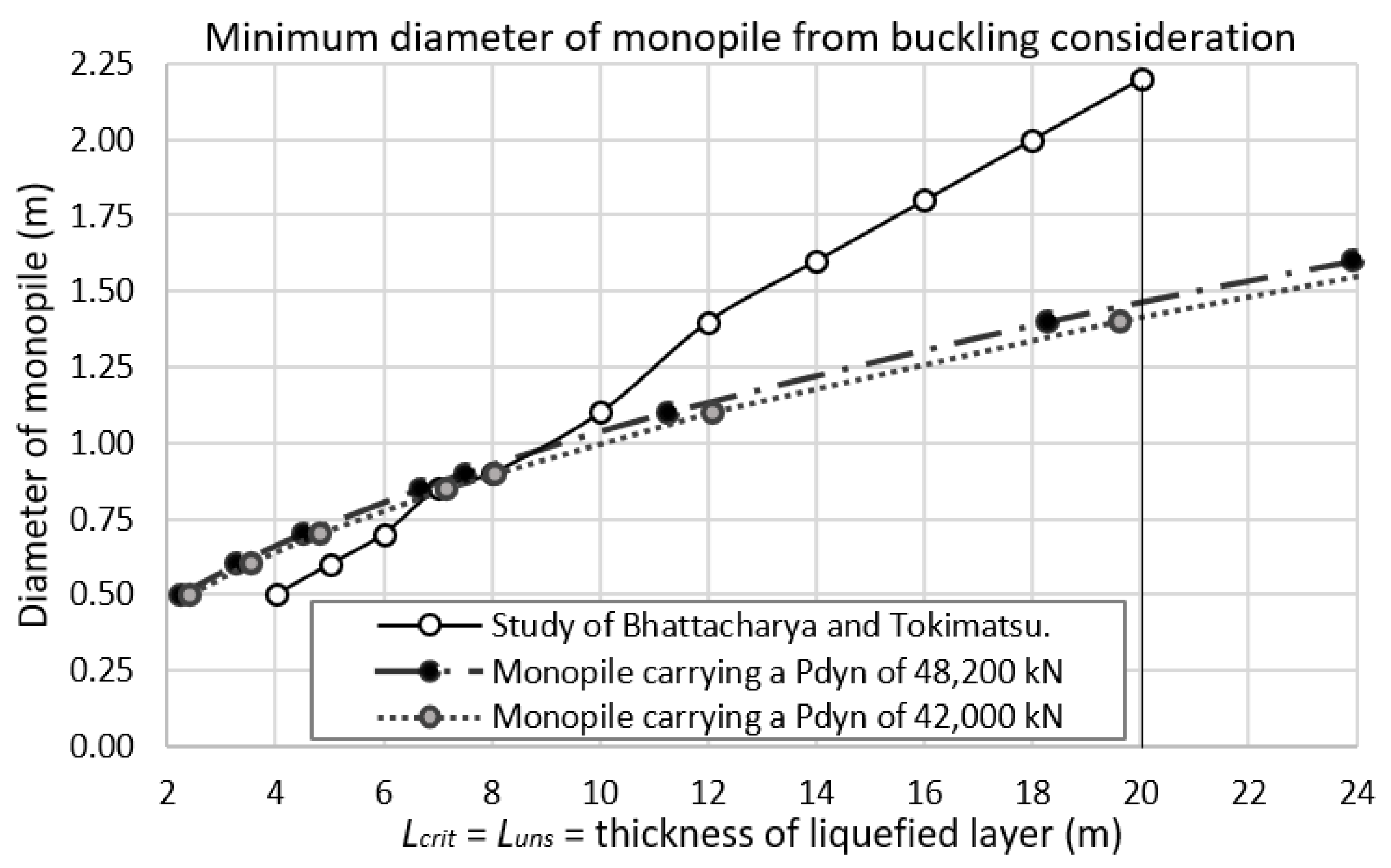
• The validation using the study of Bhattacharya and Tokimatsu [40] showed good agreement for 0.85–0.90 m monopile diameters, where the condition of L_crit = L_uns occurred at 6.69–8.05 m depths from the ground level. However, with a smaller diameter than 0.85 m, the estimated L_crit = L_uns condition was at lesser depths, while for a larger diameter than 0.90 m, the estimated L_crit = L_uns condition was at deeper depths.
• The deepest reach of liquefaction was at 20 m deep [46], in which the suggested pile diameter was 2.20 m [40]. However, the current study estimated a minimum pile diameter of 1.50 m, which was smaller by 46.6%.
• The increase in P_dyn significantly affected the large-diameter monopiles because the movement of L_crit required a longer range than the monopiles with smaller diameters.
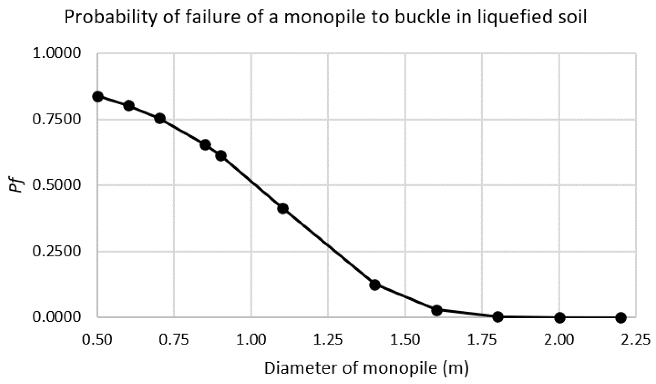
• Buckling will likely occur in monopiles with diameters of 0.5–1.60 m in fully liquefied soil because the P_f value is nearly one. On the other hand, buckling will likely not happen in monopiles with diameters of 1.80–2.20 m because the P_f value is zero. Hence, the reliable monopile diameter was 1.80 m for the current study’s HSR bridge model.
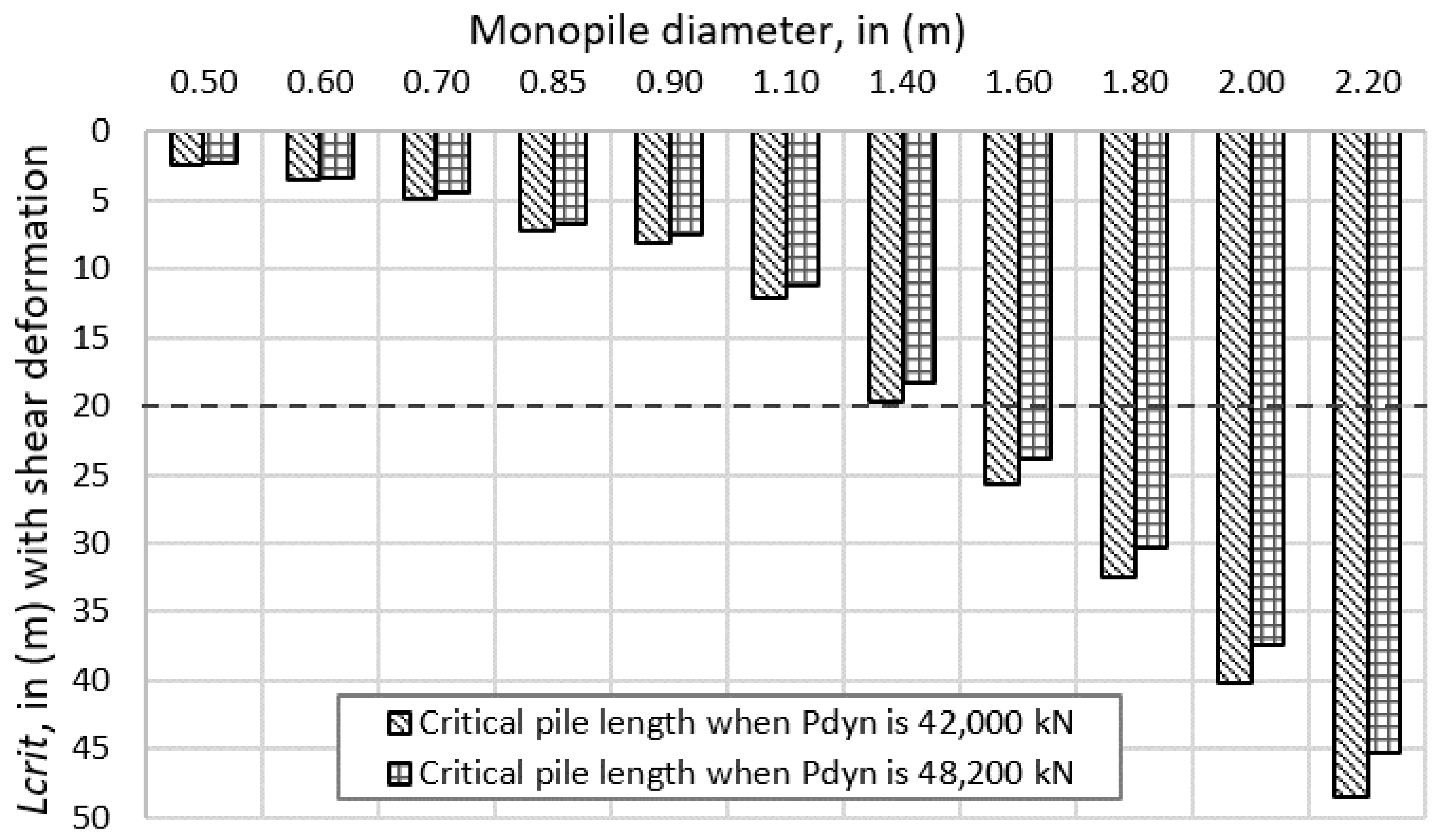
• The current study also analyzed the effect of shear deformation on large-diameter monopiles. The difference in the analysis outcome was 0.30% of L_crit, indicating that shear deformation has less of an effect on large-diameter monopile buckling.

It is important to note that the specific analysis approach depends on the site conditions, the type of structure, and the engineering requirements. In liquefied soil situations, addressing the monopile’s axial load behavior as a column element is often a more accurate representation of the monopile’s response to the ground conditions.

The feasible pile failure mechanisms are shear, bending, buckling, and cyclic loading [16]. This study focused on one failure mechanism, namely pure buckling of a monopile with the effect of shear deformation. Hence, future research shall focus on the following:

• The transformed coordinate system, illustrated in Figure 4b, by Hasofer and Lind can be further developed to visually indicate the limit state surface because it is an isosceles triangle representation. If the perpendicular distance from the longest side of the triangle to the (0,0) origin is farther, then this might indicate a lower likelihood of failure. However, if the perpendicular distance from the longest side of the triangle to the origin is too close, then this might indicate a greater likelihood of failure.
• Treating the monopile as a beam element might oversimplify the structural reliability assessment and neglect important considerations related to the monopile’s axial response. The technical reason for this is that beam element analysis typically involves studying bending moments, shear forces, and deflections, which may not be as relevant in liquefied soil conditions, where the primary concern is often the monopile’s axial capacity to support vertical loadings without buckling instability.
• The monopile may fail due to combined failure mechanisms, such as buckling, bending, and torsion, in which axial compression, lateral deformation, and rotational loading act simultaneously on the pile during the transient stage, a short period from the phase with no soil liquefaction to the fully liquefied soil phase [55].

The limitations of the current study are the following:

• The research considered a pile fixity depth (D_fix) sufficiently anchored on hard strata to secure the pile bottom while considering no settlement and overturning. The complex behavior of liquefied soil is challenging to model accurately, and it can vary depending on factors such as the soil type, density, and initial conditions.
• The HSR bridge model assumed a fully fixed rigid connection between the pier column and monopile foundation, in which the pier column remained elastic during earthquake shaking. The fixed connection means that the two elements (the bridge pier and monopile) did not rotate or move relative to each other.
• The current study did not consider the transient stage of liquefaction. During a short period from no soil liquefaction to fully liquefied soil, the monopile experiences a range of loading conditions. The dynamics of soil liquefaction may significantly impact the pile’s behavior and resistance.

References

1. Bachinilla, B.; Evangelista, A.; Siddhpura, M.; Haddad, A.N.; da Costa, B.B.F. High-Speed Railway Bridge and Pile Foundation: A Review. Infrastructures 2022, 7, 154. [Google Scholar] [CrossRef]
2. Mallick, M.; Mandal, K.K.; Sahu, R.B. A Case Study of Liquefaction-Induced Damage to a Port Building Supported on Pile Foundation. In Dynamics of Soil and Modelling of Geotechnical Problems; Satyanarayana Reddy, C.N.V., Krishna, A.M., Satyam, N., Eds.; Springer: Singapore, 2022; pp. 319–330. [Google Scholar]
3. Kramer, S.L. Geotechnical Earthquake Engineering; Prentice-Hall Civil Engineering and Engineering Mechanics Series; Prentice Hall: Upper Saddle River, NJ, USA, 1996. [Google Scholar]
4. Wang, C.-Y.; Manga, M. Liquefaction. In Water and Earthquakes; Wang, C.-Y., Manga, M., Eds.; Springer International Publishing: Cham, Switzerland, 2021; pp. 301–321. [Google Scholar]
5. Cubrinovski, M.; Ntritsos, N. 8th Ishihara lecture: Holistic evaluation of liquefaction response. Soil Dyn. Earthq. Eng. 2023, 168, 107777. [Google Scholar] [CrossRef]
6. Selcukhan, O.; Ekinci, A. Assessment of Liquefaction Hazard and Mapping Based on Standard Penetration Tests in the Long Beach and Tuzla Regions of Cyprus. Infrastructures 2023, 8, 99. [Google Scholar] [CrossRef]
7. Taftsoglou, M.; Valkaniotis, S.; Karantanellis, S.; Goula, E.; Papathanassiou, G. Preliminary Mapping of Liquefaction Phenomena Triggered by the February 6, 2023, M7.7 Earthquake, Türkiye/Syria, based on Remote Sensing. Zenodo 2023. [Google Scholar] [CrossRef]
8. Dal Zilio, L.; Ampuero, J.-P. Earthquake doublet in Turkey and Syria. Commun. Earth Environ. 2023, 4, 71. [Google Scholar] [CrossRef]
9. Liu-Zeng, J.; Wang, P.; Zhang, Z.; Li, Z.; Cao, Z.; Zhang, J.; Yuan, X.; Wang, W.; Xing, X. Liquefaction in western Sichuan Basin during the 2008 Mw 7.9 Wenchuan earthquake, China. Tectonophysics 2017, 694, 214–238. [Google Scholar] [CrossRef]
10. Zhou, X.; Lu, X.; Mou, T.; Liu, Z. Analysis of the Prevention Measures for Earthquake Damage and Flood Disasters of Bridges in Mountainous Areas of Sichuan. J. Phys. Conf. Ser. 2020, 1624, 042042. [Google Scholar] [CrossRef]
11. Finn, W.D.; Fujita, N. Piles in liquefiable soils: Seismic analysis and design issues. Soil Dyn. Earthq. Eng. 2002, 22, 731–742. [Google Scholar] [CrossRef]
12. Madabhushi, G.; Knappett, J.; Haigh, S. Design of Pile-Foundations in Liquefiable Soils; Imperial College Press: London, UK, 2010. [Google Scholar]
13. Hsu, J.T.; Aila, W.; Chang, C.H. Monopile design applied in the Panama metro line 2. In Proceedings of the 16th Asian Regional Conference on Soil Mechanics and Geotechnical Engineering, ARC 2019, Taipei, Taiwan, 14–18 October 2019; Volume 2, pp. 2–4. Available online: https://yo-1.ct.ntust.edu.tw:8887/tgssp/file/16ARC/file/YGES-003_YGES15.pdf (accessed on 13 March 2022).
14. Gauthier, Y.; Montens, S.; Paineau, T.; Arnaud, P. Dubai metro challenge for a fast track construction. In Tailor Made Concrete Structures; CRC Press—Taylor and Francis Group: Boca Raton, FL, USA, 2008; pp. 982–997. [Google Scholar]
15. Empelmann, M.; Whittaker, D.; Los, E.; Dorgarten, H.-W. Taiwan High-Speed Rail Project—Seismic Design of Bridges across the Tuntzuchiao Active Fault. In Proceedings of the 13th World Conference on Earthquake, Vancouver, BC, Canada, 1–6 August 2004; pp. 1–14. Available online: https://www.iitk.ac.in/nicee/wcee/thirteenth_conf_Canada/ (accessed on 12 August 2023).
16. Adak, G.; Bhattacharya, G.; Bhattacharya, S. Failure Mechanisms of Piles in Liquefiable Soils. In Proceedings of the 17th International Conference on Soil Mechanics and Geotechnical Engineering, Alexandria, Egypt, 5–9 October 2009; IOS Press: Amsterdam, The Netherlands, 2009; Volume 1–4, pp. 1177–1180. [Google Scholar] [CrossRef]
17. Fardis, M.; Carvalho, E.; Elnashai, A.; Faccioli, E.; Pinto, P.; Plumier, A.; Gulvanessian, H. Designers’ Guide to EN 1998-1 and 1998-5. Eurocode 8: Design Provisions for Earthquake Resistant Structures; Thomas Telford Ltd.: London, UK, 2005. [Google Scholar]
18. JRA. “Specifications for Highway Bridges, Part 5, Seismic Design”. Japanese Road Association. 2012, p. 402. Available online: https://www.road.or.jp/english/publication/index.html (accessed on 12 August 2023).
19. NEHRP. NEHRP Recommended Seismic Provisions for New Buildings and Other Structures (FEMA P-2082-1). Vol. 1 and 2. Federal Emergency Management Agency (FEMA), 25 February 2020. Available online: https://www.fema.gov/node/nehrp-recommended-seismic-provisions-new-buildings-and-other-structures (accessed on 12 August 2023).
20. Adhikari, S.; Bhattacharya, S. Dynamic Instability of Pile-Supported Structures in Liquefiable Soils during Earthquakes. Shock Vib. 2008, 15, 665–685. [Google Scholar] [CrossRef]
21. Rostami, R.; Mickovski, S.B.; Hytiris, N.; Bhattacharya, S. The Dynamic Behaviour of Pile Foundations in Seismically Liquefiable Soils: Failure Mechanisms, Analysis, Re-Qualification. In Earthquakes—From Tectonics to Buildings; Salazar, W., Ed.; IntechOpen: Rijeka, Croatia, 2021; p. 32, Chapter 8. [Google Scholar]
22. Mohanty, P.; Xu, D.; Biswal, S.; Bhattacharya, S. A shake table investigation of dynamic behavior of pile supported bridges in liquefiable soil deposits. Earthq. Eng. Eng. Vib. 2021, 20, 1–24. [Google Scholar] [CrossRef]
23. Mokhtar, A.-S.A.; Abdel-Motaal, M.A.; Wahidy, M.M. Lateral displacement and pile instability due to soil liquefaction using numerical model. Ain Shams Eng. J. 2014, 5, 1019–1032. [Google Scholar] [CrossRef]
24. Zhang, X.; Tang, L.; Ling, X.; Chan, A. Critical buckling load of pile in liquefied soil. Soil Dyn. Earthq. Eng. 2020, 135, 106197. [Google Scholar] [CrossRef]
25. Bhattacharya, S. Safety Assessment of piled Buildings in Liquefiable Soils: Mathematical Tools. In Encyclopedia of Earthquake Engineering; Beer, M., Kougioumtzoglou, I.A., Patelli, E., Au, I.S.-K., Eds.; Springer: Berlin/Heidelberg, Germany, 2014; pp. 1–16. [Google Scholar]
26. Basavana Gowda, G.M.; Dinesh, S.V.; Govindaraju, L.; Babu, R.R. Effect of Liquefaction Induced Lateral Spreading on Seismic Performance of Pile Foundations. Civ. Eng. J. 2021, 7, 58–70. [Google Scholar] [CrossRef]
27. Bhattacharya, S.; Adhikari, S.; Alexander, N.A. A simplified method for unified buckling and free vibration analysis of pile-supported structures in seismically liquefiable soils. Soil Dyn. Earthq. Eng. 2009, 29, 1220–1235. [Google Scholar] [CrossRef]
28. Fernández-Escobar, C.J.; Vega-Posada, C.A.; Garcia-Aristizábal, E.F. Lateral deformation and buckling analysis of piles including shear effects: Numerical analysis. Eng. Struct. 2023, 277, 115416. [Google Scholar] [CrossRef]
29. Han, J.; Frost, J.D. Load-Deflection response of transversely isotropic piles under lateral loads. Int. J. Numer. Anal. Methods Geomech. 2000, 24, 509–529. [Google Scholar] [CrossRef]
30. Gupta, B.K.; Basu, D. Applicability of Timoshenko, Euler–Bernoulli and rigid beam theories in analysis of laterally loaded monopiles and piles. Géotechnique 2018, 68, 772–785. [Google Scholar] [CrossRef]
31. Bechtel, A.J.; Krstic, V.; Hyde, A.; LaRegina, A. Importance of modelling shear effects for flexure of laterally loaded polymer piles. Int. J. Geotech. Eng. 2022, 16, 606–615. [Google Scholar] [CrossRef]
32. Melchers, R.; Andre, T. Structural Reliability Assessment. In Structural Reliability Analysis and Prediction, 3rd ed.; John Wiley & Sons Ltd.: Chichester, UK, 2017; pp. 31–61. [Google Scholar]
33. Verma, A.K.; Srividya, A.; Karanki, D.R. (Eds.) Structural Reliability; Springer: London, UK, 2010; pp. 267–303. [Google Scholar]
34. Guan, X.; He, J. Probabilistic Models for Reliability Analysis Using Safe-Life and Damage Tolerance Methods; Pham, H., Ed.; Springer: London, UK, 2023; pp. 965–979. [Google Scholar]
35. Djami, A.B.N.; Samon, J.B.; Ousman, B.; Nguelcheu, U.N.; Nzié, W.; Ntamack, G.E.; Kenmeugne, B. Evaluation of the Reliability of a System: Approach by Monte Carlo Simulation and Application. Open J. Appl. Sci. 2024, 14, 721–739. [Google Scholar] [CrossRef]
36. Ou, Y.; Wu, Y.; Cheng, J.; Chen, Y.; Zhao, W. Response Surface Method for Reliability Analysis Based on Iteratively-Reweighted-Least-Square Extreme Learning Machines. Electronics 2023, 12, 1741. [Google Scholar] [CrossRef]
37. Thai, H.-T.; Thai, S.; Ngo, T.; Uy, B.; Kang, W.-H.; Hicks, S.J. Reliability considerations of modern design codes for CFST columns. J. Constr. Steel Res. 2021, 177, 106482. [Google Scholar] [CrossRef]
38. Hasofer, A.M.; Lind, N.C. Exact and Invariant Second-Moment Code Format. J. Eng. Mech. Div. 1974, 100, 111–121. [Google Scholar] [CrossRef]
39. Huang, J.; Griffiths, D.V. Observations on FORM in a simple geomechanics example. Struct. Saf. 2011, 33, 115–119. [Google Scholar] [CrossRef]
40. Bhattacharya, S.; Tokimatsu, K. Essential Criteria for design of piled foundations in seismically liquefiable areas. In Proceedings National Geotechnical Conference of Japan; Japanese Geotechnical Society: Niigata, Japan, 2004; pp. 1–2. [Google Scholar]
41. Euler, L. A Method of Finding Curved Lines Enjoying the Maximum-Minimum Property, or the Solution of the Isoperimetric Problem in the Broadest Sense. Geneva, Switzerland. 1744, pp. 267–268. Available online: https://archive.org/details/methodusinvenie00eule/page/266/mode/2up (accessed on 27 August 2023).
42. Timoshenko, S.P.; Gere, J.M. Theory of Elastic Stability, 2nd ed.; McGraw-Hill Book Company, Inc.: New York City, NY, USA, 1963. [Google Scholar]
43. Dong, Y.; Feng, Z.; He, J.; Chen, H.; Jiang, G.; Yin, H. Seismic Response of a Bridge Pile Foundation during a Shaking Table Test. Shock Vib. 2019, 2019, 9726013. [Google Scholar] [CrossRef]
44. Fletcher, G.F.A. Standard Penetration Test: Its Uses and Abuses. J. Soil Mech. Found. Div. 1965, 91, 67–75. [Google Scholar] [CrossRef]
45. Seed, H.B.; Idriss, I.M. Simplified Procedure for Evaluating Soil Liquefaction Potential. J. Soil Mech. Found. Div. 1971, 97, 1249–1273. [Google Scholar] [CrossRef]
46. Iwasaki, T.; Arakawa, T.; Tokida, K.-I. Simplified procedures for assessing soil liquefaction during earthquakes. Int. J. Soil Dyn. Earthq. Eng. 1984, 3, 49–58. [Google Scholar] [CrossRef]
47. Galupino, J.; Dungca, J. Estimating Liquefaction Susceptibility Using Machine Learning Algorithms with a Case of Metro Manila, Philippines. Appl. Sci. 2023, 13, 6549. [Google Scholar] [CrossRef]
48. Sonmez, H. Modification of the liquefaction potential index and liquefaction susceptibility mapping for a liquefaction-prone area (Inegol, Turkey). Environ. Geol. 2003, 44, 862–871. [Google Scholar] [CrossRef]
49. Subedi, M.; Acharya, I.P. Liquefaction hazard assessment and ground failure probability analysis in the Kathmandu Valley of Nepal. Geoenviron. Disasters 2022, 9, 1. [Google Scholar] [CrossRef]
50. Li, D.; Juang, C.H.; Andrus, R. Liquefaction potential index: A critical assessment using probability concept. J. Geoengin. 2006, 1, 11–24. [Google Scholar] [CrossRef]
51. Chen, L.-K.; Jiang, L.-Z.; Guo, W.; Liu, W.-S.; Zeng, Z.-P.; Chen, G.-W. The seismic response of high-speed railway bridges subjected to near-fault forward directivity ground motions using a vehicle-track-bridge element. Shock Vib. 2014, 2014, 985602. [Google Scholar] [CrossRef]
52. Moayedi, H.; Kalantar, B.; Abdullahi, M.M.; Rashid, A.S.A.; Nazir, R.; Nguyen, H. Determination of Young Elasticity Modulus in Bored Piles Through the Global Strain Extensometer Sensors and Real-Time Monitoring Data. Appl. Sci. 2019, 9, 3060. [Google Scholar] [CrossRef]
53. Pal, P. Dynamic Poisson’s Ratio and Modulus of Elasticity of Pozzolana Portland Cement Concrete. Int. J. Eng. Technol. Innov. 2019, 9, 131–144. Available online: https://ojs.imeti.org/index.php/IJETI/article/view/3132 (accessed on 10 September 2023).
54. Aziz, H.Y.; Ma, J. Design and analysis of bridge foundation with different codes. J. Civ. Eng. Constr. Technol. 2011, 2, 101–118. Available online: https://api.semanticscholar.org/CorpusID:55998119 (accessed on 10 September 2023).
55. Rouholamin, M.; Lombardi, D.; Bhattacharya, S. Experimental investigation of transient bending moment of piles during seismic liquefaction. Soil Dyn. Earthq. Eng. 2022, 157, 107251. [Google Scholar] [CrossRef]
Figure 1. Bridge pier on a large-diameter monopile [1].
Infrastructures 09 00123 g001
Figure 2. Mathematical formulation framework of the current study.
Infrastructures 09 00123 g002
Figure 3. Critical pile length and unsupported pile length hypothesis.
Infrastructures 09 00123 g003
Figure 4. Shearing deformation on a column element [42].
Infrastructures 09 00123 g004
Figure 5. Hasofer-Lind Reliability Index for a linear state function [38].
Infrastructures 09 00123 g005
Figure 6. Validation of the current study using Bhattacharya and Tokimatsu’s study [40].
Infrastructures 09 00123 g006
Figure 7. Critical pile length comparison of the current study.
Infrastructures 09 00123 g007
Figure 8. Probability of failure of the current study.
Infrastructures 09 00123 g008
Figure 9. Shear deformation effect of the current study.
Infrastructures 09 00123 g009