Abstract
Inverse Distance Weighting (IDW) is a common method for spatial interpolation. Still, its accuracy decreases when there is a cluster of measurement stations or when some measuring stations are hidden behind others. This paper introduces Clusters Unifying Through Hiding Interpolation (CUTHI), a simple approach to enhance IDW accuracy. CUTHI calculates a weight for each station that considers its visibility from the interpolation point, reducing the influence of clustered or hidden stations. The method is tested in three cases: elevation data, rainfall measurements, and a mathematical function. Results demonstrate that CUTHI consistently outperforms traditional IDW, especially in areas with clustered measurement stations. CUTHI also treats the bull’s eye problem. This improved accuracy makes CUTHI a valuable tool for various applications requiring precise spatial interpolation.
1. Introduction
In many scenarios, having sparse measurements in a spatial context necessitates estimating values at intermediate locations. For instance, in meteorological applications, rain gauges dispersed across a region provide discrete rainfall data, while a comprehensive understanding of precipitation patterns requires interpolating values between these measurements. A straightforward approach to such interpolation involves assigning weights to nearby measurements, with closer observations exerting a greater influence on the estimated value at the desired point. This concept underlies the Inverse Distance Weighting (IDW) method [1], which calculates a weighted average of the measurements, wherein the weights are inversely proportional to a power of the distance between the calculation point and the measurement locations.
where v(x) is the interpolated value at point x, and vj is the value of measurement j. The weight (w) that is given to each point can be calculated as follows:
where d is the distance between the interpolated point and the measurement point, and p is the power variable that affects the weight of nearby measurements.
The IDW method is very popular [2,3,4]. However, while it offers advantages in terms of simplicity and computational efficiency, it also presents certain challenges. Primarily, the method struggles to account for clustered measurement points [5]. Consider a scenario where the interpolation point lies equidistant between two measurement stations. IDW would estimate the interpolated value as the average of these two measurements. However, if an additional station exists near one of the original stations and records a similar value (due to proximity), the weighting becomes skewed, with undue emphasis placed on the clustered measurements (Figure 1). This contradicts the principle of assigning weights based on spatial distribution. Secondly, IDW encounters difficulties when extrapolating to locations distant from existing measurements. For instance, in a temperature gradient where values decrease northward, the absence of measurements in the northernmost region leads IDW to estimate values influenced significantly by southern measurements. This occurs when the distances between southern stations and the interpolation point are considerably smaller than the distance to the nearest northern measurement (Figure 2), resulting in interpolated values that may not accurately represent the spatial trend. In this case, there are three main options: (i) Far away from the stations, we will obtain the mean values (IDW). (ii) If we see a regression, it will continue. This option is problematic, because far away, we can obtain unreasonable values. (iii) We will use the nearest measurement value.

Figure 1.
An interpolated point in blue between one red measurement point on the right that has the value of 8 and a few red measurement points on the left that all have a value of 2.

Figure 2.
The blue interpolated point is much farther than the distance between the red measurement’s points.
One way to address this problem is to use fewer measuring stations; it can be performed by determining the number of measuring stations [6,7] or by setting the search radius for stations [8,9,10]. In both ways, if we plot an interpolated map, we will obtain discontinuity when moving from one area that sees a set of stations to a nearby area that sees a different set of points.
An alternative method for reducing the search radius is to change the range of influence of the stations; this can be performed by changing the power factor in the IDW weight.
Some have completed this by determining an optimal power factor according to cross-validation or experimenting with different coefficients [11,12,13].
Another common problem of the IDW is the “bull’s eye” effect [14,15], which means that a measurement point affects only a small area in the domain, especially if there is a big difference between the measurement station data and the region mean values. Another problem is the inconsistency effect that occurs when two measurement points have the “bull’s eye” effect, and between them, the IDW gives the mean values that come from other measurement stations; although if the two measurement stations have more or less the same readings, it should give those readings also between the measurement points.
2. Materials and Methods
2.1. “Clusters Unifying Through Hiding” Interpolation (CUTHI)
When we interpolate using IDW, we use all the stations in an area; it is possible to limit the number of stations numerically, for example, to use only the nearest 10 stations, and it is possible to limit by distance, for example, to use only stations that are up to 10 km away. In any of the above methods, there is a possibility that we will use stations with values that will mislead us, both because they are behind other stations, and then the information is not the most related to the point we would like to calculate, and because some stations will be next to other stations. Then we will give them an additional weight to the weight of the first station. The method to solve this situation is to check how much a certain station is hidden from other stations, and if it is hidden to a large extent, it is given a low weight.
where is the angle between the line of the interpolated point (I) and the hiding station (H) and the line of the measurement station (M) and the hiding station (H) (see Figure 3), s is the slice power and it will be discussed later in this paper.
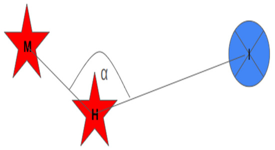
Figure 3.
Angle α when calculating the CUTHI weight is at the hiding red station (H) between the blue interpolated point (I) and the red measurement station (M).
cos (α) can take a value between minus one and one, when we add one to it, we obtain a value between zero and two, and then when we divide by two we obtain a value between zero and one. That is, when the angle is 180 degrees, meaning there is complete concealment, we will find that the station’s weight is zero, and then the station will not be used for interpolation, and when the angle is zero degrees, meaning it is located exactly behind the measurement station or behind the calculation point, it will not interfere at all and the measurement station will receive full weight since the weight function will be one. Any station that is not on a straight line connecting the calculation point to the measurement station will be subtracted from the weight given to the measurement station. When the station that can conceal is very far from the line connecting the calculation point to the measurement station, the angle that is created will be small and therefore will hardly affect the weight.
The total weight of each point will be the multiplication of the IDW weight and the clustering weight; it will replace the traditional IDW weight (Equation (2)):
In this method, stations located between the calculation point and the measurement station will hide the measurement station, and it will have less effect on the calculation point (or will not have any effect at all if the hiding station is exactly on the line connecting the calculation point and the measurement station). A cluster of stations is essentially a group of stations, some of which completely or partially hide the other stations; thus, the weight of each station in the cluster will be smaller. In the same way, when we move away from the measurement points towards the edge of the calculation area, most of the stations will appear as a cluster; therefore, for points close to the edge of the calculation area, we will effectively use only the closer stations.
2.2. Power Coefficient
The power coefficient (s) in Equation (3) governs the influence of the CUTHI weight, which ranges from 0 to 1. Maintaining this range necessitates a positive value for s. Examining two extreme scenarios illuminates its impact: When s equals zero, the CUTHI weight becomes uniformly 1, effectively rendering it inconsequential and resulting in the standard IDW function. Conversely, as s approaches a large value, the CUTHI weight exerts substantial influence, emphasizing stations that experience minimal interference from others in the calculation.
2.3. Test Cases
In this article, we will examine three test cases: The first test case is elevation data of the Mount Meron area, between latitudes 35.2 E–34.2 E and longitudes 32.2 N–32.4 N. The elevation data were taken from SRTM files with a horizontal resolution of 30 m. The average height is 443 m, the maximum height is 947, and the minimum height is −56 m. The standard deviation is 156 m.
The second test case is the mean precipitation between 1991 and 2020 in rain gauges spread around Israel. The data were taken from the Israel Meteorological Service. The average value is 506 mm, the maximum value is 988 mm, and the minimum value is 22 mm. The standard deviation is 179 mm.
The third test case is a mathematical function.
The values of x and y are between −50 and 150. This test case is purely theoretical compared to the other two test cases, which are based on experimental data. Based on 10,000 random sampling points, the average value is 27,675, the maximum value is 3,447,649, and the minimum value is −3,417,185. The standard deviation is 1,305,180.
In the test case of the mathematical function and the test case of the elevation data, there is a seemingly unlimited number of points that can be used for interpolation, each time N random points are selected. In the test case of the rain gauges, there are also hundreds of measurement stations, and N random stations are selected from them. Since we have more measurement stations than we want to display, we can choose different measurement stations in each iteration (there are iterations, when the N is high, in which some of the stations will be the same as the stations in another iteration). Using a large number of iterations for each N in each test case will strengthen the accuracy of the method.
Each of the test cases evaluates a different scenario. When we test the mathematical function, we are testing a smooth function with clear behavior. The test case of the elevations of Mount Meron is used for a function that depends on tectonic processes and natural weathering over millions of years, when the phenomenon consists of several wavelengths, a wavelength of tens of kilometers describing the mountain itself, and short wavelengths of hundreds of meters describing the wadis. The rain gauge test case shows the average annual rainfall over thirty years, and the typical distance of the rain is affected by the distance from the sea and the rain shadow desert as well as by the latitude, so the wavelengths are larger than in the previous test case. Also, averaging the data over thirty years smooths the function.
In each of the test cases, we will validate the interpolation calculation with the measurement points. We will check the correlation coefficient and the RMSD between the calculated value and the real value. The tests will compare the accuracy of IDW and the accuracy of CUTHI at different values of the power variable s.
To assess the accuracy of interpolation methods like IDW, a cross-validation approach can be employed [6,7,9]. This method involves systematically removing one measurement station at a time and using the interpolation technique to estimate the value at the removed station’s location. The estimated value is then compared to the actual measured value, allowing for the calculation of error statistics across all stations. This provides a comprehensive evaluation of the interpolation method’s performance.
For each station that is tested, we will check the mean square deviation (RMSD) and the coefficient of determination (R2). The power coefficient s in the CUTHI formula was chosen after a sensitivity test was carried out and the power in which the deviation is minimal was taken.
where N is the number of measurement stations, xk,j = 1, …, N are the measured values, and xk,i = 1, …, N are the interpolated values.
where is the mean of observed values.
3. Results
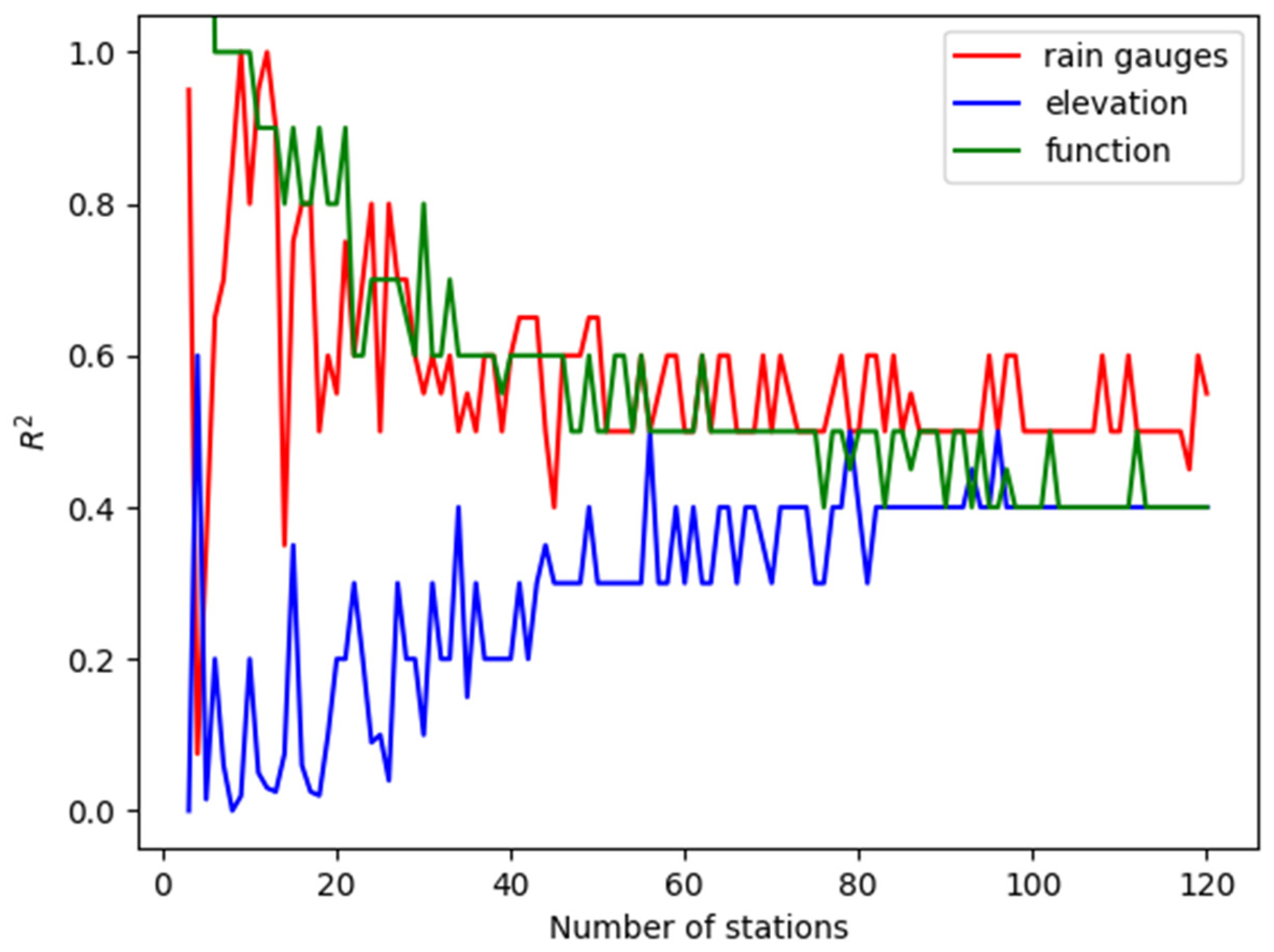
Initially, we aimed to determine the optimal coefficient s from Equation 3. To achieve this, we examined the three test cases and identified the optimal coefficient for varying numbers of measuring stations (3–120) within each case. This process was repeated 100 times for each scenario. The optimal value of s was the median value of a cross-validation for each repeat. Figure 4 presents the optimal median value of S, chosen over the mean due to its higher likelihood of representing the true optimal value. The figure illustrates the best value of s as a function of the number of stations for rain gauges (red), elevation map (blue), and the mathematical function (green). While the optimal coefficient fluctuates with a low number of stations, it generally decreases for the mathematical function and rain gauges and increases for the elevation data, ultimately converging to a similar value for a high number of stations. The variation in optimal s values across the 100 experiments, each with different station locations, suggests that the spatial arrangement of stations may also influence the ideal coefficient value.

Figure 4.
The value of s that gives the minimal error as a function of measuring points for the rain gauges test case (red), the elevation map (blue), and the mathematical function (green).
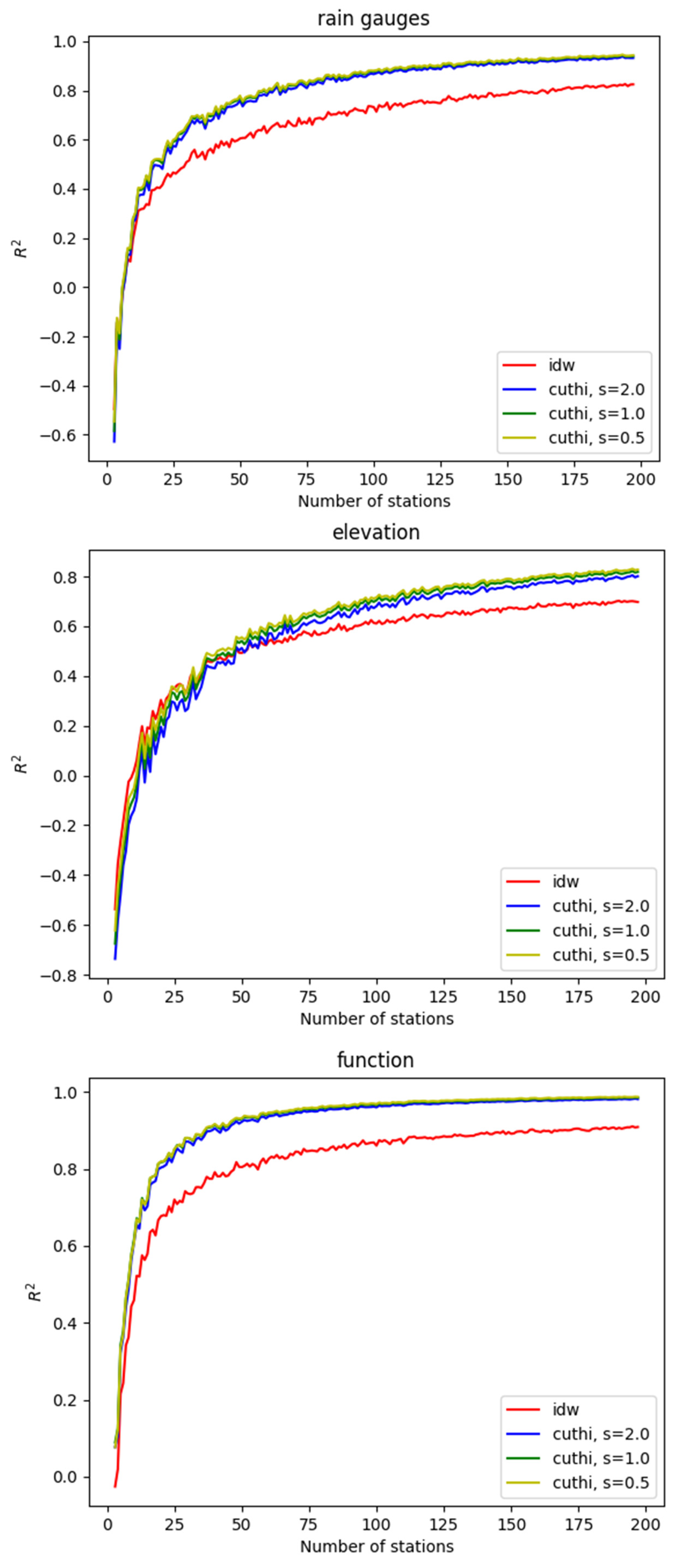
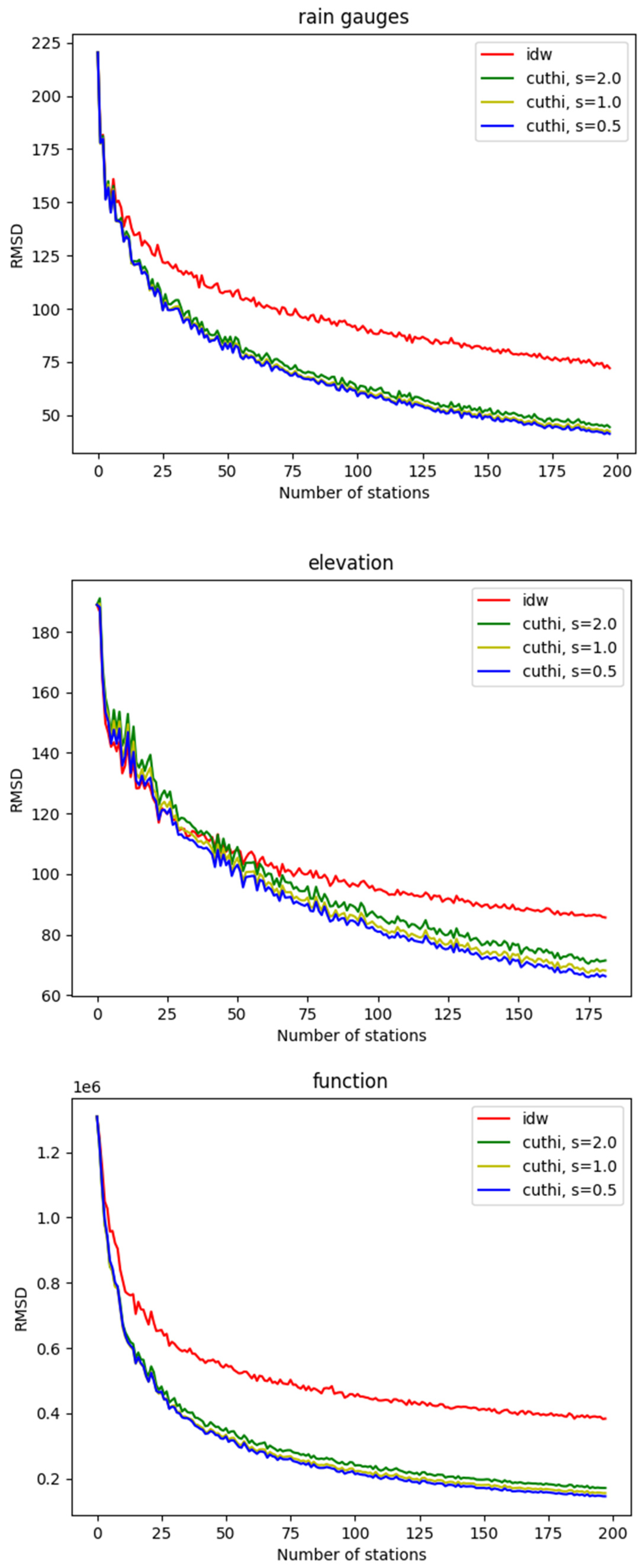
The accuracy of CUTHI was compared to IDW across various test cases. Figure 5 illustrates the coefficient of determination for the rainfall measurements (upper panel), the elevation data in the Mount Meron area (middle panel), and the mathematical function (lower panel) with the accuracy plotted as a function of the number of stations. IDW accuracy is shown in red, while CUTHI accuracy is depicted for different power values (s): blue for s = 2.0, green for s = 1.0, and yellow for s = 0.5. Figure 6 illustrates the RMSD for the same cases. One can see that CUTHI generally outperforms IDW when there are more than 10 rain gauges, 10 function points, or 25 elevation points. This suggests that CUTHI is particularly effective when sufficient stations are available to achieve good results, as indicated by a positive R2 value in cross-validation. However, this criterion may not always be necessary, especially when interpolating points are near existing stations, as cross-validation was primarily tested for stations that are not in close proximity. The clustering effect, which CUTHI aims to address, becomes more prevalent with a larger number of stations. Among the test cases, power coefficients, s = 0.5 appear to yield slightly higher accuracy.
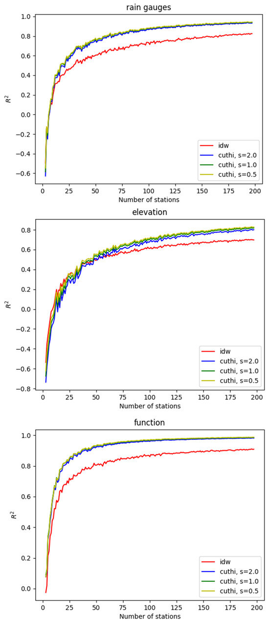
Figure 5.
The accuracy (R2) of IDW and CUTHI as a function of stations for the rain gauges test case (upper panel), elevation test case (middle panel), and function test case (lower panel).
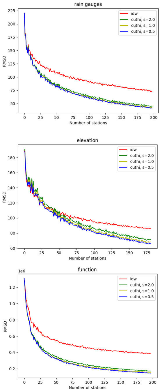
Figure 6.
The same as Figure 5 but for RMSD.
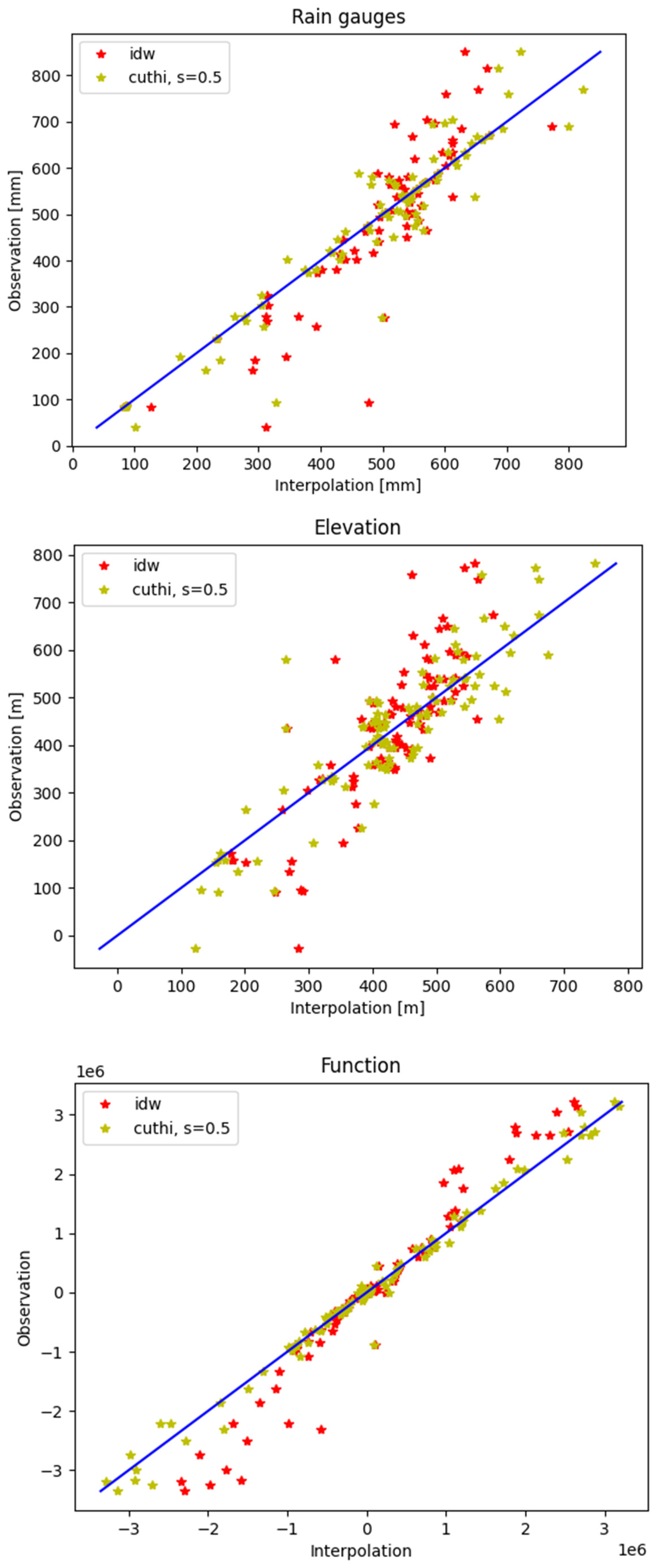
Figure 7 shows the correlation between the measurements and the interpolation calculations in one iteration for the three test cases. The RMSD of the rain gauges (upper panel) is 80 mm when using IDW and 55 mm when using CUTHI. The RMSD of the elevation data (middle panel) is 95 m when using IDW and 72 m when using CUTHI. And the RMSD of the function (lower panel) is 468,926 when using IDW and 171,431 when using CUTHI.
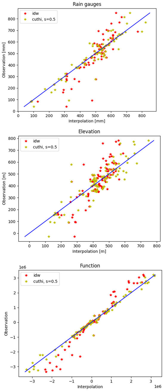
Figure 7.
The correlation between the observation data and the interpolation data for IDW (red) and CUTHI (yellow) for the rain gauges test case (upper panel), elevation test case (middle panel), and function test case (lower panel). The blue line represents a perfect match.
It can be seen that in the middle of the graph, at the mean values, the accuracy of both IDW and CUTHI is high, but as we move away from those values, CUTHI shows higher accuracy. It can be seen that at low values, the IDW shows higher values that are closer to the mean values and at high values, the IDW shows lower values that are also closer to the mean values. This behavior is observed in all three cases.
To generate an interpolated map, values are calculated at each point based on the desired resolution. Figure 8 depicts a rainfall map generated using both IDW (right panel) and CUTHI (left panel) interpolation methods, based on data from rain gauges. While both methods display measured values at their corresponding locations, differences become apparent between stations and beyond the calculation area. Notably, IDW tends towards the average value of all stations as the distance from measurement points increases, even within the interpolation area. In contrast, CUTHI’s calculated values are primarily influenced by the nearest stations. This effect is particularly pronounced at the boundaries of the calculation area. Additionally, “bull’s-eye” patterns observed in IDW (e.g., in the lower left corner) are absent in the CUTHI interpolation.
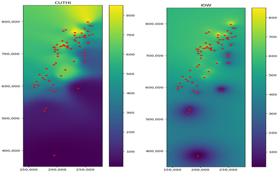
Figure 8.
Interpolation maps of the rain gauges test case using IDW (right panel) and CUTHI (left panel).
4. Discussion and Conclusions
This work presents CUTHI, a novel interpolation method that builds upon the strengths of IDW while addressing its key limitations. By accounting for the spatial arrangement of measurement points and mitigating the influence of clustered or hidden stations, CUTHI consistently outperforms traditional IDW in terms of accuracy, particularly in regions with clustered data. The method’s effectiveness has been demonstrated across diverse test cases, including elevation data, rainfall measurements, and a mathematical function.
If the space in which we want to perform interpolation has many measurement stations, we would want to use only the stations that help us find the value at the required location and would like to avoid using stations that interfere with our ability to calculate the value at the required location. CUTHI’s method of classifying the stations into stations that help and stations that interfere, or essentially giving a score for how helpful the station is by using a hiding function. The hiding function is determined by the angle between the calculation point, the hiding station, and the station that influences the calculation. So, if the concealment station is exactly on the path between the calculation point and the measurement station, the concealment will be maximum; if the concealment station is exactly behind the measurement station with respect to the calculation point or behind the calculation point with respect to the measurement station, there will be no concealment at all. In this way, when we have a cluster of stations, each station will give some of the information and the ratio to the cluster will be approximately the same as for one station. We wrote approximately, because this station is actually of a larger effective size.
CUTHI’s ability to overcome the “bull’s eye” and inconsistency effects commonly associated with IDW further underscores its advantages. Moreover, its simplicity makes it a valuable tool for a wide range of applications that demand precise spatial interpolation. The adaptability of CUTHI to higher dimensions expands its potential utility in various scientific and engineering domains.
While CUTHI represents a significant advancement in spatial interpolation, future research could explore further refinements and extensions. Investigating the relationship between the optimal power coefficient and the spatial distribution of measurement points could lead to more tailored and adaptive implementations. Additionally, exploring the integration of CUTHI with other interpolation techniques (e.g., Kriging) or data fusion approaches could unlock new possibilities for enhanced accuracy and robustness in complex spatial analysis tasks.
In conclusion, CUTHI offers a compelling solution to the challenges posed by clustered measurement points in spatial interpolation. Its superior accuracy and simplicity position it as a valuable asset for researchers and practitioners across various fields. As spatial data continue to proliferate, CUTHI’s ability to extract meaningful insights from such data will undoubtedly contribute to advancements in diverse areas of study and application.
Funding
This research received no external funding.
Informed Consent Statement
Not applicable.
Data Availability Statement
An example code can be found at https://github.com/bambiker/interpolation (accessed on 4 March 2025).
Acknowledgments
The author would like to thank Noam Halfom from IMS for providing the rain gauges data.
Conflicts of Interest
The author declares no conflicts of interest.
References
- Shepard, D. A two-dimensional interpolation function for irregularly-spaced data. In Proceedings of the 1968 23rd ACM National Conference, Las Vegas, NV, USA, 27–29 August 1968; ACM: New York, NY, USA, 1968; pp. 517–524. [Google Scholar]
- Xie, P.; Arkin, P.A. Global precipitation: A 17-year monthly analysis based on gauge observations, satellite estimates, and numerical model outputs. Bull. Am. Meteorol. Soc. 1997, 78, 2539–2558. [Google Scholar] [CrossRef]
- Kishore, P.; Jyothi, S.; Basha, G.; Rao, S.V.B.; Rajeevan, M.; Velicogna, I.; Sutterley, T.C. Precipitation climatology over India: Validation with observations and reanalysis datasets and spatial trends. Clim. Dyn. 2016, 46, 541–556. [Google Scholar] [CrossRef]
- Basha, G.; Kishore, P.; Ratnam, M.V.; Jayaraman, A.; Agha Kouchak, A.; Ouarda, T.B.; Velicogna, I. Historical and Projected Surface Temperature over India during the 20th and 21st century. Sci. Rep. 2017, 7, 2987. [Google Scholar] [CrossRef] [PubMed]
- Li, Z.; Wang, K.; Ma, H.; Wu, Y. An adjusted inverse distance weighted spatial interpolation method. In Proceedings of the 2018 3rd International Conference on Communications, Information Management and Network Security (CIMNS 2018), Wuhan, China, 27–28 November 2018; pp. 128–132. [Google Scholar]
- Chen, F.W.; Liu, C.W. Estimation of the spatial rainfall distribution using inverse distance weighting (IDW) in the middle of Taiwan. Paddy Water Environ. 2012, 10, 209–222. [Google Scholar] [CrossRef]
- Li, L.; Losser, T.; Yorke, C.; Piltner, R. Fast inverse distance weighting-based spatiotemporal interpolation: A web-based application of interpolating daily fine particulate matter PM2.5 in the contiguous US using parallel programming and kd tree. Int. J. Environ. Res. Public Health 2014, 11, 9101–9141. [Google Scholar] [CrossRef] [PubMed]
- Tanır Kayıkçı, E.; Zengin Kazancı, S. Comparison of regression-based and combined versions of inverse distance weighted methods for spatial interpolation of daily mean temperature data. Arab. J. Geosci. 2016, 9, 690. [Google Scholar] [CrossRef]
- Malvić, T.; Ivšinović, J.; Velić, J.; Sremac, J.; Barudžija, U. Application of the Modified Shepard’s Method (MSM): A Case Study with the Interpolation of Neogene Reservoir Variables in Northern Croatia. Stats 2020, 3, 68–83. [Google Scholar] [CrossRef]
- Liu, Z.N.; Yu, X.Y.; Jia, L.F.; Wang, Y.S.; Song, Y.C.; Meng, H.D. The influence of distance weight on the inverse distance weighted method for ore-grade estimation. Sci. Rep. 2021, 11, 2689. [Google Scholar] [CrossRef] [PubMed]
- Lu, G.Y.; Wong, D.W. An adaptive inverse-distance weighting spatial interpolation technique. Comput. Geosci. 2008, 34, 1044–1055. [Google Scholar] [CrossRef]
- Liu, Z.; Zhang, Z.; Zhou, C.; Ming, W.; Du, Z. An Adaptive Inverse-Distance Weighting Interpolation Method Considering Spatial Differentiation in 3D Geological Modeling. Geosciences 2021, 11, 51. [Google Scholar] [CrossRef]
- Choi, K.; Chong, K. Modified Inverse Distance Weighting Interpolation for Particulate Matter Estimation and Mapping. Atmosphere 2022, 13, 846. [Google Scholar] [CrossRef]
- Ren, X.; Cabaravdic, M.; Zhang, X.; Kuhlenkotter, B. A local process model for simulation of robotic belt grinding. Int. J. Mach. Tools Manuf. 2007, 47, 962–970. [Google Scholar] [CrossRef]
- Shi, W.; Liu, J.; Du, Z.; Song, Y.; Chen, C.; Yue, T. Surface modelling of soil pH. Geoderma 2009, 150, 113–119. [Google Scholar] [CrossRef]


Disclaimer/Publisher’s Note: The statements, opinions and data contained in all publications are solely those of the individual author(s) and contributor(s) and not of MDPI and/or the editor(s). MDPI and/or the editor(s) disclaim responsibility for any injury to people or property resulting from any ideas, methods, instructions or products referred to in the content. |
© 2025 by the author. Licensee MDPI, Basel, Switzerland. This article is an open access article distributed under the terms and conditions of the Creative Commons Attribution (CC BY) license (https://creativecommons.org/licenses/by/4.0/).